Chiral extrapolation beyond the power-counting regime

Abstract

Chiral effective field theory can provide valuable insight into the chiral physics of hadrons when used in conjunction with non-perturbative schemes such as lattice quantum chromodynamics (QCD). In this discourse, the attention is focused on extrapolating the mass of the $\rho$ meson to the physical pion mass in quenched QCD (QQCD). With the absence of a known experimental value, this serves to demonstrate the ability of the extrapolation scheme to make predictions without prior bias. By using extended effective field theory developed previously, an extrapolation is performed using quenched lattice QCD data that extends outside the chiral power-counting regime (PCR). The method involves an analysis of the renormalization flow curves of the low-energy coefficients in a finite-range regularized effective field theory. The analysis identifies an optimal regularization scale, which is embedded in the lattice QCD data themselves. This optimal scale is the value of the regularization scale at which the renormalization of the low-energy coefficients is approximately independent of the range of quark masses considered. By using recent precision, quenched lattice results, the extrapolation is tested directly by truncating the analysis to a set of points above $380$ MeV, while temporarily disregarding the simulation results closer to the chiral regime. This tests the ability of the method to make predictions of the simulation results, without phenomenologically motivated bias. The result is a successful extrapolation to the chiral regime.

I Introduction

In lattice quantum chromodynamics (QCD), the calculation of observables with light dynamical quarks is computationally intensive, and only in recent times have there been successful attempts to perform calculations of any observable at the physical point ($m_{\pi}=140$ MeV) Aoki et al. (2009); Kuramashi (2008); Durr et al. (2010). Usually, some extrapolation scheme is needed if one is to compare theoretical calculations with the corresponding physical observables. Utilizing lattice QCD results spread over a larger range of quark masses naturally enables greater statistical precision in the extrapolation.

Quenched QCD (QQCD) was introduced as a way to ameliorate the computational difficulty of simulating dynamical fermions on the lattice. Quenched simulations typically have been superseded by the wide availability of dynamical configurations. Nevertheless, it can still be used as an efficient testing ground. This is particularly true of the chiral extrapolation problem, where the experimentally known values may introduce a prejudice on a chosen form. In QQCD, the physical target point does not exist, and an extrapolation of moderate-mass points to the chiral regime provides an unbiased test of the procedure.

In order to discuss the chiral behaviour of the $\rho$ meson in QQCD, one first constructs an effective field theory describing the relevant low-energy degrees of freedom. The mass of the $\rho$ meson is described by a chiral expansion in the quark mass ($m_{q}$), which includes analytic terms that are polynomial in $m_{q}$, and non-analytic terms arising from chiral loop integrals. These loop integrals are commonly divergent, and thus it is necessary to introduce a regularization procedure. Finite-range regularization (FRR) is selected as a regularization scheme, which introduces a momentum cutoff scale $\Lambda$ into the loop integrals. The properties of FRR allow it to be used with data extending outside the power-counting regime (PCR), at the expense of complete scheme-independence. As has been demonstrated, an optimal choice of regularization scale, $\Lambda_{\mathrm{scale}}$, can be extracted from the lattice simulation results Hall et al. (2010). A systematic uncertainty in $\Lambda_{\mathrm{scale}}$ can also be estimated, which provides a range of suitable values for the scale obtained from the data Young et al. (2009). Thus the scheme-dependence in using data extending outside the PCR can be quantified in an unbiased fashion.

II Extended effective field theory

In chiral effective field theory ($\chi$EFT), the diagrammatic formulation can be used to identify the major contributions to the $\rho$ meson mass in QQCD Chow and Rey (1998); Armour et al. (2006). The leading-order diagrams are the double and single $\eta^{\prime}$ hairpin diagrams as shown in Figures 2 and 2, respectively. The constant coefficients of these loop integrals are endowed with an uncertainty to encompass the possible effects of smaller contributions to order $\mathcal{O}(m_{\pi}^{4})$.

Figure 1: Double hairpin $\eta^{\prime}$ diagram.

Figure 2: Single hairpin $\eta^{\prime}$ diagram.

Interactions with the flavour-singlet $\eta^{\prime}$ are the most important contributions to the $\rho$ meson mass in QQCD. This is an artifact of the quenched approximation, where the $\eta^{\prime}$ also behaves as a pseudo-Goldstone boson, having a “mass” that is degenerate with the pion. The dressing of the $\rho$ meson by the $\eta^{\prime}$ field is illustrated in Figures 5 through 5. Since the hairpin vertex must be a flavor-singlet, the mesons that can contribute are the $\eta^{\prime}$ meson, and the $\omega$ meson. The contributions from the $\omega$ meson are insignificant due to OZI suppression and the small $\rho$-$\omega$ mass splitting. However, in QQCD, the $\eta^{\prime}$ loop behaves much as a pion loop, yet with a slightly modified propagator.

Figure 3: Double hairpin quark flow diagram.

Figure 4: Alternative double hairpin quark flow diagram.

Figure 5: Single hairpin quark flow diagram.

In full QCD however, the $\eta^{\prime}$ does not play any role in the low-energy dynamics. The physical $\eta^{\prime}$ acquires a finite mass — which survives in the chiral limit — by re-summing the chain of vacuum insertions as depicted in Figure 6.

Figure 6: Diagrammatic representation of $\eta^{\prime}$ propagator terms.

As a “heavy” degree of freedom, the $\eta^{\prime}$ can then be integrated out of the of the effective field theory.

II.1 Loop integrals and definitions

Using the Gell-Mann$-$Oakes$-$Renner Relation connecting quark and pion masses (assuming negligible anomalous scaling), $m_{q}\propto m_{\pi}^{2}$ Gell-Mann et al. (1968), the $\rho$ meson mass extrapolation formula in QQCD can be expressed in a form that contains an analytic polynomial in $m_{\pi}^{2}$ plus the chiral loop integrals ($\Sigma^{Q}$):

$$m_{\rho,Q}^{2} =a_{0}+a_{2}m_{\pi}^{2}+a_{4}m_{\pi}^{4}$$

$$+\Sigma_{\eta^{\prime}\!\eta^{\prime}}^{Q}(m_{\pi}^{2},\Lambda)+\Sigma_{\eta^{\prime}}^{Q}(m_{\pi}^{2},\Lambda)+\mathcal{O}(m_{\pi}^{5}).$$ (1)

The coefficients $a_{i}$ are the ‘residual series’ coefficients, which correspond to direct quark-mass insertions in the underlying Lagrangian of chiral perturbation theory. However, the non-analytic behaviour of the expansion arises from the chiral loop integrals. Upon renormalization of the divergent loop integrals, these will correspond with low-energy constants of the quenched $\chi$EFT. The extraction of these parameters from lattice QCD results will now be demonstrated.

By convention, the non-analytic terms from the double and single hairpin integrals are $\chi_{1}m_{\pi}$ and $\chi_{3}m_{\pi}^{3}$, respectively. The coefficients $\chi_{1}$ and $\chi_{3}$ of the leading-order non-analytic terms are scheme-independent constants that can be estimated from phenomenology. The low-order expansion of the loop contributions takes the following form:

$$\Sigma_{\eta^{\prime}\!\eta^{\prime}}^{Q} =b^{\eta^{\prime}\!\eta^{\prime}}_{0}+\chi_{1}m_{\pi}+b^{\eta^{\prime}\!\eta^{\prime}}_{2}m_{\pi}^{2}+\chi_{3}^{\eta^{\prime}\!\eta^{\prime}}m_{\pi}^{3}+b^{\eta^{\prime}\!\eta^{\prime}}_{4}m_{\pi}^{4}$$

$$+\mathcal{O}(m_{\pi}^{6}),$$ (2)

$$\Sigma_{\eta^{\prime}}^{Q} =b^{\eta^{\prime}}_{0}+b^{\eta^{\prime}}_{2}m_{\pi}^{2}+\chi_{3}^{\eta^{\prime}}m_{\pi}^{3}+b^{\eta^{\prime}}_{4}m_{\pi}^{4}+\mathcal{O}(m_{\pi}^{6}),$$ (3)

The coefficient $\chi_{3}$ is obtained by adding the contributions from both integrals, $\chi_{3}=\chi_{3}^{\eta^{\prime}\!\eta^{\prime}}+\chi_{3}^{\eta^{\prime}}$. Each integral has a solution in the form of a polynomial expansion analytic in $m_{\pi}^{2}$ plus non-analytic terms, of which the leading-order term is of greatest interest. The coefficients $b_{i}$ are scale-dependent and therefore scheme-dependent. In order to achieve an extrapolation based on an optimal FRR scale, first the scale-dependence of the low-energy expansion must be removed through renormalization. The renormalization program of FRR combines the scheme-dependent $b_{i}$ coefficients from the chiral loops with the scheme-dependent $a_{i}$ coefficients from the residual series at each chiral order $i$. The result is a scheme-independent coefficient $c_{i}$:

$$c_{0} =a_{0}+b_{0}^{\eta^{\prime}\!\eta^{\prime}}+b_{0}^{\eta^{\prime}},$$ (4)

$$c_{2} =a_{2}+b_{2}^{\eta^{\prime}\!\eta^{\prime}}+b_{2}^{\eta^{\prime}},$$ (5)

$$c_{4} =a_{4}+b_{4}^{\eta^{\prime}\!\eta^{\prime}}+b_{4}^{\eta^{\prime}},\mbox{\,\,etc.}$$ (6)

That is, the underlying $a_{i}$ coefficients undergo a renormalization from the chiral loop integrals. The renormalized coefficients $c_{i}$ are an important part of the extrapolation technique. A stable and robust determination of these parameters forms the core of determining an optimal scale $\Lambda^{\mathrm{scale}}$.

The loop integrals can be expressed in a convenient form by taking the non-relativistic limit and performing the pole integration for $k_{0}$. Renormalization is achieved by subtracting the relevant terms in the Taylor expansion of the loop integrals and absorbing them into the corresponding low-energy coefficients, $c_{i}$:

$$\tilde{\Sigma}_{\eta^{\prime}\!\eta^{\prime}}^{Q}(m_{\pi}^{2};\Lambda) =\frac{-\chi_{\eta^{\prime}\!\eta^{\prime}}}{3\pi^{2}}\int\!\!\mathrm{d}^{3}k\frac{(M_{0}^{2}k^{2}+\frac{5}{2}A_{0}k^{4})u^{2}(k;\Lambda)}{{(k^{2}+m_{\pi}^{2})}^{2}}$$

$$-b_{0}^{\eta^{\prime}\!\eta^{\prime}}-b_{2}^{\eta^{\prime}\!\eta^{\prime}}m_{\pi}^{2}-b_{4}^{\eta^{\prime}\!\eta^{\prime}}m_{\pi}^{4},$$ (7)

$$\tilde{\Sigma}_{\eta^{\prime}}^{Q}(m_{\pi}^{2};\Lambda) =\frac{\chi_{\eta^{\prime}}}{2\pi^{2}}\int\!\!\mathrm{d}^{3}k\frac{k^{2}u^{2}(k;\Lambda)}{k^{2}+m_{\pi}^{2}}-b_{0}^{\eta^{\prime}}-b_{2}^{\eta^{\prime}}m_{\pi}^{2}$$

$$-b_{4}^{\eta^{\prime}}m_{\pi}^{4}.$$ (8)

The tilde ($\,\tilde{\,}\,$) denotes that the integrals are written out in renormalized form to chiral order $\mathcal{O}(m_{\pi}^{4})$. The coefficients $\chi_{\eta^{\prime}\!\eta^{\prime}}$ and $\chi_{\eta^{\prime}}$ are related to the coefficients of the leading-order non-analytic terms by:

$$\chi_{1} =M_{0}^{2}\,\chi_{\eta^{\prime}\!\eta^{\prime}},$$ (9)

$$\chi_{3} =\chi_{3}^{\eta^{\prime}\!\eta^{\prime}}+\chi_{3}^{\eta^{\prime}}=A_{0}\,\chi_{\eta^{\prime}\!\eta^{\prime}}+\chi_{\eta^{\prime}}.$$ (10)

These couplings are discussed in detail below. The function $u(k;\Lambda)$ is a finite-range regulator with cutoff scale $\Lambda$, which must be normalized to $1$ at $k^{2}=0$, and must approach $0$ sufficiently fast to ensure convergence of the loop. Different functional forms of $u(k;\Lambda)$ are equivalent within the PCR Young et al. (2003); Leinweber et al. (2005). Different choices of $u(k;\Lambda)$ for this investigation are discussed in Sec. II.2.

With the loop integrals specified, Eq. (1) can be rewritten in terms of the renormalized coefficients $c_{i}$:

$$m_{\rho,Q}^{2} =c_{0}+c_{2}m_{\pi}^{2}+c_{4}m_{\pi}^{4}+\tilde{\Sigma}_{\eta^{\prime}\!\eta^{\prime}}^{Q}(m_{\pi}^{2};\Lambda)$$

$$+\tilde{\Sigma}_{\!\eta^{\prime}}^{Q}(m_{\pi}^{2};\Lambda)+\mathcal{O}(m_{\pi}^{5})$$ (11)

$$\approx c_{0}+\chi_{1}m_{\pi}+c_{2}m_{\pi}^{2}+\chi_{3}m_{\pi}^{3}+c_{4}m_{\pi}^{4}$$

$$+\mathcal{O}(m_{\pi}^{5}).$$ (12)

Eq. (II.1) will be used as the extrapolation formula for $m_{\rho,Q}$ at infinite lattice volume. The fit coefficients are $c_{0}$, $c_{2}$ and $c_{4}$, and $m_{\rho,Q}$ is obtained by taking the square root of Eqs.(II.1) and (12). It is important to note that the formula in Eq. (12) is equivalent to Eq. (II.1) only as $\Lambda$ is taken to infinity.

Since lattice simulations are necessarily carried out on a discrete spacetime, any extrapolations performed should take into account finite-volume effects. The low-energy effective field theory is ideally suited for characterising the leading infrared effects associated with the finite volume. In order to achieve this, each of the three-dimensional integrals can be transformed to its form on the lattice using a finite sum of discretized momenta, following Armour et al. Armour et al. (2006), for instance:

$$\int\!\!\mathrm{d}^{3}k\rightarrow\frac{{(2\pi)}^{3}}{L_{x}L_{y}L_{z}}\sum_{k_{x},k_{y},k_{z}}.$$ (13)

Each momentum component is quantized in units of $2\pi/L$, that is $k_{i}=n_{i}2\pi/L$ for integers $n_{i}$. Finite-volume corrections $\delta^{\mathrm{FVC}}$ can be written simply as the difference between the finite sum and the corresponding integral. It is known that the finite-volume corrections saturate to a fixed result for large values of the regularization scale Hall et al. (2010). Following the example set by this article, the value $\Lambda^{\prime}=2.0$ GeV is chosen to evaluate all finite-volume corrections independent of the FRR cutoff scale $\Lambda$ in Eqs.(II.1) and (II.1). The finite-volume version of Eq. (II.1) can thus be expressed:

$$m_{\rho,Q}^{2} =c_{0}+c_{2}m_{\pi}^{2}+c_{4}m_{\pi}^{4}+(\tilde{\Sigma}_{\eta^{\prime}\!\eta^{\prime}}^{Q}(m_{\pi}^{2};\Lambda)$$

$$+\delta^{\mathrm{FVC}}_{\eta^{\prime}\!\eta^{\prime}}(m_{\pi}^{2};\Lambda^{\prime}))+(\tilde{\Sigma}_{\!\eta^{\prime}}^{Q}(m_{\pi}^{2};\Lambda)+\delta^{\mathrm{FVC}}_{\eta^{\prime}}(m_{\pi}^{2};\Lambda^{\prime}))$$

$$+\mathcal{O}(m_{\pi}^{5}).$$ (14)

The convention used for defining the values of $\chi_{1}$, $\chi_{3}$, and the various coupling constants that occur in each, follows Booth Booth et al. (1997). For the possible different values that coupling constants can take, definitions by Chow & Rey Chow and Rey (1998), Armour et al. Armour et al. (2006) and Sharpe Sharpe (1997) are used. The types of vertices available are shown in Figure 7, where $g_{2}$ and $g_{4}$ occur explicitly in the two diagrams considered here. Booth suggests naturalness for $g_{2}\sim 1$, and that $g_{4}\sim 1/N_{c}$. These quenched coupling constants can be connected with the experimental value of $g_{\omega\rho\pi}$ as per Lublinsky Lublinsky (1997) by the relation:

$$g_{2}=\frac{1}{2}g_{\omega\rho\pi}f_{\pi},$$ (15)

where $g_{\omega\rho\pi}=14\pm 2$ GeV^-1 and the pion decay constant takes the value $f_{\pi}=0.0924$ GeV. Thus $g_{2}$ is chosen to be $0.65\pm 0.09$ GeV and $g_{4}$ is chosen to be approximately $g_{2}/3$. The coupling between the separate legs of the double hairpin diagram are approximated by the massive constant $M_{0}^{2}\propto m_{\eta^{\prime}}^{2}$. The next-order correction to $M_{0}$ in momentum $k$ defines the coupling to be $-M_{0}^{2}+A_{0}k^{2}$. These constants can be connected to the full QCD $\eta^{\prime}$ meson mass $m_{\eta^{\prime}}$ by considering the geometric series of terms as previously illustrated in Figure 6. For the value of $M_{0}$, Booth suggest $M_{0}\approx 400$ MeV by comparing the estimate from a hairpin insertion to the result from the Witten-Veneziano formula Booth et al. (1997). In a paper by Duncan et al. a value of $M_{0}\approx 900$ MeV is obtained if the coupling constant $A_{0}$ is natural. Furthermore, an analysis of the topological susceptibility leads to an estimate $M_{0}=1.1\pm 0.2$ GeV Duncan et al. (1997). In this analysis, an average value $M_{0}=(400+900+1100)/3=800$ MeV is sensible as a first approximation. As a further check, consider the formula from Ref. Duncan et al. (1997), using our normalization for the pion decay constant ($f_{\pi}^{2}=2f_{\pi,\mathrm{Duncan}}^{2}$):

$$\delta=\frac{A_{0}M_{0}^{2}}{48\pi^{2}f_{\pi}^{2}}.$$ (16)

This formula relates the couplings $A_{0}$ and $M_{0}^{2}$ to the anomalous scaling parameter of the pion mass in quenched QCD, defined by:

$$m_{\pi}^{2}\approx m_{q}^{\frac{1}{1+\delta}}.$$ (17)

The parameter $\delta$ is found to be small (and the Gell-Mann$-$Oakes$-$Renner Relation a good approximation), with a maximum value estimated by Duncan to be $\delta_{\mathrm{max}}=0.03$ Duncan et al. (1997). Booth comments that the parameter $A_{0}$ is small, and vanishes in the limit $N_{c}\rightarrow\infty$. Nevertheless, Sharpe uses a finite value $A_{0}\sim 0.2$ Sharpe (1997). By using these finite values for $\delta$ and $A_{0}$, Eq. (16) leads to a value of $M_{0}^{2}\approx 0.6$ GeV². As a result, $M_{0}^{2}$ is taken to be $0.6\pm 0.2$ GeV² and $A_{0}$ is taken to be $0\pm 0.2$.

The coefficients $\chi_{\eta^{\prime}\!\eta^{\prime}}$ and $\chi_{\eta^{\prime}}$ can be specified in terms of the relevant coupling constants:

$$\chi_{\eta^{\prime}\!\eta^{\prime}} =-2\stackrel{{\scriptstyle\circ}}{{m}}_{\rho}\!\frac{g_{2}^{2}}{4\pi f_{\pi}^{2}},$$

$$\chi_{\eta^{\prime}} =-2\stackrel{{\scriptstyle\circ}}{{m}}_{\rho}\!\frac{g_{2}g_{4}}{6\pi f_{\pi}^{2}},$$ (18)

where the couplings are defined relative to $\stackrel{{\scriptstyle\circ}}{{m}}_{\rho}$ representing the $\rho$ meson mass in the chiral limit, which is taken to be $770$ MeV.

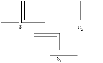
Figure 7: Coupling types following convention introduced by Booth Booth et al. (1997).

II.2 Finite-range regularization

In FRR, regulator functions $u(k;\Lambda)$ with characteristic scale $\Lambda$ are inserted into the loop integrals to control the ultraviolet divergences that occur in the loop integrals encountered. For some choices of regulator, extra regulator-dependent non-analytic terms arise in the chiral expansion of Eq. (12). Since the correct non-analytic terms of the chiral expansion are regularization scale-independent terms, the extra non-analytic terms within working chiral order must be removed. All scale-dependence should be absorbed into the analytic fit parameters $a_{i}$. For example, if a dipole regulator is chosen, the extra terms $b_{3}^{(1)}m_{\pi}^{3}$, $(b_{5}^{(1)}+b_{5}^{(3)})m_{\pi}^{5}$ and higher-order terms occurring at odd powers of $m_{\pi}$ feature in Eq. (12). One can avoid this by choosing a regulator that does not generate these extra terms, up to working-order $\mathcal{O}(m_{\pi}^{4})$. Since the step function $u^{2}(k;\Lambda)=\theta(\Lambda-k)$ introduces inconvenient finite-volume artifacts, a ‘triple-dipole’ form factor will be chosen, defined by:

$$u(k;\Lambda)={\left(1+{\left[\frac{k^{2}}{\Lambda^{2}}\right]}^{3}\right)}^{-2}.$$ (19)

III Lattice simulation details

The calculation is performed on a $20^{3}\times 32$ lattice with 197 gauge configurations generated with the Iwasaki gauge action Iwasaki (1985) at $\beta=2.264$, and the quark propagators are calculated with overlap fermions and a wall-source technique. The lattice spacing is $0.153$ fm, as determined from the Sommer scale parameter.

The massive overlap Dirac operator is defined Neuberger (1998) in the following way so that at tree-level there is no mass or wavefunction renormalization Dong et al. (2002):

$$D(m)=\rho+\frac{m}{2}+(\rho-\frac{m}{2})\gamma_{5}\epsilon(H),$$ (20)

where $\epsilon(H)$ is the matrix sign function of an Hermitian operator $H$. $\epsilon(H)\equiv H_{W}/|H_{W}|=H_{W}/(H_{W}^{\dagger}H_{W})^{1/2}$ is chosen, where $H_{W}(x,y)=\gamma_{5}D_{W}(x,y)$. Here $D_{W}$ is the usual Wilson-Dirac operator on the lattice, except with a negative mass parameter $-\rho=1/2\kappa-4$ in which $\kappa_{c}<\kappa<0.25$. Taking $\kappa=0.19$ in the calculation corresponds to $\rho=1.368$ Chen et al. (2004); Zhang et al. (2005).

In Figure 13 the simulation results for the vector meson mass are shown for a range of quark masses.

The data displayed in Figure 13 are split into two parts. All the data left of the solid vertical line is unused for extrapolation and kept in reserve. Indeed, the authors performing the extrapolation were blind to these data. This is so that the extrapolation can be checked against these known data points once the extrapolation is established. In other words, the results of the chiral extrapolation are genuine predictions of the hidden lattice results. Only the data points to the right of the solid vertical line are used for extrapolation. The full set of data is also listed in Table 1, which also includes the bare quark mass values. In addition, effective mass plots corresponding to four lighter pion masses are included, in Figures 11 through 11.

Table 1: Quenched lattice QCD data for the $\rho$ meson mass $m_{\rho}$ at various pion mass squared values $m_{\pi}^{2}$. The statistical uncertainty of the $m_{\pi}^{2}$ is negligible. The values of the bare quark mass $m_{q}$ are also included for comparison. The lattice size is $20^{3}\times 32$, with a lattice spacing of $0.153$ fm. Entries below the line (underneath $m_{\pi}^{2}=0.143$ GeV²) remained hidden until the extrapolation was determined.

$m_{q}$ (GeV)	$m_{\pi}^{2}$(GeV2)	$m_{\rho}$(GeV)	$m_{\pi}L$
$1.032$	$3.150$	$2.001(1)$	$27.53$
$0.774$	$2.187$	$1.700(2)$	$22.94$
$0.645$	$1.742$	$1.548(2)$	$20.47$
$0.516$	$1.329$	$1.399(2)$	$17.88$
$0.477$	$1.212$	$1.354(2)$	$17.08$
$0.426$	$1.062$	$1.294(2)$	$15.98$
$0.356$	$0.867$	$1.214(3)$	$14.44$
$0.309$	$0.743$	$1.162(4)$	$13.37$
$0.284$	$0.676$	$1.133(4)$	$12.75$
$0.258$	$0.610$	$1.103(5)$	$12.12$
$0.219$	$0.515$	$1.060(5)$	$11.13$
$0.181$	$0.422$	$1.016(6)$	$10.07$
$0.148$	$0.347$	$0.985(7)$	$9.13$
$0.123$	$0.288$	$0.960(8)$	$8.32$
$0.102$	$0.241$	$0.938(8)$	$7.62$
$0.085$	$0.204$	$0.926(9)$	$7.00$
$0.071$	$0.172$	$0.914(11)$	$6.43$
$0.058$	$0.143$	$0.908(14)$	$5.87$
$0.045$	$0.114$	$0.899(15)$	$5.24$
$0.036$	$0.094$	$0.899(16)$	$4.75$
$0.030$	$0.080$	$0.896(18)$	$4.38$
$0.025$	$0.068$	$0.898(20)$	$4.04$
$0.021$	$0.059$	$0.902(22)$	$3.77$
$0.018$	$0.053$	$0.903(26)$	$3.58$
$0.015$	$0.047$	$0.907(28)$	$3.37$
$0.013$	$0.041$	$0.913(32)$	$3.15$

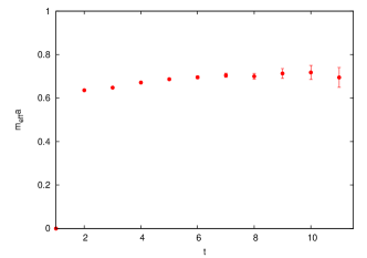
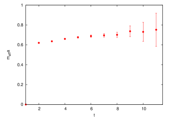
Figure 8: (color online). Effective mass plot corresponding to the simulation at $m_{\pi}^{2}=0.143$ GeV². Only the wall source results are plotted. The point source results are not used in the analysis.

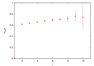
Figure 9: (color online). Effective mass plot corresponding to the simulation at $m_{\pi}^{2}=0.080$ GeV². Only the wall source results are plotted. The point source results are not used in the analysis.

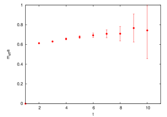
Figure 10: (color online). Effective mass plot corresponding to the simulation at $m_{\pi}^{2}=0.053$ GeV². Only the wall source results are plotted. The point source results are not used in the analysis.

Figure 11: (color online). Effective mass plot corresponding to the simulation at $m_{\pi}^{2}=0.041$ GeV². Only the wall source results are plotted. The point source results are not used in the analysis.

To estimate finite-volume effects using overlap fermions, quenched lattices of volumes $16^{3}\times 28$ and $12^{3}\times 28$ with $a=0.2$ fm are used. For a pion mass of $180$ MeV, $m_{PS}L\approx 3$, and the finite-volume correction is approximately $2.7$ MeV: about $1.5$% of the pion mass Chen et al. (2004). The current $20^{3}\times 32$ lattice with $a=0.153$ fm is about the same physical size as that of a $16^{3}\times 28$ lattice and a similar finite-volume correction is expected. To estimate the finite-volume correction of the lowest $\rho$ meson mass at $m_{\pi}\approx 200$ MeV, the same percentage of error is used, and a shift of $\delta_{L}m_{\rho}\approx 13$ MeV to the $\rho$ mass is calculated for the $\rho$ meson mass of $m_{\rho}\approx 917$ MeV. This is about half of the statistical error of the lattice data. It should be noted that the data that will be used in chiral extrapolations are those with pion mass greater than $400$ MeV, with $m_{PS}L>6.2$. The predictions are extended to the region with pion mass less than $400$ MeV and compared with the lattice data.

With regards to possible lattice artifacts, the lattice results analyzed are based on the overlap fermion on quenched gauge configurations at one lattice spacing. Even though the overlap fermion has relatively smaller $\mathcal{O}(a)$ errors, the $\mathcal{O}(a^{2})$ correction toward the continuum limit has not been taken into account. With a spatial size of $3.06$ fm, $m_{\pi}a\sim 3$ for the smallest pion mass at $200$ MeV is somewhat smaller than $m_{\pi}a=4$, beyond which the finite volume effect has been considered to be small. For $m_{\pi}a\sim 3$, the previous study described in Ref. Chen et al. (2004) estimates that the finite-volume correction is approximately $3\%$ which is smaller than the statistical error of the pion mass.

The enhancement of zero modes effects in QQCD primarily affects the pseodoscalar and scalar mesons. Since all the zero modes appear in one chiral sector in each gauge configuration, the pseodoscalar and scalar mesons will have a leading $1/m^{2}$ singularity from the zero modes. These appear in both the quark and antiquark propagators in the meson correlator Dong et al. (2002). Nevertheless, the vector and axial vector mesons have only a $1/m$ singularity, which is a less dramatic effect. In either case, the quantity that determines the size of the zero mode effects is $m\Sigma V$ in the $p$-regime Leutwyler and Smilga (1992). It has been demonstrated that when $m\Sigma V\gtrsim 5$, the zero mode effect is hardly detectable Chen et al. (2004); Li et al. (2010). For all pion masses displayed in Figure 13, $m\Sigma V>7$. Therefore, there is no reason to suggest that there is a zero mode contribution to the $\rho$ meson correlators being studied.

IV Extrapolation results

IV.1 Renormalization flow curves

In order to produce an extrapolation to each test value of $m_{\pi}^{2}$, a finite-range regularization scale $\Lambda$ must be selected. As an example, one can choose a triple-dipole regulator at $\Lambda=1.0$ GeV. By using Eq.(14), finite- and infinite-volume extrapolations are shown in Figure 13. Note that the $m_{\pi}^{2}$ values selected for the finite-volume extrapolations exactly correspond to the ‘missing’ low-energy data points set aside earlier. The physical point $m_{\pi}^{2}=0.0196$ GeV² is included as well.

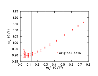
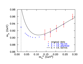
Figure 12: (color online). Quenched lattice QCD data for the $\rho$ meson mass. The dashed vertical line indicates the physical pion mass and the solid vertical line shows how the data set is split into two parts. The lower-mass portion of the data was not known at the time of extrapolation.

Figure 13: (color online). A test extrapolation based on the four lightest original data points (excluding the low-energy set) as shown. Both the finite- and infinite-volume results are shown for a triple-dipole regulator at $\Lambda=1.0$ GeV. The dashed vertical line indicates the physical pion mass.

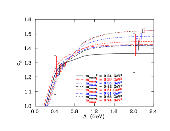
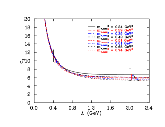
Figure 14: (color online). Behaviour of $c_{0}$ vs. $\Lambda$. A few points are selected to indicate the general size of the statistical error bars.

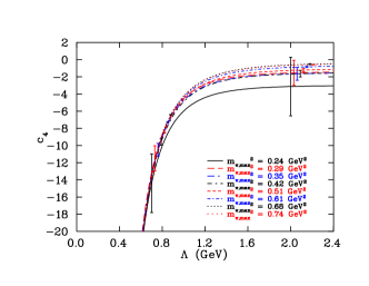
Figure 15: (color online). Behaviour of $c_{2}$ vs. $\Lambda$. A few points are selected to indicate the general size of the statistical error bars.

Figure 16: (color online). Behaviour of $c_{4}$ vs. $\Lambda$. A few points are selected to indicate the general size of the statistical error bars.

Now the regularization scale-dependence of low-energy coefficients $c_{0}$, $c_{2}$ and $c_{4}$ is investigated for various upper limits of the range of pion masses. The renormalization of these low-energy coefficients is considered for a series of $\Lambda$ values. The aim is to obtain renormalization flow curves, each corresponding to a different value of maximum pion mass, $m_{\pi,\mathrm{max}}^{2}$. Thus the behaviour of the renormalization of the low-energy coefficients can be examined as lattice data extend further outside the PCR. Figures 16 through 16 show the renormalization flow curves for each of $c_{0}$, $c_{2}$ and $c_{4}$. Note that each data point plotted has an associated error bar, but for the sake of clarity only a few points are selected to indicate the general size of the statistical error bars. Using the procedure described in Ref. Hall et al. (2010), the optimal regularization scale is identified by the value of $\Lambda$ that minimizes the discrepancies among the renormalization flow curves. This indicates the value of regularization scale at which the renormalization of $c_{0}$, $c_{2}$ and $c_{4}$ is least sensitive to the truncation of the data. Physically, this value of $\Lambda$ can be associated with an intrinsic scale related to the size of the source of the pion cloud.

By examining Figures 16 through 16, increasing $m_{\pi,\mathrm{max}}^{2}$ leads to greater scheme-dependence in the renormalization, since the data sample lies further from the PCR. Complete scheme-independence would be indicated by a horizontal line at the physical point. Since the effective field theory is calculated to a finite chiral order, complete scheme-independence across all possible values of $\Lambda$ will not occur in practice. Note that an asymptotic value is usually observed in the renormalization flow as $\Lambda$ becomes large, indicating that the higher-order terms of the chiral expansion are effectively zero. However, these asymptotic values of the low-energy coefficients are poor estimates of their correct values, as previously demonstrated in a pseudodata model Hall et al. (2010). Instead, the best estimates of the low-energy coefficients lie in the identification of the intersection point of the renormalization flow of the low-energy coefficients. It is also of note that, for small values of $\Lambda$, FRR schemes break down. The regularization scale must be at least large enough to include the chiral physics being studied.

IV.2 Optimal regularization scale

The optimal regularization scale $\Lambda^{\mathrm{scale}}$ can be obtained from the renormalization flow curves using a chi-square analysis described below. In addition, the analysis will allow the extraction of a range for $\Lambda^{\mathrm{scale}}$. Knowing how the data are correlated, the systematic uncertainties from the coupling constants and $\Lambda^{\mathrm{scale}}$ will be combined to obtain an error bar for each extrapolation point. Of particular interest are the values of $m_{\rho,Q}$ at the values of $m_{\pi}^{2}$ explored in the lattice simulations but excluded in the chiral extrapolation.

To obtain a measure of the uncertainty associated with an optimal regularization scale, a $\chi^{2}_{dof}$ function is constructed. This function should allow easy identification of the intersection points in the renormalization flow curves, and a range associated with this central regularization scale. The first step is to plot $\chi^{2}_{dof}$ against a series of $\Lambda$ values. The relevant data are the extracted low-energy coefficients with differing values of $m_{\pi,\mathrm{max}}^{2}$. A plot of $\chi^{2}_{dof}$ is constructed separately for each renormalized coefficient $c$ (with uncertainty $\delta c$):

$$\chi^{2}_{dof}=\frac{1}{n-1}\sum_{i=1}^{n}\frac{{(c(i\,;\Lambda)-c^{T}(\Lambda))}^{2}}{{(\delta c(i\,;\Lambda))}^{2}},$$ (21)

for $i$ corresponding to fits with differing values of $m_{\pi,\mathrm{max}}^{2}$ ($n=8$). The theoretical value $c^{T}$ is given by the weighted mean:

$$c^{T}(\Lambda)=\frac{\sum_{i=1}^{n}c(i\,;\Lambda)/{{(\delta c(i\,;\Lambda))}^{2}}}{\sum_{j=1}^{n}1/{(\delta c(j\,;\Lambda))}^{2}}.$$ (22)

The $\chi^{2}_{dof}$ plots using a triple-dipole regulator are shown in Figures 19 through 19. The optimal regularization scale $\Lambda^{\mathrm{scale}}$ is taken to be the central value $\Lambda_{\mathrm{central}}$ of each plot. The upper and lower bounds obey the condition $\chi^{2}_{dof}<\chi^{2}_{dof,min}+1/(dof)$. The results for the optimal regularization scale and the upper and lower bounds are shown in Table 2. It is remarkable that each low-energy coefficient leads to the same optimal value of $\Lambda$, i.e. $\Lambda_{\mathrm{central}}=0.67$ GeV. By averaging the results among $c_{0}$, $c_{2}$, and $c_{4}$, the optimal regularization scale $\Lambda_{\mathrm{scale}}$ for the quenched $\rho$ meson mass can be calculated for this data set: $\Lambda_{\mathrm{scale}}=0.67^{+0.09}_{-0.08}$ GeV.

The result of the final extrapolation, using the estimate of the optimal regularization scale $\Lambda_{\mathrm{scale}}=0.67^{+0.09}_{-0.08}$ GeV, and using the initial data set to predict the low-energy data points, is shown in Figure 22. The extrapolation to the physical point obtained for this quenched data set is: $m_{\rho,Q}^{\mathrm{ext}}(m_{\pi,\mathrm{phys}}^{2})=0.925^{+0.053}_{-0.049}$ GeV, an uncertainty of less than $6$%.

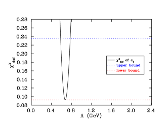
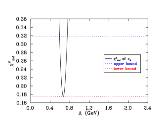
Figure 17: (color online). $\chi^{2}_{dof}$ for $c_{0}$ versus $\Lambda$, corresponding to the renormalization flow curves displayed in Figure 16.

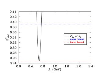
Figure 18: (color online). $\chi^{2}_{dof}$ for $c_{2}$ versus $\Lambda$, corresponding to the renormalization flow curves displayed in Figure 16.

Figure 19: (color online). $\chi^{2}_{dof}$ for $c_{4}$ versus $\Lambda$, corresponding to the renormalization flow curves displayed in Figure 16.

Table 2: Values of the central, upper and lower regularization scales, in GeV, obtained from the $\chi^{2}_{dof}$ analysis of $c_{0}$, $c_{2}$ and $c_{4}$, displayed in Figures 19 through 19.

scale (GeV)	$c_{0}$ (Fig.19)	$c_{2}$ (Fig.19)	$c_{4}$ (Fig.19)
$\Lambda_{\mathrm{central}}$	$0.67$	$0.67$	$0.67$
$\Lambda_{\mathrm{upper}}$	$0.78$	$0.75$	$0.75$
$\Lambda_{\mathrm{lower}}$	$0.58$	$0.59$	$0.60$

Note that each extrapolation point displays two error bars. The inner error bar corresponds to the systematic uncertainty in the parameters only, and the outer error bar corresponds to the systematic and statistical uncertainties of each point added in quadrature. Also, the infinite-volume extrapolation curve is displayed in order to illustrate the effect of finite-volume corrections to the loop integrals.

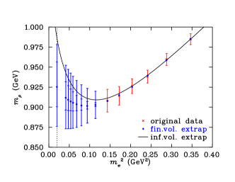
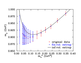
Figure 20: (color online). Extrapolation at $\Lambda_{\mathrm{scale}}=0.67^{+0.09}_{-0.08}$ GeV based on Kentucky Group data, and using the optimal number of data points, corresponding to $\hat{m}_{\pi,\mathrm{max}}^{2}=0.35$ GeV². The inner error bar on the extrapolation points represents purely the systematic error from parameters. The outer error bar represents the systematic and statistical error estimates added in quadrature.

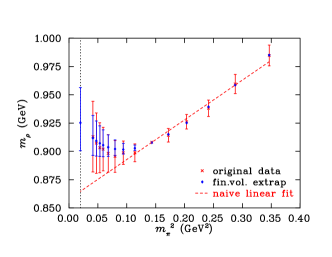
Figure 21: (color online). Comparison of chiral extrapolation predictions (blue diamond) with Kentucky Group data (red cross). Extrapolation is performed at $\Lambda_{\mathrm{scale}}=0.67^{+0.09}_{-0.08}$ GeV, and using the optimal number of data points, corresponding to $\hat{m}_{\pi,\mathrm{max}}^{2}=0.35$ GeV². The inner error bar on the extrapolation points represents purely the systematic error from parameters. The outer error bar represents the systematic and statistical error estimates added in quadrature.

Figure 22: (color online). Comparison of chiral extrapolation predictions (blue diamond) with Kentucky Group data (red cross), with errors correlated relative to the point at $m_{\pi}^{2}=0.143$ GeV². This is done simply to clarify the plot in Figure 22 by removing much of the correlated statistical error. Extrapolation is performed at $\Lambda_{\mathrm{scale}}=0.67^{+0.09}_{-0.08}$ GeV, and using the optimal number of data points, corresponding to $\hat{m}_{\pi,\mathrm{max}}^{2}=0.35$ GeV². The error bar on the extrapolation points represents the systematic error only. A simple linear fit, on the optimal pion mass region, is included for comparison.

In Figure 22, the extrapolation predictions are compared against the actual simulation results, which were not included in the fit. Note that both the extrapolations and the simulation results display the same non-analytic curvature near the physical point. Figure 22 shows the data plotted with error bars correlated relative to the lightest data point in the original set, $m_{\pi}^{2}=0.143$ GeV². This aids in clarifying the plot from Figure 22 by removing much of the correlated statistical error in the lattice data, and allows us to be even more stringent in determining whether the extrapolation is successful. It is notable that the extrapolated results are consistent with the lattice data even after having removed the correlated statistical error. To highlight the importance of this application of an extended $\chi$EFT, a simple linear fit is included in Figure 22. By ignoring low-energy chiral physics, the linear fit is statistically incorrect at the physical point. Note also that all of the missing original data points are consistent within the extrapolations’ systematic uncertainties. After statistical correlations are subtracted, the extrapolated points correspond to an error bar almost half the size of that of the lattice data points. In order to match this precision at low energies, the time required in lattice simulations would increase by approximately four times.

In order to check if scheme-independence is recovered using data within the PCR, the low-energy data that were initially excluded from analysis can now be treated in the same way. That is, renormalization flow curves can be constructed as a function of $\Lambda$ for sequentially increasing $m_{\pi,\mathrm{max}}^{2}$. The results are shown in Figures 25 through 25. Clearly, the renormalization flow curves for each plot corresponding to $c_{0}$, $c_{2}$ and $c_{4}$ are flatter than those of the initial analysis, indicating a reduction in the regularization scale-dependence due to the use of data closer to the PCR. One is not able to extract an optimal regularization scale from these plots, as shown in the behaviour of $\chi^{2}_{dof}$, displayed in Figures 28 through 28. However, each $\chi^{2}_{dof}$ curve provides a lower bound for the regularization scale, where FRR breaks down Hall et al. (2010), as discussed in Section IV.1. These lower bounds are: $\Lambda^{c_{0}}_{\mathrm{lower}}=0.39$ GeV, $\Lambda^{c_{2}}_{\mathrm{lower}}=0.52$ GeV and $\Lambda^{c_{4}}_{\mathrm{lower}}=0.59$ GeV.

The statistical error bars of the low-energy coefficients corresponding to a small number of data points in Figures 25 through 25 is large, and a statistical difference among the curves does not appear until $m_{\pi,\mathrm{max}}^{2}\approx 0.11$ GeV². Thus the identification of an optimal regularization scale will be aided by incorporating data corresponding to even larger values of $m_{\pi,\mathrm{max}}^{2}$. By considering all of the available data, the behaviour of $\chi^{2}_{dof}$, as displayed in Figures 31 through 31, resolve precise optimal regularization scales: $\Lambda^{c_{0}}_{\mathrm{central}}=0.72$ GeV, $\Lambda^{c_{2}}_{\mathrm{central}}=0.71$ GeV and $\Lambda^{c_{4}}_{\mathrm{central}}=0.71$ GeV. The systematic errors obtained from each $\chi^{2}_{dof}$ curve seem arbitrarily constrained as a consequence of including more data points, which extend well outside the chiral regime, and possibly outside the applicable region of FRR techniques. This issue is addressed in the ensuing section.

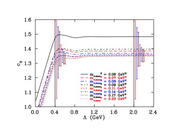
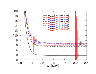
Figure 23: (color online). Behaviour of $c_{0}$ vs. $\Lambda$ including the initially excluded low-energy data. A few points are selected to indicate the general size of the statistical error bars.

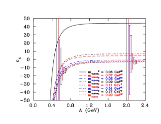
Figure 24: (color online). Behaviour of $c_{2}$ vs. $\Lambda$ including the initially excluded low-energy data. A few points are selected to indicate the general size of the statistical error bars.

Figure 25: (color online). Behaviour of $c_{4}$ vs. $\Lambda$ including the initially excluded low-energy data. A few points are selected to indicate the general size of the statistical error bars.

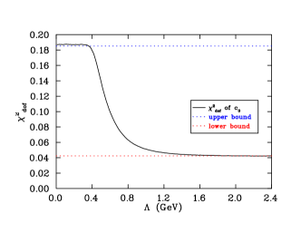
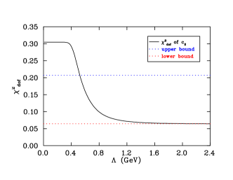
Figure 26: (color online). $\chi^{2}_{dof}$, for $c_{0}$ versus $\Lambda$, corresponding to the renormalization flow curves displayed in Figure 25. A lower bound for the regularization scale is found: $\Lambda^{c_{0}}_{\mathrm{lower}}=0.39$ GeV.

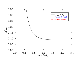
Figure 27: (color online). $\chi^{2}_{dof}$, for $c_{2}$ versus $\Lambda$, corresponding to the renormalization flow curves displayed in Figure 25. A lower bound for the regularization scale is found: $\Lambda^{c_{2}}_{\mathrm{lower}}=0.52$ GeV.

Figure 28: (color online). $\chi^{2}_{dof}$, for $c_{4}$ versus $\Lambda$, corresponding to the renormalization flow curves displayed in Figure 25. A lower bound for the regularization scale is found: $\Lambda^{c_{4}}_{\mathrm{lower}}=0.59$ GeV.

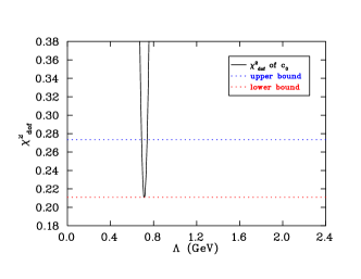
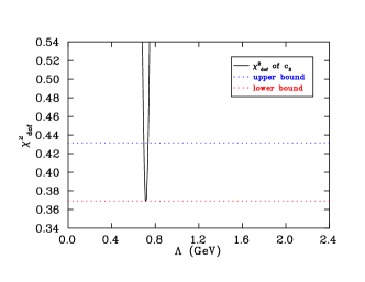
Figure 29: (color online). $\chi^{2}_{dof}$, for $c_{0}$ versus $\Lambda$, corresponding to all available data, including the low-energy set.

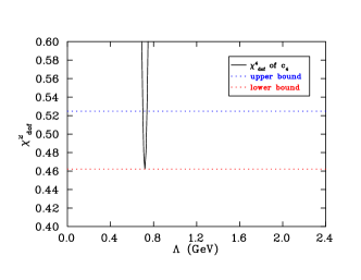
Figure 30: (color online). $\chi^{2}_{dof}$, for $c_{2}$ versus $\Lambda$, corresponding to all available data, including the low-energy set.

Figure 31: (color online). $\chi^{2}_{dof}$, for $c_{4}$ versus $\Lambda$, corresponding to all available data, including the low-energy set.

IV.3 Optimal pion mass region

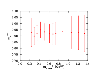
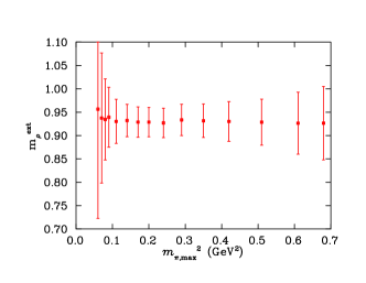
Figure 32: (color online). Behaviour of the extrapolation of the quenched $\rho$ meson mass to the physical point $m_{\rho,Q}^{\mathrm{ext}}(m_{\pi,\mathrm{phys}}^{2})$ vs. $m_{\pi,\mathrm{max}}^{2}$ using the initial data set, which excludes the lowest mass data points. In each case, $c_{0}$ is obtained using the scale $\Lambda_{\mathrm{central}}$ (for a triple-dipole regulator) as obtained from the $\chi^{2}_{dof}$ analysis. The error bars include the statistical and systematic uncertainties in $c_{0}$ added in quadrature. The optimal value $\hat{m}_{\pi,\mathrm{max}}^{2}=0.35$ GeV².

Figure 33: (color online). Behaviour of the extrapolation of the quenched $\rho$ meson mass to the physical point $m_{\rho,Q}^{\mathrm{ext}}(m_{\pi,\mathrm{phys}}^{2})$ vs. $m_{\pi,\mathrm{max}}^{2}$ using the complete data set, which includes the lowest mass data points. In each case, $c_{0}$ is obtained using the scale $\Lambda_{\mathrm{central}}$ (for a triple-dipole regulator) as obtained from the $\chi^{2}_{dof}$ analysis. The error bars include the statistical and systematic uncertainties in $c_{0}$ added in quadrature. The optimal value $\hat{m}_{\pi,\mathrm{max}}^{2}=0.20$ GeV².

In this section, a robust method for determining an optimal range of pion masses is presented. This range corresponds to an optimal number of simulation results to be used for fitting. First, consider the extrapolation of the quenched $\rho$ meson mass, which can now be completed. The statistical uncertainties in the values of $c_{0}$, $c_{2}$, $c_{4}$ are dependent on $m_{\pi,\mathrm{max}}^{2}$. As a consequence, the uncertainty in the extrapolated $\rho$ meson mass $m_{\rho}^{\mathrm{ext}}$ must also be dependent on $m_{\pi,\mathrm{max}}^{2}$. Since the estimate of the statistical uncertainty in an extrapolated point will tend to decrease as more data are included in the fit, one might naïvely choose to use the largest $m_{\pi,\mathrm{max}}^{2}$ value possible in the data set. However, at some large value of $m_{\pi,\mathrm{max}}^{2}$, FRR $\chi$EFT will not provide a valid model for obtaining a suitable fit. At this upper bound of applicability for FRR $\chi$EFT, the uncertainty in an extrapolated point is dominated by the systematic error in the underlying parameters. This is due to a greater scheme-dependence in extrapolations using data extending outside the PCR, meaning that the extrapolations are more sensitive to changes in the parameters of the loop integrals. Thus there is a balance point $m_{\pi,\mathrm{max}}^{2}\!=\hat{m}_{\pi,\mathrm{max}}^{2}$, where the statistical and systematic uncertainties (added in quadrature) in an extrapolation are minimized.

In order to obtain this value $\hat{m}_{\pi,\mathrm{max}}^{2}$, consider the behaviour of the extrapolation of the $\rho$ meson mass to the physical point $m_{\rho,Q}^{\mathrm{ext}}(m_{\pi,\mathrm{phys}}^{2})$, as a function of $m_{\pi,\mathrm{max}}^{2}$. Treating the parameters: $\Lambda^{\mathrm{scale}}$, $g_{2}$, $g_{4}$, $M_{0}^{2}$ and $A_{0}$ as independent, their systematic uncertainties from these sources are added in quadrature. In addition, the systematic uncertainty due to the choice of the regulator functional form is roughly estimated by comparing the results using the double-dipole and the step function. These functional forms are the two most different forms of the various regulators considered, since the dipole was excluded due to the extra non-analytic contributions it introduces. The results for the initial and complete data sets are shown in Figures 33 and 33, respectively. Note that the systematic uncertainty due to $\Lambda^{\mathrm{scale}}$ is included for chiral order $\mathcal{O}(m_{\pi}^{4})$.

Figure 33 indicates an optimal value $\hat{m}_{\pi,\mathrm{max}}^{2}=0.35$ GeV², which will be used in the final extrapolations, in order to check the results of this method with the low-energy data. By using only the data contained in the optimal pion mass region, constrained by $\hat{m}_{\pi,\mathrm{max}}^{2}$, an estimate of the optimal regularization scale may be calculated with a more generous corresponding systematic uncertainty. The value $\Lambda^{\mathrm{scale}}=0.64$ GeV is the average of $\Lambda^{\mathrm{scale}}_{c_{0}}$, $\Lambda^{\mathrm{scale}}_{c_{2}}$ and $\Lambda^{\mathrm{scale}}_{c_{4}}$ using this method. The $\chi^{2}_{dof}$ analysis does not provide an upper or lower bound at this value of $\hat{m}_{\pi,\mathrm{max}}^{2}$. Note that these two estimates of the optimal regularization scale are consistent with each other. Both shall be used and compared in the final analysis. Figure 33 indicates an optimal value $\hat{m}_{\pi,\mathrm{max}}^{2}=0.20$ GeV² for the complete data set, which includes the low-energy data. A higher density of data in the low-energy region serves to decrease the statistical error estimate of extrapolations to the low-energy region. The corresponding value of $\Lambda^{\mathrm{scale}}$ is unconstrained in this case, since the data lie close to the PCR. The breakdown of the systematic error bar into its constituent uncertainties is listed in Table 3.

Table 3: Results for the quenched $\rho$ meson mass for different values of $m_{\pi,\mathrm{max}}^{2}$, extrapolated to the physical point, corresponding to Figures 33 (for the original data set) and 33 (for the complete data set). The uncertainty in $m_{\rho,Q}^{\mathrm{ext}}(m_{\pi,\mathrm{phys}}^{2})$ is provided in the following order: the statistical uncertainty, the systematic uncertainty due to the intrinsic scale, $g_{2}$, $g_{4}$, $M_{0}^{2}$, $A_{0}$ and the regulator functional form, respectively.

$m_{\pi,\mathrm{max}}^{2}$(GeV2)	$m_{\rho,Q}^{\mathrm{ext}}(m_{\pi,\mathrm{phys}}^{2})$ (GeV): original set	$m_{\rho,Q}^{\mathrm{ext}}(m_{\pi,\mathrm{phys}}^{2})$ (GeV): complete set
$0.059$	-	$0.956(234)(1)(0)(0)(1)(0)(0)$
$0.068$	-	$0.938(139)(1)(1)(0)(1)(0)(0)$
$0.080$	-	$0.934(87)(1)(1)(0)(1)(0)(0)$
$0.094$	-	$0.939(64)(2)(1)(0)(1)(0)(1)$
$0.114$	-	$0.930(47)(3)(2)(0)(2)(0)(0)$
$0.143$	-	$0.932(34)(5)(3)(0)(4)(1)(0)$
$0.172$	-	$0.929(31)(6)(4)(0)(5)(1)(0)$
$0.204$	-	$0.929(29)(9)(5)(0)(6)(1)(0)$
$0.241$	$0.930(110)(27)(14)(0)(17)(4)(6)$	$0.927(27)(12)(7)(0)(9)(2)(0)$
$0.288$	$0.899(62)(31)(1)(0)(1)(1)$	$0.933(24)(17)(10)(0)(12)(3)(1)$
$0.347$	$0.922(43)(37)(11)(0)(13)(28)(17)$	$0.932(23)(21)(11)(0)(13)(3)(4)$
$0.422$	$0.948(29)(45)(23)(1)(28)(7)(8)$	$0.930(20)(29)(14)(0)(16)(4)(8)$
$0.515$	$0.932(23)(51)(19)(1)(23)(6)(19)$	$0.929(19)(37)(15)(0)(18)(4)(13)$
$0.610$	$0.921(18)(63)(18)(1)(22)(5)(25)$	$0.926(16)(54)(18)(0)(21)(5)(22)$
$0.676$	$0.915(12)(74)(18)(1)(22)(6)(32)$	$0.926(14)(66)(19)(1)(23)(6)(25)$
$0.743$	$0.919(13)(79)(22)(1)(26)(7)(29)$	$0.922(12)(74)(21)(1)(26)(7)(27)$
$0.867$	$0.933(9)(103)(32)(1)(39)(12)(35)$	$0.923(8)(100)(29)(1)(35)(11)(38)$
$1.062$	$0.928(7)(115)(32)(1)(38)(12)(43)$	-
$1.212$	$0.926(7)(121)(31)(1)(37)(12)(38)$	-
$1.329$	$0.921(6)(132)(31)(1)(37)(12)(43)$	-
$1.742$	$0.915(5)(146)(30)(1)(37)(13)(48)$	-
$2.187$	$0.910(4)(175)(30)(1)(37)(14)(55)$	-
$3.150$	$0.902(3)(197)(29)(1)(36)(14)(61)$	-

Table 4: The values of $c_{0}$, $c_{2}$ and $c_{4}$ as obtained from both the original data set and the complete set, which includes the low-energy data. In each case, the coefficients are evaluated using the scale $\Lambda_{\mathrm{central}}$ (for a triple-dipole regulator) as obtained from the $\chi^{2}_{dof}$ analysis. The value of $m_{\pi,\mathrm{max}}^{2}$ used is that which yields the smallest error bar in adding statistical and systematic uncertainties in quadrature. For the initial data set, $\hat{m}_{\pi,\mathrm{max}}^{2}=0.35$ GeV². For the complete data set, $\hat{m}_{\pi,\mathrm{max}}^{2}=0.20$ GeV². The statistical uncertainty is quoted in the first pair of parentheses, and the systematic uncertainty is quoted due to the parameters, in the following order: $\Lambda^{\mathrm{scale}}$, $g_{2}$, $g_{4}$, $M_{0}^{2}$, $A_{0}$ and the regulator functional form.

	$c_{0}$(GeV2)	$c_{2}$	$c_{4}$(GeV-2)
original set	$1.31(5)(10)(4)(0)(5)(4)(8)$	$7.9(4)(25)(2)(0)(2)(1)(4)$	$-16.2(7)(382)(3)(0)(3)(1)(4)$
complete set	$1.35(4)(3)(36)(16)(60)(166)(113)$	$6.8(5)(17)(13)(1)(17)(14)(11)$	$-3.3(16)(359)(23)(1)(28)(12)(1)$

The values of $c_{0}$, $c_{2}$ and $c_{4}$ for both the original data set and the complete data set are shown in Table 4, with statistical error estimate quoted first and systematic uncertainty due to the parameters $\Lambda^{\mathrm{scale}}$, $g_{2}$, $g_{4}$, $M_{0}^{2}$, $A_{0}$, and the regulator functional form quoted second, in this order. In the case of the original data set, the value of $c_{4}$ is not well-determined, due to the small number of data points used. In the case of the complete data set, the results are dominated by statistical uncertainty and also results in an almost unconstrained value of $c_{4}$. Even if $\Lambda^{\mathrm{scale}}$ is quite well-determined, as observed in Figures 19 through 19, the value of $c_{4}$ itself is sensitive to changes in the regularization scale $\Lambda$, as evident from Figure 16. The coefficients of the complete set are less well-determined due to the fact that $\hat{m}_{\pi,\mathrm{max}}^{2}=0.20$ GeV², leaving only low-energy results with large statistical uncertainties for fitting.

The result using the estimate of the optimal regularization scale $\Lambda^{\mathrm{scale}}=0.64$ GeV, with the systematic uncertainty calculated by varying $\Lambda$ across all suitable values, and using the initial data set, is shown in Figure 35. The extrapolation to the physical point obtained for this quenched data set is: $m_{\rho,Q}^{\mathrm{ext}}(m_{\pi,\mathrm{phys}}^{2})=0.922^{+0.065}_{-0.060}$ GeV, an uncertainty of approximately $7$%. Figure 35 shows the data plotted with error bars correlated relative to the lightest data point in the original set, $m_{\pi}^{2}=0.143$ GeV², using $\Lambda_{\mathrm{scale}}=0.64$ GeV, and varying $\Lambda$ across its full range of values. This naturally increases the estimate of the systematic uncertainty of the extrapolations, but also serves to demonstrate how closely the results from lattice QCD and $\chi$EFT match.

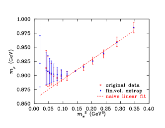
Figure 34: (color online). Comparison of chiral extrapolation predictions (blue diamond) with Kentucky Group data (red cross). Extrapolation is performed at $\Lambda_{\mathrm{scale}}=0.64$ GeV, varied across the whole range of $\Lambda$ values, and using the optimal number of data points, corresponding to $\hat{m}_{\pi,\mathrm{max}}^{2}=0.35$ GeV². The inner error bar on the extrapolation points represents purely the systematic error from parameters. The outer error bar represents the systematic and statistical error estimates added in quadrature.

Figure 35: (color online). Comparison of chiral extrapolation predictions (blue diamond) with Kentucky Group data (red cross), with errors correlated relative to the point at $m_{\pi}^{2}=0.143$ GeV². This is done simply to clarify the plot in Figure 35 by removing much of the correlated statistical error. Extrapolation is performed at $\Lambda_{\mathrm{scale}}=0.64$ GeV, varied across the whole range of $\Lambda$ values, and using the optimal number of data points, corresponding to $\hat{m}_{\pi,\mathrm{max}}^{2}=0.35$ GeV². The error bar on the extrapolation points represents the systematic error only. A simple linear fit, on the optimal pion mass region, is included for comparison.

V Conclusion

A technique for isolating an optimal regularization scale, established in Ref. Hall et al. (2010), was tested in quenched QCD through an examination of the quenched $\rho$ meson mass. The result is a successful extrapolation based on an extended effective field theory procedure. By using quenched lattice QCD results that extended beyond the power-counting regime, an optimal regularization scale was obtained from the renormalization flow of the low-energy coefficients.

An optimal value of the maximum pion mass to be used for fitting was also calculated, and this resulted in an alternative estimate of the value of the optimal regularization scale, which was consistent with the first result. The mass of the $\rho$ meson was calculated in the low-energy region, including the physical point, using each estimate of the optimal regularization scale, and both results were compared. The results of extrapolations using $\chi$EFT, and the results of lattice QCD simulations, were demonstrated to be consistent. The extrapolation correctly predicts the low-energy curvature that was observed when the low-energy lattice simulation results were revealed.

In full QCD, using dynamical fermions, the process $\rho\rightarrow\pi\pi$ contributes to the $\rho$ meson mass. This means that near the chiral limit, the $\pi\pi$ component of the $\rho$ necessarily involves a hard momentum scale, and therefore is not amenable to the standard methods of low-energy expansions, as entailed by $\chi$PT. Therefore, one needs to resort to alternative techniques in such instances.

However, since there exists no experimental value for the mass of a particle in the quenched approximation, this analysis demonstrates the ability of the technique to make predictions without phenomenologically motivated bias. The results clearly indicate a successful procedure for using lattice QCD data outside the power-counting regime to extrapolate an observable to the chiral regime.