Efficient quantum computing with weak measurements

Abstract

Projective measurements with high quantum efficiency is often assumed to be required for efficient circuit based quantum computing. We argue that this is not the case and show that this fact has actually be known previously though not deeply explored. We examine this issue by giving an example of how to perform the quantum ordering finding algorithm efficiently using non-local weak measurements given that the measurements used are of bounded weakness and some fixed but arbitrary probability of success less than unity is required. We also show that it is possible to perform the same computation with only local weak measurements but this must necessarily introduce an exponential overhead.

1 Introduction

The work of DiVincenzo [1] states explicit requirements for scalable circuit based quantum computing. Given the current state of art, meeting these requirements in even moderately sized systems is technologically challenging ([2] and references therein). With some more modern implementations the criteria can be difficult to apply, but some reinterpreted set of criteria will apply for any particular implementation [2]. DiVincenzo’s requirements consist of five criteria: well defined scalable qubits, the ability to prepare fiducial states, near perfect (below fault tolerant threshold) unitary evolution, access to a universal set of unitary evolutions and near perfect quantum measurement.

There exists an assumption that the measurement criteria requires strong projective measurements with near unit quantum efficiency to achieve the efficiency possible in quantum computing [3]. This may seem reasonable given that proposed quantum algorithms which are efficient compared to the best known classical algorithms are presented with measurements in the basis of the eigenstates of Hermitian operators. Furthermore, models of quantum computing such as cluster state quantum computing [4] rely on strong measurements to perform the required state transformations for universal computation. However, as DiVincenzo mentions [1], this is not a strict requirement and one can make trade-offs between conditions to achieve scalable quantum computing. The important issue is if when making a trade-off that algorithmic efficiency is not lost.

This work is motivated by this brief observation of DiVincenzo to explicitly show a non-trivial example of an efficient quantum algorithm which involves non-ideal, and in particular, weak quantum measurements [5]. As a result, we hope to demonstrate in theory that when building a demonstration quantum computer based on the circuit model, strong projective measurement for read-out in the computational basis is not absolutely necessary. This is an important consideration when constructing small to medium scale quantum computers as it allows for an extra degree of freedom which can assist in the the design of algorithms matched to the strengths of the particular architecture used.

In this work we will consider working in an architecture that is constrained in such a way as the interaction strengths for the readout measurements will only vary over a very small range and the time taken for the measurement is limited to small values to minimise the effects of decoherence. Within this constraint there has been some work to speed-up the measurement process by adapting parameters as the measurement proceeds [6]. Here we will consider working in a non-adaptive regime and allow for arbitrary small (but bounded) measurement strengths. As the information gained in each measurement is small the results from any algorithms must necessary be formed by processing over an ensemble. The situation we will consider is distinct from the situation found for bulk ensemble nuclear magnetic resonance quantum computing [7] as we will still require the preparation of pure quantum states before the computation.

Our paper is ordered as follows: In the first section we will describe weak measurements following the standard presentation given in recent literature. Then we will then review a specific type of weak measurement on qubits which differs slightly to the standard presentation but will be useful for our purposes. In the second section we will describe how to use this weak measurements in quantum computing and give two specific examples of algorithms which may utilise such measurements. The two examples will be of the satisfiability and order finding algorithms which we will show lead to a respective inefficient and efficient use of weak measurements in quantum algorithms. In the penultimate section we will discuss the potential use of fault tolerant constructions within this model and the how using local weak measurements generally results in an inefficient overhead. Finally we will conclude our results.

2 Weak Measurements

Aharonov, Albert and Vaidman (AAV) [5] shows how one can make a ”weak” measurement of an observable $A$ in which any single measurement outcome from the apparatus has very little information about the value of $A$ and is hence very noisy. However, averaging over a large enough ensemble this noise can be removed and averages of $A$ can be recovered. It is possible to construct the measurement so that the lower the information gathered about $A$ the less the system is disturbed. Quantum mechanics allows this disturbance to go to zero as the information obtained for $A$ goes to zero [8]. However, as the measurement becomes weaker larger ensembles are required to mitigate the effects of the noise and maintain a desired precision for the average of $A$.

AAV consider a measurement model with a system Hilbert space and a separate apparatus Hilbert space which describes the measuring apparatus. The apparatus space is assumed to have the same structure as a harmonic oscillator and the observable $X$ will represent the measurement outcomes and $P_{x}$ will be the generator of infinitesimal translations in $X$. The apparatus is also assumed to be in an initial state which is Gaussian and separable from the system. The system and apparatus are coupled by a Hamiltonian $H=gA\otimes P_{x}$ where $A$ is the observable that we wish to weakly measure and $g$ is a scalar value which will be a factor in determining the strength of the measurement. The observable $A$ can be any observable on the system. A system which is strongly isolated will have small values for the coupling constants in the Hamiltonian.

In the Heisenberg picture, the apparatus observable $X$ evolves to $X+gtA$ where $t$ is the interaction time for the coupling between the system and apparatus. Knowing the strength and duration of the coupling and the initial state of the apparatus gives sufficient information for the statistics of $A$ to be calculated from the measurement results from the apparatus alone irrespective of the strengths of the interaction. However, weaker measurements will require more measurements if some bound on the uncertainty in the statistical estimators is required to be achieved.

2.1 Projector probability observables

Projection operators are valid observables. The expectation value of such a projector observable is the modulus squared length of the component of the state within the subspace of the projector. In other words, if the projector is constructed from the space spanned by eigenstates of an observable with particular eigenvalue, then the expectation value of the projector is the same as the probability that a strong measurement of the observable would result in that eigenvalue had it been made on the same ensemble. This idea of projectors as probability operators follows naturally from the generalised theory of quantum measurement.

If one can make a weak measurement of this projector observable then it is possible to obtain this probability without actually having to actually perform the strong measurement of the underlying observable or greatly disturbing the system.

Finding a system with a Hamiltonian of the right form for a projector observable might be difficult, but one can use the quantum computing circuit model to construct a device which does with the system and apparatus both qubits [9, 10, 11]. This construction is not the same as that considered in AAV, but of the same flavour. We will now describe this construction of a qubit weak measurement of a projector observable.

2.2 Single-qubit measurement model

Consider a measurement with the system and apparatus Hilbert spaces both a single qubit. The system is assumed to be prepared in an arbitrary state $\ket{\Psi}$ and the apparatus is prepared in a pure state $\cos\theta\ket{0}+\sin\theta\ket{1}$ uncorrelated with the system (i.e. a separable state). Instead of specifying a Hamiltonian we will specify the coupling of the system and apparatus by a unitary gate, in particular the controlled NOT (CNOT) operation. Finally the apparatus will be observed with the $Z=\ket{0}\bra{0}-\ket{1}\bra{1}$ observable. This configuration is depicted in black in Figure 1.

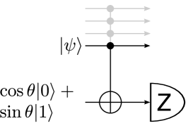
Figure 1: Model of a qubit based weak measurement. An apparatus (the lowest shown qubit) is prepared in the state $\cos\theta\ket{0}+\sin\theta\ket{1}$ and measured in the $Z$ basis after interacting with the system (the upper qubits) prepared in an arbitrary state $\ket{\psi}$. The black lines shows the case of a single qubit weak measurement in which the interaction between the system and meter is of the form of a singly controlled not gate. The black and grey lines combined show the general many qubit case of a multi-controlled not gate. The weakness of the measurement is determined by the parameter $\theta$ where for $\cos\theta=1$ the measurement is strong and equivalent to a projective measurement and where $\cos\theta=1/\sqrt{2}$ the measurement is completely turned off. See text for details.

If the $Z$ measurement of the apparatus is propagated back through the CNOT (c.f Heisenberg picture) then the final measurement of the apparatus is equivalent to a measurement of $Z\otimes Z$ on the system and apparatus before the interaction. In other words, the measurement is equivalent to a measurement of the parity subspace on the combined input state. If the system state is written $\ket{\Psi}=\alpha\ket{0}+\beta\ket{1}$ then the probabilities for the two measurement results will be

$$P(+) = |\alpha|^{2}\cos^{2}\theta+|\beta|^{2}\sin^{2}\theta$$ (1)

$$P(-) = |\alpha|^{2}\sin^{2}\theta+|\beta|^{2}\cos^{2}\theta.$$ (2)

From these equations it is possible to see that for $\theta=0$, the measurement output will be equivalent to a projective $Z$ measurement on the system. For $\theta=\pi/4$ then the output will give either result with equal probability independent of the system state. It is possible to show that when $\theta=\pi/4$ the state of the system is undisturbed. This is unlike the AAV model in which the strength of the interaction is tuned not only from the initial meter state, but by the strength of the interaction in the Hamiltonian and the interaction time. Here the full range of possible measurement strengths are achieved by tuning the initial meter state. However, one can think of this model as a $Z$ measurement on the system of the AAV type.

The average value for $Z$ can be found from the expectation value of the function $\tilde{Z}$ defined by

$$\tilde{Z}(x=+) = \frac{1}{\cos^{2}\theta-\sin^{2}\theta}$$ (3)

$$\tilde{Z}(x=-) = -\frac{1}{\cos^{2}\theta-\sin^{2}\theta}$$ (4)

where $x$ is the meter measurement result. This function is well defined for $\theta\in[0,\pi/4)$. The variance of this function on a single measurement is given by

$$\frac{1}{(\cos^{2}\theta-\sin^{2}\theta)^{2}}-(|\alpha|^{2}-|\beta|^{2})^{2}.$$ (5)

The variance can be understood as having a contribution of $(\cos^{2}\theta-\sin^{2}\theta)^{-2}-1$ from the variance due to the weakness of the measurement which can be infinitely large and $1-(|\alpha|^{2}-|\beta|^{2})^{2}$ from the variance of the system state which is at most $1$. For weak measurements the variance in the output is dominated by the variance due to the weakness of the measurement. This statement can be taken as a quantitative definition of measurement weakness.

It is possible to make a measurement of the expectation value of the projector onto the $+1$ subspace of the $Z$ operator by the same apparatus but calculating the expectation value of the function

$$\tilde{\Pi}_{Z}(x=+) = \frac{1}{2}+\frac{1}{2(\cos^{2}\theta-\sin^{2}\theta)}$$ (6)

$$\tilde{\Pi}_{Z}(x=-) = \frac{1}{2}-\frac{1}{2(\cos^{2}\theta-\sin^{2}\theta)}$$ (7)

which has a mean of $|\alpha|^{2}$ for all theta except $\pi/4$ and a variance of

$$\frac{1}{4(\cos^{2}\theta-\sin^{2}\theta)^{2}}-\frac{(|\alpha|^{2}-|\beta|^{2})^{2}}{4}.$$ (8)

A similar analysis of the contributions to the variance can be made as above.

2.3 Multi-qubit measurements

It is possible to extend this construction to build a larger class of weak measurement of projectors using multiply controlled NOT gates. This configuration is depicted in the combined black and grey schematic in Figure 1. Multiply controlled NOT gates can be built efficiently using $O(n^{2})$ singly controlled gates and local unitaries [14]. A measurement of $Z$ on the meter after the interaction is equivalent to a measurement of the operator

$$\hat{P}_{\bot}\otimes\ket{0}\bra{0}+\ket{111\cdots}\bra{111\cdots}\otimes\ket{1}\bra{1}-$$

$$\hat{P}_{\bot}\otimes\ket{1}\bra{1}-\ket{111\cdots}\bra{111\cdots}\otimes\ket{0}\bra{0}$$ (9)

on the system and meter Hilbert spaces before the interaction where $\hat{P}_{\bot}$ is the projector onto the subspace which is the complement of the all ones subspace (i.e. the subspace which is spanned by all qubit basis states except $\ket{1111\cdots 1}$).

If the apparatus is prepared the as in the case with a single control and the system is in the state $\ket{\psi}$ then the probability of the two outcomes of the apparatus measurement are

$$P(+) = \bra{\psi}\hat{P}_{\bot}\ket{\psi}\cos^{2}\theta+|\braket{111\cdots}{\psi}|^{2}\sin^{2}\theta$$ (10)

$$P(-) = \bra{\psi}\hat{P}_{\bot}\ket{\psi}\sin^{2}\theta+|\braket{111\cdots}{\psi}|^{2}\cos^{2}\theta.$$ (11)

This distribution is the same as with the singly controlled CNOT gate but with the probabilities for the qubit in the system being in the one state replaced by the expectation values of the projectors onto the space with all ones. The mean and variances as calculated above also follow this replacement of variables. Therefore the nature of the statistics do not change as the input size of the system Hilbert space increases.

2.4 Measuring probabilities in the computational basis

This model can also be used to measure the expectation value of projectors onto any one dimensional subspace generated by a particular computational basis state by placing $X=\ket{0}\bra{1}+\ket{1}\bra{0}$ gates before the measurement to transform the desired subspace into the all ones subspace.

The value of the probability can be read out from the data collected at the meter by calculating the expectation value for the estimator of the average of the projection operator given above. Using the assumption of a weak measurement and large sample sizes, we can apply the central limit theorem to the estimator for the probability to calculate the uncertainty in the estimate of the expectation value. With some fixed error probability $\epsilon$ the estimate confidence interval is symmetric around the mean value and has width

$$2\sqrt{2}\frac{\sigma}{\sqrt{M}}\mathrm{erf}^{-1}\left(1-\epsilon\right)\leq\frac{\mathrm{erf}^{-1}\left(1-\epsilon\right)}{\sqrt{2M}(\cos^{2}\theta-\sin^{2}\theta)}$$ (12)

where $\sigma$ is the standard deviation of the measurement results, $M$ is the number of measurements made and $\mathrm{erf}$ is the standard error function.

Measuring the projectors spanned by multiple computational basis states can be simplified for some particular combinations of states. If the states contain all combinations of particular qubits with all other qubits constant, then the qubits which vary can simply be not measured. However, if even a single qubit combination is missing then each combination must be measured separately.

3 Algorithms with weak measurements

In this section we are going to describe quantum computing algorithms in terms of the expectation values and decision problems but analyse the complexity by restricting ourselves to the qubit weak measurement just described.

3.1 Algorithmic complexity

It is assumed that there is some (presumably small) fixed error tolerance allowed for the computation as a whole. For algorithms utilising the weak qubit measurement readout just described, the temporal computational complexity is then determined by how many repetitions are required to achieve this error value. If under these conditions the quantum algorithm has a polynomial temporal complexity it is in the BQP complexity class (the class of practical quantum problems).

We are going to assume that the strength of all measurements is well known and greater than some fixed constant value. Hence a worst case value is known for the uncertainty in the output measurement statistics and we will assume this worst case value is the actual estimate for the uncertainty. We are also going to assume that sample sizes are large enough that the central limit theorem applies. We are not going to be dealing with any distributions in which the central limit theorem is not valid. These assumptions combined allows the variance of the sample mean to be computed and hence a signal to noise ratio involving the estimated mean and the worse case standard deviation can be used to infer the maximum probability of error inherent in the computation.

3.2 Satisfiability with expectation values

The satisfiability problem is defined as identifying if a logical statement described by a Boolean function $f$ has a set of inputs which result in the function evaluating to true. If the function represents a conjunction of logical statements (the inputs), then the statement (the output) is said to be satisfied by the particular combination of truth values used to achieve this output. This problem is in the class of decision problems.

Cory et al. [12] construct a quantum algorithm for solving the satisfiability problem. In their paper they assumed that the standard model of quantum computing is enhanced by special measurements which can extract expectation values of observables for a single instance of a quantum state in an error and noise free way. Their work was motivated by the Nuclear Magnetic Resonance quantum computing model so this type of measurement involving ensemble averages is a natural consequence of the output signals from that type of computation. They then show that given an equal superposition of all possible logical inputs to the function, of which there are $2^{n}$ possibilities, a unitary which implements $f$ can be built efficiently and evaluates all of these possibilities coherently in superposition. The unitary is built so that the output value of the function is written onto another qubit register which is zero if the input does not satisfy the statement and one if it does. The expectation value of the output register is then obtained using the special measurement which they added as described above. If the expectation value is non-zero then the logical statement is satisfiable. Though this does not say which input will satisfy the function, it does show that such a satisfying input exists. Provided one has this enhancement which allows for the immediate extraction of expectation values this is a method of solving an NP-complete problem (i.e. satisfiability) deterministically in polynomial time.

This result is only possible when neglecting the noise in the output of such a measurement. If one requires this measurement to be a standard quantum measurement rather than the special one used, then the complexity will change as more measurements are required to counter the effects of the noise. Consider the possible case of where only a single particular input satisfies the function (as is possible for any size satisfiability problem). The measurement then needs to distinguish between the two cases of being unsatisfiable and the output register in the state $\ket{0}$ and the case of having a single satisfying input and the output register is in the state $(1-2^{-n})\ket{0}\bra{0}+2^{-n}\ket{1}\bra{1}$. The probability to be estimated is then of size $2^{-n}$ and in the large $M$ limit the noise is $2^{-n/2}/\sqrt{M}$ and hence the signal to noise ratio decreases exponentially in the size of the input. This overcomes the apparent speed-up offered by the enhanced model of quantum computing considered as the sample size needed to achieve a particular probability of error in the decision problem will increase exponentially.

As we show next, not all useful ensemble averages from the output of quantum computations necessarily have this problem.

3.3 Order finding with expectation values

The order finding problem is a critical part of the quantum prime factorisation algorithm [13]. The definition of the order finding problem is given positive integers $N$ and $x<N$ find the least positive integer $r$ such that $x^{r}=1(modN)$. This problem is an instance of the hidden subgroup problem which is a more general class of problems [14]. The problem of factoring integers can be reduced to this problem [14]. Currently, the best known classical algorithms have exponential complexity.

The quantum order finding algorithm utilises a quantum modular exponentiation operation defined by the unitary

$$U_{x,N}=\ket{y}=\ket{xy(modN)}$$ (13)

which can be done efficiently using $O(n^{3})$ gates where n is the number of bits needed to represent integers up to $N$. The eigenvalues of this unitary are $exp(2\pi is/r)$ where $r$ is the order of $N$ and $s$ is an integer satisfying $0\leq s<r$ which labels each of the eigenstates. Therefore performing quantum phase estimation on an eigenstate of the modular exponentiation operator is a method of finding information about the order of $x$ [14]. However preparing the eigenstate would require that the order of the integer of interest be known already. Therefore, a superposition state of all possible eigenstates is used. This state happens to be equal to a state that is the representation of the multiplicative identity in the computational basis. Therefore, the output of the order finding algorithm is a phase $\phi=s/r$ where $r$ is the order that we desire and $s$ is equally distributed amongst the allowed values. The continued fractions expansion of $\phi$ allows for the computation of values for $r$. However, if $s$ and $r$ share a factor, then this method will give the value of $r$ with this factor divided out. This is then not the order that was desired but a factor of the order.

For a randomly selected value of $s$ the probability that it is prime for large values of $N$ is at least and will asymptotically approach

$$\frac{1}{2\log N}\geq\frac{1}{n(2\log 2)}.$$ (14)

This guarantees that there will be some probability that the correct answer is contained within the output and that this probability drops as $\Omega(n^{-1})$ with the size of the problem. An example of the distribution for values of $r$ read out from the continued fractions algorithm is shown in Figure 2.

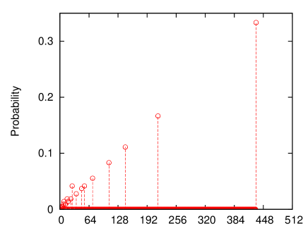
Figure 2: An example distribution of output values for the denominator register when the order is known to be $432$. If the order is prime then all of the probability is concentrated at the highest value.

We are now in a position to describe the quantum order finding algorithm using only weak measurements. The procedure that will be described here is also shown schematically in Figure 3. First, build the order finding algorithm as done for projective readout measurement, but do not measure the register containing the phase $\phi=s/r$ result. This requires no projective measurements only good state preparation and precise unitary evolution. Second, implement the continued fractions algorithm and calculate the rational convergent on the $s/r$ register in the computational basis quantum mechanically using a construction based upon universal reversible gates [14]. This construction requires no measurement or feed-forward, but does require a multi-qubit conditional unitaries. This shifts $O(n^{3})$ classical gates to quantum gates and represents part of the overhead to this method. Tracing over the numerator, the reduced density operator for the convergent’s denominator register will be

$$p\ket{\Psi}\bra{\Psi}+(1-p)\hat{\rho}_{e}$$ (15)

where $\ket{\Psi}$ is the state of the denominator register representing $r$ (the result). $\hat{\rho}_{e}$ is a density operator orthogonal to $\ket{\Psi}$ representing those terms when the numerator had a common factor with the denominator. The standard procedure for the readout is to make a strong projective measurement on this state in the computational basis to read out a result, test to see if it is a solution and repeat the algorithm (possibly modified) if the order if found not to be correct but a factor of the order. Here, we wish to only use weak measurements to extract the answer. It is clear that the largest value of any component from the denominator register will be the order we are seeking and not merely a factor of the order. Therefore we propose to extract the register state with the largest numerical value through a bi-sectional search on properties of denominator register using ensemble averages.

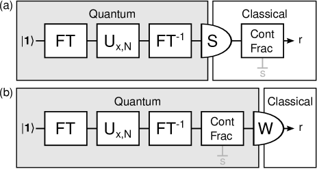
Figure 3: Schematic diagrams showing the difference between the strong (a) and weak (b) measurement versions of the ordering finding algorithm. FT represents the Fourier transform unitary and the unitary $U_{x,N}$ is defined in the text. S and W represent strong and weak measurement read-out respectively. The continued fraction algorithm as utilised for this order finding algorithm has two outputs, the numerator represented by $s$ and whose information is not utilised, and the denominator register represented by $r$. They key distinction is that in this presentation the continued fractions algorithm is performed quantum mechanically in the weak measurement version.

The bi-sectional search proceeds by a series of decision problems. The problems form the answer bit by bit generating the largest value with non-zero probability from the most significant bit to the least significant bit. These probabilities are extracted by taking expectation values of carefully selected projectors as we will now detail. Consider the projector onto the space containing a logical one state for the most significant qubit of the denominator register and all other registers allowed any value. This projector is

$$\hat{\Pi}_{1...}=\frac{1}{2}(Z-I)\otimes I\otimes I\otimes\ldots.$$ (16)

If the average of this projector was non-zero, then it is known that the largest numerical value in the computational basis for the denominator register state have its most significant bit as a 1. If the average is zero then the largest value must have a zero for the most significant bit. This procedure is this repeated for the next most significant bit using the appropriate projector adapted from the previous result. For example, if the most significant bit was a zero, then the next measurement to be made would be

$$\hat{\Pi}_{01...}=\frac{1}{2}(Z+I)\otimes\frac{1}{2}(Z-I)\otimes I\otimes\ldots$$ (17)

or if it was a one then the next measurement is

$$\hat{\Pi}_{11...}=\frac{1}{2}(Z-I)\otimes\frac{1}{2}(Z-I)\otimes I\otimes\ldots.$$ (18)

This continues for each bit and when all have been read out the largest value with non-zero probability for the register is known. At each step the projector representing the space containing the answer has it’s dimension halved however the size of the expectation value is bounded by the probability given in Eq. 14. An illustration of how the bi-sectional search works is shown in Figure 4.

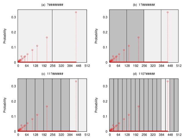
Figure 4: An illustration of the steps involved for the bi-sectional search for the read out of the largest value of the register with non-zero probability. The distribution chosen is the same as Figure 2, hence the answer read out should be a binary representation of $432$ ($110110000$). Initially the most significant bit is weakly measured, the remaining qubits are not measured and their values are not yet known. This state of knowledge is shown in the title of the plot of part (a) with $\#$ representing unknown information that is not to be measured and $?$ representing unknown information that is currently being measured. The weak qubit measurement described in the text is used to determined if there is any probability of the most significant bit value being one. The measurement is equivalent to determining if there is any probability on the right hand side of the plot as shown by the central dividing line. If there is any probability that the state is one (as is the case here), then the measurement proceeds to determining if there is any probability in the output within the $\ket{11}$ subspace as depicted in part (b). If there was, then the measurement proceeds to determining if there is any probability in the $\ket{01}$ state. This repeats until all qubits are measured and the final read out value will be the largest non-zero probability value within the qubit register. If there are $n$ qubits then this procedure has $n$ steps.

To achieve an overall algorithmic error probability less than $\epsilon$, the error probabilities for each bit readout measurement must be less than $\epsilon/n$. This is because if the probability of failure for one run is $\epsilon^{\prime}$ then the overall probability of failure is $1-(1-\epsilon^{\prime})^{n}<n\epsilon^{\prime}$ and hence $n\epsilon^{\prime}<\epsilon$. If we invoke the central limit theorem as foreshadowed above and assume that the estimator for the mean is normally distributed with a variance of $\sigma_{0}^{2}/n$ with $\sigma_{0}$ being the variance in a single outcome and we are deciding between two means of $s_{0}$ and $s_{1}$ (which we will call the signal), then we define $\mathrm{SNR}_{0}=|s_{1}-s_{0}|/\sigma_{0}$. Here we are assuming that the variance from the two distributions is equal. We can do this by choosing a worse case variance as described above. Taking a threshold half way between the two signal values, the probability of making an error is

$$P_{\mathrm{error}}=1-\Phi\left(\frac{\mathrm{SNR}_{0}\sqrt{M}}{2\sqrt{2}}\right)$$ (19)

where $\Phi$ is the cumulative distribution function of the standard normal distribution. We require this probability to be less than $\epsilon^{\prime}=\epsilon/n$. The number of samples required to meet the error budget must therefore satisfy

$$M=\left[\frac{2\sqrt{2}}{\mathrm{SNR}_{0}}\mathrm{erf}^{-1}\left(1-\frac{2\epsilon}{n}\right)\right]^{2}$$ (20)

which scales poly-logarithmically in $n$ for the bi-sectional search alogrithm. To prove this scaling, rearranging this expression gives

$$\mathrm{erf}\left(\frac{\mathrm{SNR}_{0}\sqrt{M}}{2\sqrt{2}}\right)=1-\frac{2\epsilon}{n},$$ (21)

which is equivalent to

$$\frac{\epsilon}{n}=\frac{1}{\sqrt{\pi}}\int_{\mathrm{SNR}_{0}\sqrt{N}/2\sqrt{2}}^{\infty}e^{-t^{2}}\mathrm{d}t.$$ (22)

For $M$ sufficiently large (in particular $\mathrm{SNR}_{0}\sqrt{M}>2\sqrt{2}$)

$$\int_{\mathrm{SNR}_{0}\sqrt{M}/2\sqrt{2}}^{\infty}e^{-t^{2}}\mathrm{d}t < \int_{\mathrm{SNR}_{0}\sqrt{M}/2\sqrt{2}}^{\infty}e^{-t}\mathrm{d}t$$ (23)

$$= e^{-\mathrm{SNR}_{0}\sqrt{M}/2\sqrt{2}}.$$

Therefore

$$n>\epsilon\sqrt{\pi}e^{\mathrm{SNR}_{0}\sqrt{M}/2\sqrt{2}}$$ (24)

or rearranging

$$\sqrt{M}<\frac{2\sqrt{2}}{\mathrm{SNR}_{0}}(\log n-\log\epsilon\sqrt{\pi})$$ (25)

and therefore

$$\left[\frac{2\sqrt{2}}{\mathrm{SNR}_{0}}\mathrm{erf}^{-1}\left(1-\frac{2\epsilon}{n}\right)\right]^{2}=O(n\log(n)^{2})$$ (26)

where we have used the $\Omega(n^{-1})$ scaling of $\mathrm{SNR}_{0}$ from equation 14. Therefore the number of total weak measurement samples needed in the algorithm is $\Omega(n\log(n)^{2})$.

This requirement to make poly-logarithmically extra samples forms another part to the overhead of this procedure. Furthermore, the multiplying factor in the scaling will depend on the weakness of the measurement which may be large for very weak measurements. However, none of the overheads introduced in this presentation scale exponentially in the size of the input.

4 Discussion

4.1 Local weak measurements

Resch and Steinberg [15] have shown that it is possible to extract non-local weak values from local weak measurements. Therefore, one might be tempted to measure the multi-qubit expectation value using local single-qubit measurements instead of the non-local measurements used here. However this does introduce an inefficient overhead.

In general, measuring an $n$ qubit output will need to have estimates of the expectation values for observables of the form $A_{1}A_{2}\cdots A_{n}$. When observing the correlations in the local meter readouts to estimate this value, the variance of the correlation constructed from all the meters is

$$var(X_{1}X_{2}...X_{n})_{o}=\langle(X_{1}X_{2}...X_{n})^{2}\rangle_{o}-\langle X_{1}X_{2}...X_{n}\rangle_{o}^{2},$$ (27)

where $X$ represents the meter observables as per section 2 and the subscript $o$ is a reminder that this description is for measurements at the meter output. If each meter is initialised separately with a mean of zero and a variance of $\sigma^{2}$ then the variance at the meter output in terms of the inputs becomes

$$var(X_{1}X_{2}\cdots X_{n})_{o} = \langle(X_{1}+\gamma A_{1})^{2}(X_{2}+\gamma A_{2})^{2}\cdots(X_{n}+\gamma A_{n})^{2}\rangle_{i}$$ (29)

$$-\gamma^{2n}\langle A_{1}A_{2}...A_{n}\rangle_{i}^{2}$$

$$= \sigma^{2n}+\gamma^{2}\sigma^{2(n-1)}\sum_{k=0}^{n}\langle A_{k}^{2}\rangle_{i}+$$

$$\gamma^{4}\sigma^{2(n-2)}\sum_{k=0}^{n}\sum_{l=0}^{n}\langle A_{k}^{2}A_{l}^{2}\rangle_{i}+\cdots+$$

$$\gamma^{2n}var(A_{1}A_{2}\cdots A_{n}).$$

where we have used the commutativity of the different subsystems to rearrange terms and statistical independence of the meters and the meter and system to remove terms. This expression has a scaling of $O(\sigma^{2n})$ from the first term on the right hand side which is independent from the actual signal from the system observable. Therefore the $\mathrm{SNR}_{0}$ term, instead of being constant as is the case above, decreases exponentially entirely removing the efficiency of the algorithm presented.

Observables of the type just mentioned are observed locally in the standard presentation of quantum computing algorithms using strong measurements. Clearly there must be a point of transition in the initial variance of the meter states compared to the measurement strength where the exponential scaling term from the meter noise does not play a significant role in the data extraction. This quantity will be dependent on the observables needed and hence the type of algorithm being implemented. For example a fault tolerant implementation would have a point in which the noise scaling reduces as the size of the observables increased rather than increasing as is the case in this simple example.

Another possible way to avoid this problem of local weak measurement introducing an exponential overhead is to break the requirement of local preparation of initial meter states. If the initial meter state was correlated then the equality reached above would change significantly. If the right state is chosen for the observable of interest then it may be possible to avoid the exponential scaling.

Other work on non-local weak measurements in a completely different context has also found that estimating non-local correlations is inefficient and requires large ensembles [16, 17]. So it appears that for efficient quantum information processing with weak measurements, non-locality is strictly required. This means that schemes for extracting conditional expectation values using informationaly complete but not full strength measurements [20] cannot be used to perform efficient computation.

4.2 Decoherence times

One may argue that the weakness of the readout and the length of time for the output for the algorithm counteract one another. However, this is not true for the algorithm presented here as the algorithm is rerun, qubits are reprepared and the unitary evolution is run again, which removes any of the effects of previous decoherence. Hence the important time to consider is decoherence over the time taken to execute all the operations needed to run the algorithm in total just is the case for strong measurements. With the standard model of weak measurements (as presented here and in [5]) the interaction time for a weak measurement is much smaller than that for the corresponding strong measurement and hence could act to reduce the effects of decoherence.

4.3 Fault Tolerance

Fault tolerance encoding, evolution and decoding can still be performed if the final measurements are not strong measurements. For the CSS class of quantum codes one can avoid using measurements completely and still achieve fault tolerance [18]. Doing so involves some penalty in the fault tolerant threshold, but as shown recently this penalty is not as great as has been believe previously [19].

4.4 Implications for experimental implementation of quantum computing

This result suggests that in the pursuit of preliminary or proof-of-principle quantum computing experiments that strong isolation and high fidelity operations are where effort should focus provided one has the ability to readout data even if very noisy. For the order finding algorithm presented here, having a weak readout does not harm the efficiency of quantum computing. Increasing the strength of the readout clearly has an advantage in the rate at which computation can occur, but this should not be done to the detriment of the ability for the data to be preserved within the quantum computer to complete the computation.

5 Conclusion

We have outlined how weak measurements in quantum computing can be modelled theoretically and modified a quantum algorithm using this model in such a way that the computational efficiency of performing the algorithm quantum mechanically is maintained. The requirements on state preparation and control over the evolution are the same as for any other model of quantum computation. This may be able to assist in the technological challenge of building demonstration quantum computers.

References

References

- [1] D. P. DiVincenzo, Fortschritte der Physik 48, 771-784, arXiv:quant-ph/0002077v3
- [2] T. D. Ladd, F. Jelezko, R. Laflamme, Y. Nakamura, C. Monroe and J. L. O’Brien, Nature 464, 45-53 (2010).
- [3] A. Morello, J. J. Pla, F. A. Zwanenburg, K. W. Chan, K. Y. Tan, H. Huebl, M. Möttönen, C. D. Nugroho, C. Yang, J .A. van Donkelaar, A. D. C. Alves, D. N. Jamieson, C. C. Escott, L. C. L. Hollenberg, R. G. Clark and A. S. Dzurak, Nature 467, 687–691 (2010).
- [4] R. Raussendorf and H. J. Briegel, Phys. Rev. Lett. 86, 5188–5191 (2001).
- [5] Y. Aharonov, D.Z. Albert and L. Vaidman Phys. Rev. Lett. 60, 1351 (1988).
- [6] J. Combes and K. Jacobs, Phys. Rev. Lett. 96, 010504 (2006).
- [7] S. L. Braunstein, C. M. Caves, R. Jozsa, N. Linden, S. Popescu, and R. Schack, Phys. Rev. Lett. 83, 1054-–1057 (1999).
- [8] M. Ozawa, Phys. Rev. A 67, 042105 (2003).
- [9] G. J. Pryde, J. L. O’Brien, A. G. White, T. C. Ralph and H. M. Wiseman, Phys. Rev. Lett. 94, 220405 (2005)
- [10] T. C. Ralph, S. D. Bartlett, J. L. O’Brien, G. J. Pryde, and H. M. Wiseman, Phys. Rev. A 73, 012113 (2006)
- [11] A. P. Lund, H. M. Wiseman, New Journal of Physics 12, 093011 (2010).
- [12] D. G. Cory, A. F. Fahmy and T. F. Havel, Proc. Natl. Acad. Sci. USA 94, 1634 (1997).
- [13] P. W. Shor, SIAM J. Sci. Statist. Comput. 26 (1997) 1484.
- [14] M. A. Nielsen and I. L. Chuang, Quantum Computation and Quantum Information (Cambridge University Press, 2000)
- [15] K. J. Resch and A. M. Steinberg, Phys. Rev. Lett. 92, 130402 (2004).
- [16] Y. Kedem and L. Viadman, Phys. Rev. Lett. 105, 230401 (2010).
- [17] A. Broduch and L. Viadman, J. Phys. Conf. Ser. 174, 012004 (2009).
- [18] D. Aharonov and M. Ben-Or, SIAM J. Comput. 38, 1207 (2008); arXiv:quant-ph/9906129.
- [19] G. A. Paz-Silva, G. K. Brennen and J. Twamley, Phys. Rev. Lett. 105, 100501 (2010).
- [20] T. C. Ralph, E. H. Huntington, and T. Symul, Phys. Rev. A 77, 063817 (2008).