The Spitzer Survey of Interstellar Clouds in the Gould Belt. IV.
Lupus V and VI Observed with IRAC and MIPS

Loredana Spezzi¹¹affiliation: Research and Scienti c Support Dept., ESTEC (ESA), Keplerlaan, 1, PO Box 299, 2200 AG Noordwijk, The Netherlands , Pierre Vernazza¹¹affiliation: Research and Scienti c Support Dept., ESTEC (ESA), Keplerlaan, 1, PO Box 299, 2200 AG Noordwijk, The Netherlands , Bruno Merín²²affiliation: Herschel Science Centre, ESAC (ESA), P.O. Box 78, 28691 Villanueva de la Cañada (Madrid), Spain , Lori E. Allen³³affiliation: Department of Astronomy, University of Arizona, 933 N Cherry Ave., Tucson AZ 85721-0065, USA , Neal J. Evans II⁴⁴affiliation: Department of Astronomy, University of Texas at Austin, 1 University Station C1400 Austin, TX 78712-0259, USA , Jes K. Jørgensen⁵⁵affiliation: Centre for Star and Planet Formation, Natural History Museum of Denmark, University of Copenhagen, Øster Voldgade 5-7, DK-1350 Copenhagen, Denmark , Tyler L. Bourke⁶⁶affiliation: Harvard-Smithsonian Astrophysical Observatory, 60 Garden Street, Cambridge, MA 02138, USA , Lucas A. Cieza⁷⁷affiliation: Institute for Astronomy, University of Hawaii at Manoa, Honolulu, HI 96822, USA , Michael M. Dunham⁸⁸affiliation: Department of Astronomy, Yale University, P.O. Box 208101, New Haven, CT 06520, USA , Paul M. Harvey⁴⁴affiliation: Department of Astronomy, University of Texas at Austin, 1 University Station C1400 Austin, TX 78712-0259, USA , Tracy L. Huard⁹⁹affiliation: Astronomy Department, University of Maryland, College Park, MD 20742, USA , Dawn Peterson⁶⁶affiliation: Harvard-Smithsonian Astrophysical Observatory, 60 Garden Street, Cambridge, MA 02138, USA , Nick F. H. Tothill¹⁰¹⁰affiliation: School of Physics, University of Exeter, Exeter, EX4 4QL, UK , & the Gould’s Belt Team

Abstract

We present Gould’s Belt (GB) Spitzer IRAC and MIPS observations of the Lupus V and VI clouds and discuss them in combination with near-infrared (2MASS) data. Our observations complement those obtained for other Lupus clouds within the frame of the Spitzer “Core to Disk” (c2d) Legacy Survey. We found 43 Young Stellar Object (YSO) candidates in Lupus V and 45 in Lupus VI, including 2 transition disks, using the standard c2d/GB selection method. None of these sources was classified as a pre-main sequence star from previous optical, near-IR and X-ray surveys. A large majority of these YSO candidates appear to be surrounded by thin disks (Class III; $\sim$ 79 % in Lupus V and $\sim$ 87% in Lupus VI). These Class III abundances differ significantly from those observed for the other Lupus clouds and c2d/GB surveyed star-forming regions, where objects with optically thick disks (Class II) dominate the young population. We investigate various scenarios that can explain this discrepancy. In particular, we show that disk photo-evaporation due to nearby OB stars is not responsible for the high fraction of Class III objects. The gas surface densities measured for Lupus V and VI lies below the star-formation threshold (A ${}_{V}\approx$ 8.6 mag), while this is not the case for other Lupus clouds. Thus, few Myrs older age for the YSOs in Lupus V and VI with respect to other Lupus clouds is the most likely explanation of the high fraction of Class III objects in these clouds, while a higher characteristic stellar mass might be a contributing factor. Better constraints on the age and binary fraction of the Lupus clouds might solve the puzzle but require further observations.

stars: formation – stars: pre-main sequence – stars: low-mass - star forming regions: individual (Lupus V and VI)

^†^†slugcomment: To be submitted to the ApJ

1 Introduction

Circumstellar disks of gas and dust, which surround the vast majority of young stars, are the reservoirs of material out of which planets may form (Lada & Adams, 1992; Kenyon & Hartmann, 1995; Currie et al., 2009). Their presence can be inferred via spectroscopic and/or photometric observations at infrared wavelengths as emission in excess of the stellar photosphere. The incidence of primordial protoplanetary accretion disks (with inner radii within 0.1 AU of the central star and a strong, optically thick emission) diminishes with age, being very common at ages of less than 1 Myr and very rare at more than 10 Myr (Mamajek et al., 2004). Stars older than 10 Myr usually show no excess emission, meaning no disk, or have an optically thin mid-infrared emission (tracing material between 0.3 and 3 AU around typical low-mass stars) and show little evidence for substantial reservoirs of circumstellar gas, indicating that they are surrounded by debris disks (e.g., Rieke et al., 2005; Dahm, 2005; Currie et al., 2008a, b, 2009; Hillenbrand, 2008). Because dust from debris disks can be removed by stellar radiation on very short timescales (less than 0.1 Myr), the presence of dust requires an active replenishment source from collisions between larger objects (e.g., Burns et al., 1979; Plavchan et al., 2005). Thus, debris disks around young stars are an indication of active planet formation and their ages also place an upper limit on the formation timescale of gas giant planets. Determining the timescale for the disappearance of primordial disks, and the subsequent dominance of debris disks, is then of primary importance (Currie et al., 2009).

The latter goal has been one of the key objectives of the Spitzer Legacy Project “From Molecular Cores to Planet-forming disks” (c2d; see Evans et al., 2003). The c2d observations included partial spatial coverage of the following clouds: i) Lupus I, III and IV (Merín et al., 2008), ii) Cha II (Alcalá et al., 2008), iii) Perseus (Evans et al., 2009a), iv) Serpens (Harvey et al., 2007b), and v) Ophiuchus (Padgett et al., 2008). The results of the c2d survey were combined by Evans et al. (2009a) in order to provide an updated statistical analysis of the global properties of star formation in all these clouds (star formation rates and efficiencies, numbers and lifetimes of YSOs in each infrared class, clustering properties, etc.).

The Gould’s Belt (GB) project is a continuation of the c2d project to complete the Spitzer mapping of nearby star-forming regions in the Gould’s Belt (Allen et al., in preparation). In this paper, we present results of the IRAC and MIPS observations of the Lupus V and VI clouds. These observations complement those of Merín et al. (2008) for Lupus I, III, and IV, and allow us to provide a quite complete overview of the evolutionary status of the Lupus star-forming complex. The Lupus cloud complex (RA $\sim$ 16^h20^m – 15^h30^m and DEC $\sim$ -43^o00^′ – -33^o00^′ ) lies between 150 and 200 pc from the Sun (Comerón, 2008), at galactic longitudes 334 ${}^{\rm o}<l<352^{\rm o}$ and latitudes $+5^{\rm o}<b<+25^{\rm o}$ (Krautter, 1992). Lupus is one of the main low-mass star forming complexes, with mid M-type pre-main sequence (PMS) stars dominating its stellar population (Hughes et al., 1994). The complex is located in the Scorpius-Centaurus OB association, whose massive stars are likely to have played a significant role in the evolution and perhaps the origin of the complex (Comerón, 2008). With an age of $\sim$ 1.5-4 Myr (Hughes et al., 1994; Comerón et al., 2003), Lupus lies between the epoch when most stars have optically-thick primordial disks ( $\sim$ 1 Myr) and the epoch where stars are mostly surrounded by debris disks ( $\sim$ 10 Myr). The age estimate strongly relies on the adopted distance to each Lupus cloud. Because the Lupus complex is spread over about 50 pc along the line of sight, the derived stellar age should be considered with caution and apparent age spreads up to 10 Myr or more might be due the uncertain location of each cloud between 150 and 200 pc (Comerón, 2008). For a detailed review of the Lupus complex we defer the reader to Comerón (2008), Cambrésy (1999), and Teixeira et al. (2005).

We organize our paper as follows. We first describe our Spitzer observations and data reduction followed by a description of the process by which we identify YSO candidates and eliminate field contaminants. We then characterize the global properties of the YSO candidate samples and compare our results with those of earlier studies for the Lupus complex (Merín et al., 2008) and of other star forming regions observed by Spitzer (Evans et al., 2009a). Finally, we discuss possible evolution scenarios consistent with the observed disk properties of the YSO candidates in Lupus V and VI. In Appendix A we present a detailed description of the several criteria used to corroborate the disk properties of the YSOs candidates.

2 Spitzer IRAC and MIPS data

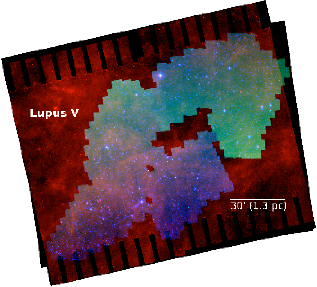
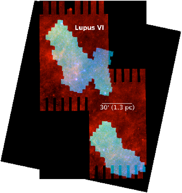
The Lupus V and Lupus VI dark clouds were observed using the Spitzer Space Telescope IRAC and MIPS cameras at 3.6, 4.5, 5.8, 8.0, 24 and 70 $\mu$ m on 1-8 April and 9 September 2007 as part of the Spitzer GB survey (PI: Lori E. Allen). A 3.82 deg² and 2.88 deg² areas were mapped in Lupus V and Lupus VI, respectively, covering entirely the cloud area where the visual extinction is greater than A ${}_{V}\approx$ 2 (Figure 1 and 2) in the extinction map reported by Cambrésy (1999). The observations in Lupus V and VI were performed to match the detection and sensitivity limits of the Spitzer c2d survey in Lupus I, III and VI.

Refer to caption — Figure 1: Color-composite image of the area in Lupus V mapped by the GB survey. North is up and East to the left. The color code is blue for the IRAC 2 band at 4.5 $\mu$ m, green for the IRAC 4 band at 8 $\mu$ m, and red for the MIPS 1 band at 24 $\mu$ m; note that the IRAC 2 and IRAC 4 mosaics cover exactly the same sky area. The figure shows the remnant cloud structure emitting at long wavelengths.

The data reduction procedure was essentially identical to the one used for all the c2d data. The IRAC and MIPS images were first processed by the Spitzer Science Center (SSC) using the standard pipeline to produce the Basic Calibrated Data (BCD). The c2d pipeline for IRAC data has been described by Harvey et al. (2006) and Jørgensen et al. (2006), while the pipeline for MIPS data has been described by Young et al. (2005) and Rebull et al. (2007). Using these BCD images, the final source catalogs were produced following four additional steps:

1.

Extra bad-pixel masking, image correction for muxbleed, column pull-downs/pull-ups as well as correction for the “first frame” effect in the third IRAC band (Harvey et al., 2006);
2.

Mosaicking of the individual frames. This was done with the SSC’s “Mopex” software suite (Makovoz & Marleau, 2005), which eliminates detector transient effects and transient sources (like asteroids) from the mosaics;
3.

Source location and extraction from the stacked mosaics, using the c2d developed tool c2dphot (Harvey et al., 2006). This software extracts photometry and calculates the uncertainties using digitized point spread functions. It also gives a morphological classification of the extracted sources (point-like or extended);
4.

Cross-identification of the sources among the 4 IRAC bands and merging of the final IRAC catalog with the MIPS 24 and 70 $\mu$ m catalogs (Chapman et al., 2007) and with the near-IR 2 $\mu$ m All Sky Survey (2MASS) catalog (Cutri et al., 2003). For the band merging, we used a 2.0^′′ match radius among IRAC bands and 2MASS and 4.0^′′ and 8.0^′′ for matching with MIPS bands 24 and 70 $\mu$ m, respectively, to account for the larger point spread functions of the MIPS bands.

For further information on the data reduction procedure we defer the reader to the delivery document by Evans et al. (2007). Table 1 summarizes the number of sources detected with signal-to-noise ratio of at least 5 in each band in the two surveyed areas in Lupus V and VI. Note that most of the detected objects are background giant or foreground dwarf stars at the brighter flux levels, while extragalactic objects make a substantial contribution to the fainter source counts.

3 Selection of YSO candidates

The main goal of the GB observations is the selection of YSO candidates based on their IR excess emission with respect to older field stars. However, the IR colors of many galaxies are very similar to those of YSOs. Thus, a sample of YSO candidates must be corrected for the contamination of background extragalactic objects. To distinguish YSOs from galaxies, we used a combination of 2MASS, IRAC and MIPS color-color (CC) and color-magnitude (CM) diagrams. This method has been developed within the frame of the Spitzer c2d Legacy Survey and has proven to be a success. Indeed, most of YSO candidates selected in Cha II, Lupus III and Serpens have been subsequently observed via spectroscopy and the YSO nature has been confirmed for $\sim$ 70% of them (see, e.g., Spezzi et al., 2008; Merín et al., 2008; Oliveira et al., 2009; Cieza et al., 2010).

A detailed review of the selection method can be found in Harvey et al. (2007a, b). Briefly, the selection method consists in the definition of an empirical probability function which depends on the relative position of a given source in several CC and CM diagrams, where diffuse boundaries have been determined to obtain an optimal separation between young stars and galaxies.

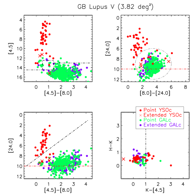
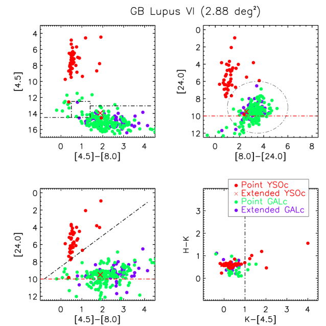
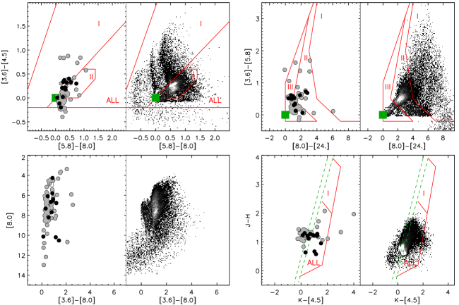
Figures 3 and 4 show the Spitzer CC and CM diagrams used to select the YSO candidates in Lupus V and VI, respectively. Note that the method requires detection in all IRAC bands and in MIPS1 with a S/N higher than 3 to classify an object as a YSO candidate or a background galaxy. Moreover, older field objects with no IR excess emission are rejected a priori because their IR colors are comparable with normal photospheric colors (e.g., $K-4.5<$ -0.1; Harvey et al., 2007a). We find 43 YSO candidates in Lupus V and 45 in Lupus VI, shown in Figures 3 and 4 as red dots and crosses for point-like and extended sources, respectively. All the YSO candidates have been visually inspected in the IRAC and MIPS images; they appear point-like in all our images and their photometry is not contaminated by crowding, nearby saturated stars or any other artifact that might affect our selection criterion. A remaining caveat is that our YSO candidates might be members of binary/multiple systems too close to be resolved with IRAC/MIPS and, hence, affecting the measured photometry. The multiplicity fraction for low mass stars (0.5-1 M_⊙) is estimated to be between 20% and 40%, depending on the actual mass of the primary star and the separation range (Duquennoy & Mayor, 1991; Mason et al., 1998; Basri & Reiners, 2006; Lada, 2006). Higher resolution photometry or spectroscopy would be needed to assess the actual multiplicity fraction in Lupus V and VI. The effect of multiplicity on the disk properties of YSOs are discussed in Sect. 5.2.

Interestingly, none of these 88 sources in Lupus V and VI was classified as a pre-main sequence star from previous ground-based optical/near-IR observations and none of them was detected by the ROSAT X-ray survey (Krautter et al., 1997) or by the IRAS satellite. This “non-detection/classification” is most likely due to photometric incompleteness and lack of dedicated observations for these two clouds. Indeed, no deep optical/near-IR surveys, comparable to those conducted in other Lupus clouds (Comerón et al., 2009), are available so far for Lupus V and VI. Prior to our Spitzer GB observations, only 5 far-IR sources were identified in these two clouds by the IRAS satellite (see Table 5 by Comerón, 2008). As for X-ray surveys, the ROSAT all sky survey detected about 200 weak-line T Tauri stars in the Lupus complex mainly concentrated around Lupus III (Krautter et al., 1997). Only an handful of them ( $\sim$ 10) are associated with Lupus V and VI, but none of these X-ray sources overlaps with our YSO candidates. No dedicated X-ray observations with XMM or Chandra have been conducted in these two clouds.

In Table 2-3 we list IRAC/MIPS fluxes of the YSO candidates selected in Lupus V and VI, while in Table 4-5 we report their 2MASS magnitudes.

4 Properties of the YSO candidates

4.1 Spectral Energy Distributions and IR Class

For each of the YSO candidates selected in Lupus V and VI we constructed the spectral energy distribution (SED), which can be used to constrain specific physical properties of the YSO population to be compared with those of other young populations observed with Spitzer. For all objects, the GB catalog provides the 2MASS near-IR magnitudes and the IRAC 3.6-8 $\mu$ m and MIPS 24-70 $\mu$ m fluxes. We complemented these data with optical photometry (BVRI) from the NOMAD (Zacharias et al., 2005) and DENIS (The, 2005) catalogs, thus obtaining complete SEDs from optical to infrared wavelengths depending on available data. Figures 5-8 show the SEDs for all YSO candidates in Lupus V and Lupus VI. In each plot we also show, only for visual comparison purposes, the NextGen model spectrum corresponding to a K7 stellar photosphere (Hauschildt et al., 1999) normalized to the J-band dereddened flux. To perform this comparison, we roughly estimate the visual extinction toward each YSO candidate by fitting the observed photometry between V and J with the NextGen model spectrum, arbitrarily assuming a K7 spectral type and $\log g=$ 4, e.g. the typical values of T Tauri stars in Taurus (see Hartmann et al., 2005). The dereddened flux at each pass-band was obtained adopting the extinction law by Weingartner & Draine (2001) with $R_{V}$ =5.5, also adopted for other Lupus clouds (Merín et al., 2008). Each plot in Figures 5-8 also shows, for comparison, the typical SED of an optically thick accreting disk, i.e. the median SED of T Tauri stars in Taurus (D’Alessio et al., 1999) normalized to the dereddened J-band flux. From these comparisons, it is clear that the SEDs of our YSO candidates show considerable variety. An ideal classification system has to rely on disk models, which are degenerate in several parameters (Robitaille et al., 2007), and also requires a good knowledge of the physical parameters of the central star (spectral type, reddening, etc), which are not available from the literature for our YSO candidate sample. Therefore, we do not attempt a full disk characterization of each SED but rather classify our objects on the basis of several SED slopes, following the approach adopted in other c2d/GB papers (Harvey et al., 2007a; Merín et al., 2008; Alcalá et al., 2008).

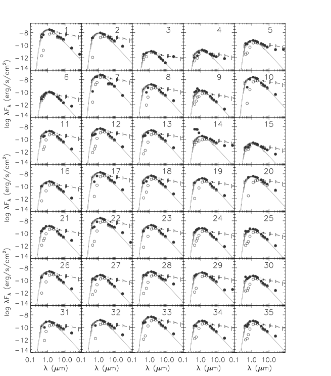
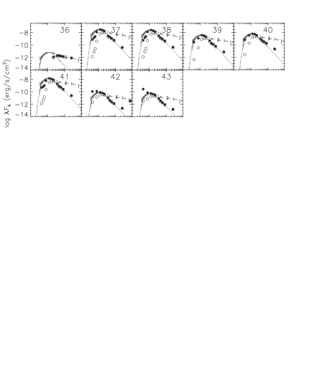
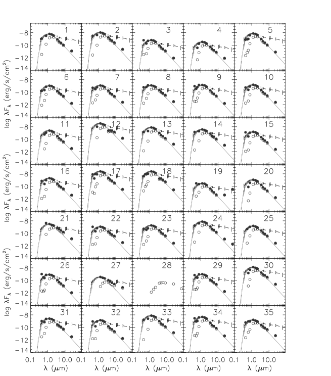
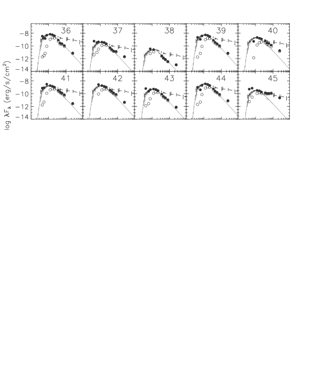
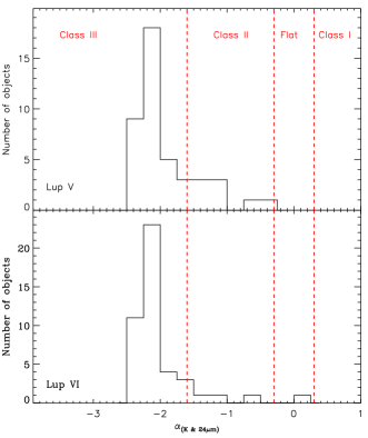
We grouped the YSO candidates identified in Lupus V and VI in four IR classes (Class I, Flat, Class II and Class III) following the scheme proposed by Lada & Wilking (1984) and Greene et al. (1994). Such grouping allows distinguishing between stars with optically thick and optically thin disks¹¹1In this paper we use the definition “optically thin disk” to indicate a disk optically thin at most radii to the radiation from the star. This kind of disk is usually associated with a disk-to-stellar luminosity ratio of $L_{disk}/L_{star}<$ 0.01 (Evans et al., 2009b).; overall, such classification gives a good overview of the evolutionary state of YSOs within a cloud. This classification uses the spectral slope ( $\alpha$ ) of the SED at wavelengths longer than 2 $\mu$ m; in our case, we computed the spectral slope of each SED by performing a least squares fit of all available data in the K-24 $\mu$ m range and divided our sample in the four classes according to the following criteria: Class I $\Rightarrow$ $\alpha\geq$ 0.3, Flat $\Rightarrow$ -0.3 $\leq\alpha<$ 0.3, Class II $\Rightarrow$ -1.6 $\leq\alpha<$ -0.3, Class III $\Rightarrow$ $\alpha<$ -1.6. The values of $\alpha$ -slope for the YSO candidates Lupus V and VI are reported in Table 6 and 7. Figure 9 shows the distribution of spectral slopes for both clouds and Table 8 lists the number of sources in each of the four classes. From Table 8 and Figure 9 we can immediately see that both clouds contain a high fraction of Class III objects (79% for Lupus V and 87% for Lupus VI), while all other clouds observed with Spitzer show a higher abundance of Class II objects (see Sect. 5). We confirm this classification based on the computation of a single slope ( $\alpha$ ) by applying several alternative methods, which are described in Appendix A. We also stress that the percentages we estimate are lower limits to the actual number of Class III sources in Lupus V and VI, since our selection criteria require a mid-IR excess and, hence, not all Class III sources are recovered, having them in many cases normal stellar photospheric colors. Indeed, X-ray observations of Cr A revealed a significant larger number of Class III objects in this cloud than selected by the Spitzer GB survey (Peterson et al., submitted).

4.2 Interesting objects

4.2.1 Transition objects

Transition disks represent a critical benchmark for disk evolution and planet formation models and it is therefore crucial to study their properties on a statistically significant basis.

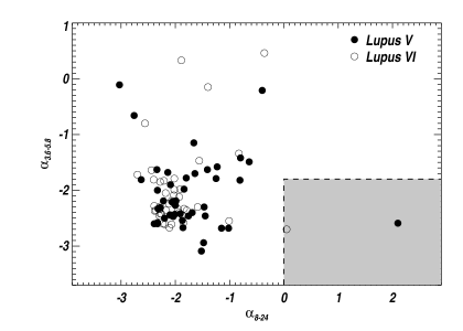
We searched for possible transition objects among the YSO candidates identified in both Lupus V and VI. We used the method proposed by Muzerolle et al. (2010) and plot the SED slope in the 3.6-5.8 $\mu$ m interval ( $\alpha_{3.6-5.8}$ ) versus the SED slope in the 8-24 $\mu$ m interval ( $\alpha_{8-24}$ ). These slope values are reported in Table 6 and 7. Figure 10 shows the $\alpha_{3.6-5.8}$ versus $\alpha_{8-24}$ diagram and the dotted lines define the region where transition objects are expected ( $\alpha_{8-24}>$ 0 and $\alpha_{3.6-5.8}<$ -1.8). We find two potential transition objects, namely ID 3 in Lupus V and ID 19 in Lupus VI, which are marked with an asterisk in Table 6-7. The transitional nature of these two objects is also supported on the basis of other SED parameters indicating the presence of a inner hole in their disks (see Sect. A.3 and Figure 19).

4.2.2 Flat sources

Flat-spectrum sources, whose emission arises from both a disk and an envelope likely possessing a wind-carved cavity (Greene et al., 1994; Evans et al., 2009b), are believed to be the boundary between protostars and pre-main sequence objects. This phase is one of the most interesting in the evolution of YSOs as phenomena such as outflows and mass accretion, which determine the final mass of the star and process the surrounding material, are particularly active.

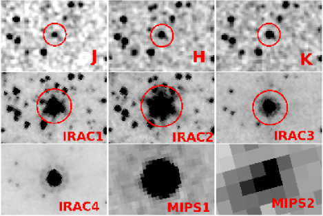
The YSO candidates sample selected in Lupus V and VI contains only one flat sources, namely ID 28 in Lupus VI, and its SED in shown in Figure 7. This object in not detected at optical wavelength neither by the NOMAD nor by the DENIS surveys, as expected for young objects still partially embedded, and appears point-like in all the 2MASS and Spitzer 3.6-24 $\mu$ m images (Figure 11). This source was recently observed, and not detected, in the HCO⁺(3-2) sub-millimeter line by Amanda Heiderman (private communication) using the 10m Caltech Submillimeter Observatory (CSO) in Mauna Kea (Hawaii). van Kempen et al. (2009) presented a YSO classification method based on HCO $+$ lines that successfully separates embedded Class I sources (strong HCO $+$ emission) from edge-on Class II disks and confused sources (little or no HCO $+$ emission). The lack of detection in the HCO⁺(3-2) line casts doubt on the existence of a residual dense envelope around our flat-spectrum YSO candidate. The upper limit to its main beam HCO $+$ line temperature, computed as 2 $\sigma_{rms}$ , is $<$ 0.48 K.

4.3 Spatial distribution and clustering of the YSO candidates

The spatial distribution of YSOs in relation to the cloud structure can be used to study a very specific aspect of the star formation process, i.e. whether it occurs in a centrally condensed way or there is more than one center of density (see Lada & Lada, 2003, and references therein).

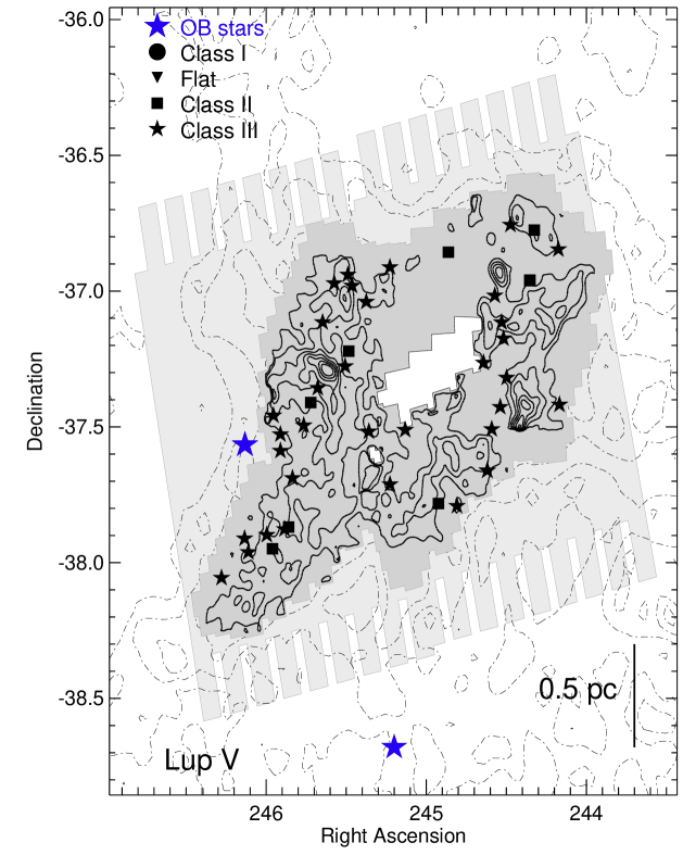
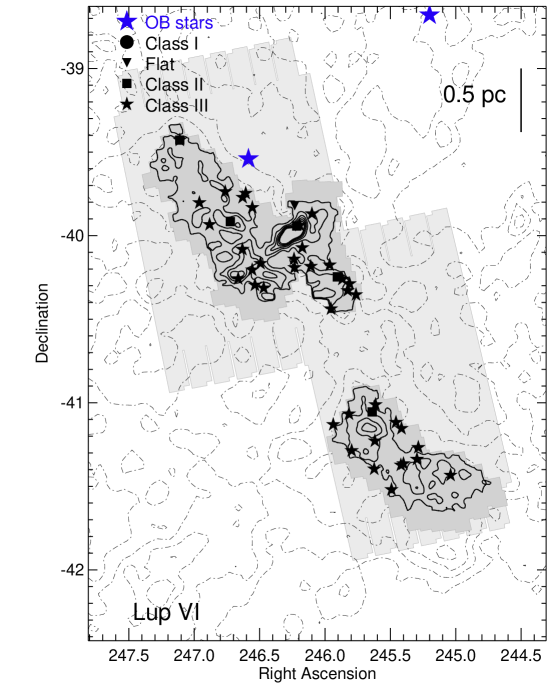
Figures 12 and 13 show the spatial distribution of the YSO candidates in the Lupus V and VI clouds on the relative extinction maps obtained from the Spitzer GB data. These extinction maps have a spatial resolution of 120 arcsec and the details on how such maps were derived are given in the final c2d data delivery document (Evans et al., 2007). In both clouds, the regions of high extinction (A ${}_{V}\gtrsim$ 6 mag) are rare. The great majority of the YSO candidates (of any SED class) lie in the vicinity of the highest extinction regions, however their position does not correlate with the location of the extinction peaks. A possible explanation is that star formation may have not taken place in these clouds very recently (i.e. more than 5-10 Myrs ago), so that their YSO populations appear now to be dispersed in the surroundings of the extinction peaks. This interpretation would fit with the high abundance of Class III objects in both clouds, but needs to be confirmed by velocity dispersion and age measurements (see Sect. 5).

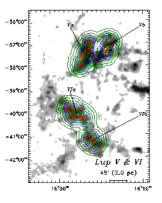
To investigate quantitatively the clustering properties of the YSOs candidates in Lupus V and VI, we applied Casertano & Hut (1985) surface/volume density algorithm, following the same approach as for the c2d clouds (see, e.g., Evans et al., 2009a). In particular, the criterion we adopt to identify YSO structures is described in detail by Jørgensen et al. (2008) and divides concentrations of YSOs into “clusters” or “groups”. “Clusters” are defined as regions with more than 35 YSOs within a given volume density level and ”groups” as regions with less. Clusters and groups can be “loose”, if their volume density is higher than 1 M ${}_{\odot}/pc^{3}$ , or ”tight” if their volume density is higher than 25 M ${}_{\odot}/pc^{3}$ . Figure 14 shows the result of the clustering analysis for Lupus V and VI. The YSO density contours are plotted, for comparison, on the extinction map. The YSO candidates are divided up into 4 loose groups, two in each cloud. While the two groups observed in Lupus V are definitively real, the discontinuous coverage of the IRAC observations in Lupus VI might have biased the algorithm result toward the identification of two separate YSO groups in this cloud. Furthermore, there are some low A_V clumps in the eastern part of the region with no associated YSO candidates; this is simply due to the fact that our Spitzer observations did not cover this part of the sky. Table 9 summarizes the results of the clustering analysis in Lupus V and VI; we report the number of YSO candidates, their Lada class, the cloud mass, the volume and the star formation efficiency (SFE) measured in each of the four loose groups. The cloud mass (M_cloud) was determined from the GB extinction map, while the SFE is defined as $M_{stars}/(M_{stars}+M_{cloud})$ , where the total mass converted into stars (M_stars) was estimated assuming an average YSO mass of 0.5 M_⊙, to be consistent with the estimates in Table 12 by Merín et al. (2008) for the other Lupus clouds, which we use for comparison. However, as we will see in Sect. 5.5, the YSO population in Lupus V and VI might have a characteristic stellar mass between 0.6 and 1.3 $M_{\odot}$ depending on the assumed age, higher than the other Lupus cloud and slightly higher than the peak of the standard IMF (e.g., Miller & Scalo, 1979; Chabrier, 2001; Kroupa & Weidner, 2005). Thus, in Table 9 we also include SFE calculations assuming the standard form of the IMF by Kroupa & Weidner (2005).

Lupus V and VI clearly show multiple density structures with separate gas concentrations that evolve independently and a SFE around 3-4% (assuming 0.5 M_⊙ as the typical YSO mass), similar to the SFE measured by Merín et al. (2008) for Lupus I and IV but lower than the SFE measured for Lupus III (see their Table 12). Overall, both the cloud density structure and the distribution of YSO candidates in the two regions suggest a dispersed distribution of volume density enhancements rather than a centrally-condensed structure. This dispersed distribution of YSOs, with peak densities of 2-4 YSO candidates per pc³ following the lane of the dust emission, is typical of Lupus I and IV, while in the more active Lupus III a centrally-condensed structure appears to dominate the star-formation process (Merín et al., 2008). In particular, the clustering analysis shows that the spatial distribution of Class III objects in Lupus V and VI is similar to that of Class III members in Lupus I and IV, while it is clearly more spread than the Class III population in Lupus III. This larger spread might indicate that the Lupus I and IV population is a few Myrs older than the Lupus III population, but again this hypothesis needs to be confirmed by velocity dispersion and age measurements. As we will see Sect. 5, a few Myrs older age (5-10 Myrs) for the stellar population in Lupus V and VI with respect to Lupus III would explain both the higher spatial dispersion and the higher fraction of Class III objects in these two clouds. Considering this age and given that the YSO candidates in Lupus V and VI are approximately dispersed over a 4 pc radius in both clouds (Figure 14), we expect their velocity dispersion to be of the order of 0.4-0.8 km/sec, which well matches the range observed for other galactic star forming regions and young clusters (see, e.g., Kraus & Hillenbrand, 2008, and reference therein).

5 Discussion

In the previous section we have shown that most YSO candidates in Lupus V (79 $\%$ ) and Lupus VI (87 $\%$ ) are surrounded by optically thin disks (Class III objects). To place our results in a more global context, we report in Table 8 the number of YSO candidates organized by IR class for all the Lupus clouds observed with Spitzer (Lupus I, III, IV, V, and VI; this work and Merín et al., 2008) and the other clouds observed with Spitzer within the frame of the c2d survey, namely Cha II (Alcalá et al., 2008), Perseus (Lai et al., in preparation), Serpens (Harvey et al., 2007b), and Ophiuchus (Allen et al., in preparation). We find a much higher number of the Class III objects in both Lupus V and Lupus VI than in Lupus I, III and IV. The difference gets even stronger when compared to the fraction of Class III objects measured in the c2d cloud sample and summarized in Evans et al. (2009a). To explain the origin of the surprisingly high fraction of Class III objects in Lupus V and Lupus VI, we considered the following possible scenarios and investigate them in more details in Sect. 5.1-5.5:

1.

Contamination: Contamination by field objects with small IR excess emission can affect the measured fraction of Class III YSO candidates.
2.

Binarity: Most circum-binary disks are cleared by ages of 1-2 Myr, while most circumstellar disks are not (Bouwman et al., 2006). Thus, a significantly higher fraction of binary stars in Lupus V and VI with respect to the other Lupus clouds would explain the higher fraction of Class III sources.
3.

Stellar age: Because Class II objects are very common at ages $\sim$ 1 Myr and very rare at $\sim$ 10 Myr (Sect. 1), a few Myrs older age for the stellar population in Lupus V and VI with respect to the other Lupus clouds (1.5-4 Myr; Hughes et al., 1994; Comerón et al., 2003) would also explain the higher fraction of Class III objects.
4.

Disk photo-evaporation: This scenario would rely on the presence of OB stars lying close enough to the Lupus V and VI YSO populations to photoevaporate their disks, but too far from the Lupus I, III and IV populations to have any influence on the evolution of their disks.
5.

Characteristic stellar mass: Recent studies suggest a much shorter disk dissipation time (Brown et al., 2007; Kim et al., 2009; Merín et al., 2010) and higher mass accretion rate for higher mass stars (Natta et al., 2004, 2006; Sicilia-Aguilar et al., 2006). Thus, a possible difference between the characteristic stellar mass in Lupus V and VI and the other Lupus clouds may be the cause of the different evolutionary stages of the observed disks.

Using our dataset and complementary information from the literature we now investigate these scenarios.

5.1 Contamination

The immediate explanation would be that our YSO candidates sample is significantly contaminated by field objects with small IR excess emission similar to that of Class III YSOs. The adopted YSO selection method has proven to be successful since most YSOs selected in the c2d clouds have been confirmed via spectroscopy (Spezzi et al., 2008; Merín et al., 2008; Oliveira et al., 2009; Cieza et al., 2010). The removal of extra-galactic objects is optimal and the fraction of contaminants, mainly consisting of AGB stars with small excess emission in IRAC and/or MIPS 24 $\mu$ m mimicking the behavior of Class III YSOs, is estimated to be around 30% (e.g. Oliveira et al., 2009; Cieza et al., 2010). This estimate is based on the spectroscopic follow-up of Class III objects in the Serpens molecular cloud, which is located at b $\approx+$ 5 deg from the galactic plane. Thus, we expect the higher galactic latitude of Lupus V and VI (6 $<b<$ 8 deg) to minimize this problem. However, even taking a 30% contamination level into account, the fraction of Class III YSO candidates in Lupus V and IV would reduce to 70% and 81%, respectively, and is still much higher than measured in other c2d clouds.

To verify further the amount of expected contamination, we have also estimated the numbers of background AGB stars expected towards the direction of Lupus V and VI over the areas observed with Spitzer. We performed this exercise by using the Galaxy model by Robin et al. (2003) and their online tool²²2http://model.obs-besancon.fr/. According to this model, we expect less than 1 background AGB stars in the 3.82 and 2.88 deg² areas observed in Lupus V and VI, respectively, with apparent $J$ magnitude between 5 and 16.5, i.e. the photometric ranges covered by our YSO candidates (Tables 4 and 5). Galactic counts models become more and more inaccurate towards the very low-mass regime and the predicted number depends on the adopted model, however this exercise ensures that AGB stars can not contribute noticeably to the contamination of our Class III YSO candidates.

5.2 Binarity

It has been shown that interactions with close stellar or planetary companions can significantly influence the evolution and lifetime of protoplanetary disks (Monin et al., 2007). In particular, Kraus & Ireland (2010) have shown that disk evolution of close (5-30 AU) binary systems is very different from that of single stars, and most circum-binary disks are cleared by ages of 1-2 Myrs, while most circumstellar disks around single stars are not (Bouwman et al., 2006). Thus, a significantly higher fraction of binary stars in Lupus V and VI with respect to the other Lupus cloud would also explain the high fraction of Class III sources. Specifically, the fraction of binary stars in Lupus V and VI should be about 50% higher than in the other Lupus clouds to account for the relative abundance of Class III YSOs.

There are no indications in the literature of a higher binary fraction in Lupus V and VI relative to other Lupus clouds and, hence, this scenario appears unlikely. However, we cannot definitively rule it out. High resolution spectroscopy (see, e.g., Prato, 2007) and/or adaptive optics and long-baseline interferometry would be necessary to properly measure the binary fraction in these clouds (e.g., Raghavan et al., 2007).

5.3 Stellar age

IR studies of individual star-forming regions have long suggested that disk lifetimes are relatively short ( $\lesssim$ 5 Myrs; Strom et al., 1989; Skrutskie et al., 1990; Lada & Lada, 1995; Brandner et al., 2000). Haisch et al. (2001) were the first to provide more precise constraints. They showed that the fraction of stars with disk within a cluster rapidly decreases with age, such that one-half the stars lose their disks within the first 3 Myr, and derived an overall disk lifetime of $\sim$ 6 Myr. More recently, Evans et al. (2009a) derived half-life for each of the Lada classes from the combined analysis of the Spitzer c2d dataset. According to this study, the half-life for Class II sources is $\sim$ 2 Myrs. Thus, an age of $\sim$ 10 Myr for the young population in Lupus V and VI, i.e. only a few Myrs older than the other Lupus clouds (1.5-4 Myr; Hughes et al., 1994; Comerón et al., 2003), would explain the higher fraction of Class III objects in these clouds.

We can not assess the presence of age differences of the order of a few Myrs among the Lupus clouds on the basis of the Spitzer and complementary data available at the moment in the literature. Optical photometry and spectroscopy would help to estimate isochronal ages and/or ages based on the LiI 670.8nm line for the YSO population in each Lupus cloud. However, these methods provide only weak constraints on the age (see, i.e., Palla et al., 2005), so that a possible age difference of a few Myrs between the Lupus V and VI population and the population in other Lupus clouds would not be clearly reflected by their LiI 670.8nm absorption line or position in optical/near-IR color magnitude diagrams. Moreover, the reliability of lithium abundance as an age indicator is even more limited after the recent finding that events of episodic accretion enhance the lithium depletion of low-mass stars and brown dwarfs (Baraffe & Chabrier, 2010). As for the isochronal age, the uncertainty on the distance to the Lupus clouds prevents a reliable derivation of the age based on the position of the objects in the temperature-luminosity diagram. This problem will be solved in the near future thanks to the forthcoming GAIA mission.

Beside the impossibility to put accurate constraints to the age of Lupus V and VI on the basis of Spitzer data, it is plausible that in these two clouds star formation ceased almost entirely a few Myrs ago while this is not the case for other Lupus clouds. Heiderman et al. (2010) investigate the relation between star formation rate (SFR) and gas surface densities ( $\Sigma_{gas}$ ) for 20 large molecular clouds from the c2d and GB surveys. This study revealed that the SFR surface density ( $\Sigma_{\rm SFR_{\rm IR}}$ ) versus $\Sigma_{gas}$ relation is a power law whose slope changes from a steep relation at $\Sigma_{gas}<\Sigma_{th}$ (slope of $\sim$ 4.6) to a linear relation (slope of $\sim$ 1.1) above $\Sigma_{th}$ . The authors estimate $\Sigma_{th}=$ 129 $\pm$ 14 M ${}_{\odot}/pc^{2}$ , corresponding to A ${}_{V}\approx$ 8.6 mag, and denote this as a star formation threshold. This does not imply no star formation below the threshold, but clearly indicates that the probability to find star forming cores is higher above the threshold. The star-forming threshold found by Heiderman et al. (2010) is in agreement with the threshold (A ${}_{V}\approx$ 7-10 mag) found in other studies of local molecular clouds (Onishi et al., 1998; Johnstone et al., 2004; Enoch et al., 2007; Lada et al., 2010; André et al., 2010). In other words, if most of the present-day mass measured for a given cloud lies below A ${}_{V}\approx$ 8 mag, a decrease in star formation could plausibly be caused by exhaustion of gas above such a threshold in surface density. In Table 10 we report the fraction of cloud mass below the threshold for Lupus V and VI and compare it with the fraction measured for the other Lupus clouds, in particular for Lupus III which is the most active star forming cloud in the complex and is mainly populated by Class II objects (see Table 8). It is clear that the cloud mass above threshold in Lupus V and VI is very small or zero, while in Lupus III and in the other Lupus clouds a significant fraction of the cloud mass is still above threshold. Thus, it is not surprising that star formation is still ongoing in Lupus III, as reflected by the substantial number of objects in younger SED classes. In contrast, the absence of such sources in Lupus V and VI could be explained by a cessation of active star formation a few Myrs ago. It may be hard to get an actual age difference between Lupus V and VI on the one hand and the other Lupus clouds on the other, both for the reasons mentioned above and because the oldest stars in each cloud may have similar ages. Table 10 only indicates that the duration of the star-forming event in Lupus V and VI was less because it started with less dense gas and used it up longer ago.

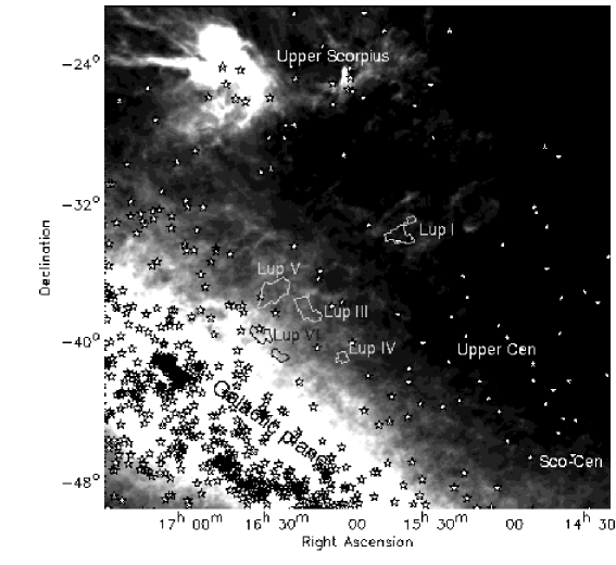
Another argument in favor of an older age of Lupus V and VI with respect to other Lupus clouds comes from their spatial location with respect to the Sco-Cen association. Lupus I, III, IV are all at high galactic latitude( $b\approx$ +9, +16 and +48, respectively), in the region of the Lupus complex closest to Sco-Cen (see Figure 15 and Figure 2 by Tachihara et al., 2001). In particular, Lupus I is at the edge of an HI shell left over from a supernova event in the Upper-Sco sub-group of Sco-Cen about 1.5 Myr ago (Tachihara et al., 2001). The dynamics of the HI and the CO towards Lupus I are consistent with the molecular cloud being compressed by the HI shell (Tothill et al., 2009), and this may have caused recent/ongoing star formation. Lupus III and IV lie in “streamers” that stretch from the main body of Lupus towards the Upper-Cen-Lup sub-group of Sco-Cen, but may also be exposed to effects from Upper-Sco. Thus, even though Lupus III and IV do not fit the argument so well as Lupus I, recent triggered star-formation might play a role in their star formation history, whereas Lupus V and VI lie at lower galactic latitudes ( $b\approx$ +8 and +6, respectively) and do not show any morphological evidence of interaction with Sco-Cen.

5.4 OB stars and disk photoevaporation

Circumstellar disks in stellar aggregates can be effectively evaporated within a few Myrs through the action of external ultraviolet radiation from the most massive stars in the group. The intensity and spatial extent of such radiation fields depends on the number and spectral type of the massive stars. For small groups of 100/500 members, which is the case of the Lupus complex, photoevaporation of disks around low-mass stars (M $\lesssim$ 1 M_⊙) is expected to be efficient within about 0.5-1 pc of the massive stars (see Johnstone et al., 1998; Störzer & Hollenbach, 1999; Adams et al., 2004; Balog et al., 2007; Guarcello et al., 2009, and references therein). Indeed, it has been recently shown that in the young open clusters NGC 2244 and NGC 6611, both containing a rich low-mass PMS population as well as a large number of OB stars, the disk frequency drops within a distance of $\sim$ 0.5 pc from the massive star group (Balog et al., 2007; Guarcello et al., 2009). At larger distances, however, stars with disks do not appear affected by the presence of massive stars, since the disk frequency is not spatially correlated with the positions of massive stars. We can consequently assume that any disk photoevaporation effect is expected to be seen within $\sim$ 1 pc from the ionizing OB stars.

We used the OB star catalog provided by C. Reed (Reed, 2003) and searched for OB stars lying in the vicinity, i.e. within 1 pc, of the Lupus clouds. Figure 15 shows the spatial distribution of massive OB stars together with the areas observed by Spitzer in Lupus I, III, IV, V and V as part of the c2d and GB surveys. In Table 11 we report the number of OB stars within 1 pc of each of the Lupus clouds, their spectral type and luminosity and the projected distance from the cloud. Because of the paucity of OB stars in the vicinity each cloud, it is very unlikely that photoevaporation plays a relevant role in the disk evolution of the YSOs in these clouds. In particular, for Lupus V and VI we found just one star lying within 1 pc from each cloud, as shown in more detail in Figure 12 and Figure 13, and this number is comparable to that found in Lupus I, III and IV. Thus, there is no evidence that disk photoevaporation is acting more efficiently in Lupus V and VI then in the other Lupus clouds. Moreover, both for Lupus V and VI, we did not find any spatial correlation between the Class II disk frequencies and the position of these massive stars. For instance, in Lupus VI, Class II YSO candidates are more abundant within 1 pc from the only B-type star in the field than further away. Another argument discharging the photoevaporation hypothesis is that the radius up to which a star can externally photoevaporate a disk depends on the square root of its ionizing flux, which in turn depends on the spectral type (see, e.g., Johnstone et al., 1998; Störzer & Hollenbach, 1999; Adams et al., 2004; Balog et al., 2007; Guarcello et al., 2009). Radii of the order of 0.5-1 pc apply to early and mid-type O stars, which have ionizing fluxes orders of magnitude greater than those of mid or late B stars. As Table 11 indicates, the nearest stars to the Lupus clouds have mid or late B types, and are thus virtually harmless to any nearby disks.

For these overall reasons, it is very unlikely that the proximity of massive stars could be the cause of the high abundance of Class III YSO candidates in Lupus V and VI.

5.5 Luminosity function and characteristic stellar mass

The determination of the stellar luminosity can be used as a poor but still useful first order proxy for mass, assuming that most of the stars have formed more or less at the same time. Before using the range of luminosities to provide an estimate of the mass range, we determined the degree of completeness of the YSO candidate sample in Lupus V and VI. We used the same approach as Merín et al. (2008) and derive first the bolometric luminosity function for Lupus V and VI. The bolometric luminosity of each YSO candidate was obtained by integrating over the entire observed SED flux; the total flux was finally converted to luminosity assuming a distance of 150 pc for both Lupus V and VI clouds (Comerón et al., 2009). We then applied Harvey et al. (2007b)’s completeness estimate for the c2d survey to our YSO candidate samples, since the GB catalogs have the same photometric depth as the c2d ones. Harvey et al. (2007b) made an estimate of the completeness of the c2d catalogs by comparing, for each luminosity bin, the number of counts from a trimmed version of the deeper SWIRE catalog of extragalactic sources (assumed to represent 100 $\%$ completeness by c2d standards) with the number of counts for the c2d catalogs in Serpens. This completeness estimate has been applied to all five molecular clouds observed within the c2d frame, under the assumption that the Spitzer observations for these clouds were homogeneous in terms of photometric depth. Figure 16 shows the bolometric luminosity function for Lupus V and VI before (solid line) and after (dashed line) correction for completeness and suggests that we are missing only a few low-luminosity objects with $L<0.1L_{\odot}$ , i.e. $\sim$ 4 in Lupus V and $\sim$ 1 in Lupus VI. These objects have been missed by our selection either because they are below the noise level of our GB observations or because they are located within the galaxy loci of the CM diagrams (Figure 3-3). In conclusion, both luminosity histograms suggest a completeness better than $\sim$ 85% at luminosities down to 0.1 L_⊙ for the YSO candidate samples in Lupus V and VI, which corresponds to a mass of 0.1, 0.2 and 0.35 M_⊙ for 1, 5 and 10 Myrs old stars, respectively, according to the PMS evolutionary tracks by Baraffe et al. (1998).

Both Lupus V and VI clouds the peak of the luminosity function appears between 0.5 and 0.6 L_⊙, which corresponds to a 0.6 M_⊙ star at an age of 1 Myr and to a 1.3 M_⊙ star at an age of 5 Myr. Note that most young stars within the Lupus complex have an estimated age which falls within the 1-5 Myr interval (Comerón, 2008). The bolometric luminosity histogram for the other Lupus clouds (see Figure 13 by Merín et al., 2008) suggests a typical luminosity of 0.2 $L_{\odot}$ , which corresponds to a 0.2 M_⊙ star at an age of 1 Myr and to a 1 M_⊙ star at an age of 5 Myrs. Thus, YSO candidates in Lupus V and VI are on the average 0.4 M_⊙ more massive than YSOs in the other Lupus clouds. As mentioned in Sect. 5, this difference may have some impact on the observed properties of disks because the disk lifetime and mass accretion rate both appear to depend on stellar mass (Brown et al., 2007; Kim et al., 2009; Merín et al., 2010; Muzerolle et al., 2010; Sicilia-Aguilar et al., 2010). Because of the large uncertainties and limitations affecting the measurement of both the disk lifetime and the mass accretion rate, it is still very premature to give a disk lifetime versus stellar mass calibration relation and, hence, estimate whether a 0.4 M_⊙ difference in the characteristic stellar mass is significant. Moreover, the Lupus complex extends over about 50 pc along the line of sight (see Sect. 3 by Comerón et al., 2009). Thus, the difference in the characteristic stellar mass we measure among the Lupus clouds might be partly due to the use of inaccurate distances for each individual cloud. However, the incorrect distance can hardly be the only cause of the greater peak in the luminosity function of Lupus V and VI, since bringing down the peak in luminosity (and therefore in mass) by a factor of $\sim$ 3 would require these clouds to be at $\sim$ 70% of the assumed distance, placing them at 100 pc or less from the Sun, which seems unlikely.

Thus, it is worth mentioning that the higher characteristic stellar mass of Lupus V and VI might be a contributing factor to the high fraction of Class III YSO candidates observed in these clouds.

Table 1: Lupus V and VI detection statistics.

	Lupus V	Lupus VI
Detection criterion	Number of sources
IRAC 3.6 $\mu$ m with S/N $\geq$ 5	292611	243185
IRAC 4.5 $\mu$ m with S/N $\geq$ 5	179095	168863
IRAC 5.8 $\mu$ m with S/N $\geq$ 5	33870	32436
IRAC 8.0 $\mu$ m with S/N $\geq$ 5	18366	17548
All 4 IRAC bands with S/N $\geq$ 5	14571	13632
MIPS 24 $\mu$ m with S/N $\geq$ 5	1816	2469
MIPS 70 $\mu$ m with S/N $\geq$ 5	126	87
All 4 IRAC bands, MIPS 24 $\mu$ m, & K with S/N $\geq$ 5	558	526

Table 2: IRAC and MIPS observed fluxes for the YSO candidates in Lupus V.

ID	Name/Position	3.6 $\mu$ m	4.5 $\mu$ m	5.8 $\mu$ m	8.0 $\mu$ m	24 $\mu$ m	70 $\mu$ m
	(SSTgbsJ)	(mJy)	(mJy)	(mJy)	(mJy)	(mJy)	(mJy)
1	16163197-3704563	2000.00 $\pm$ 169.00	2270.00 $\pm$ 132.00	2360.00 $\pm$ 113.00	1790.00 $\pm$ 90.80	259.00 $\pm$ 26.80	81.70 $\pm$ 10.20
2	16164035-3725054	1860.00 $\pm$ 109.00	1500.00 $\pm$ 80.90	1330.00 $\pm$ 64.70	1010.00 $\pm$ 48.20	499.00 $\pm$ 46.60	–
3	16164198-3650456	1.54 $\pm$ 0.08	1.03 $\pm$ 0.05	0.72 $\pm$ 0.05	0.41 $\pm$ 0.04	12.20 $\pm$ 1.17	–
4	16171811-3646307	4.64 $\pm$ 0.24	3.96 $\pm$ 0.19	3.67 $\pm$ 0.18	3.89 $\pm$ 0.20	5.78 $\pm$ 0.58	–
5	16172474-3657333	178.00 $\pm$ 8.60	167.00 $\pm$ 8.42	146.00 $\pm$ 6.91	122.00 $\pm$ 5.91	152.00 $\pm$ 14.10	468.00 $\pm$ 49.20
6	16172485-3657407	21.90 $\pm$ 1.04	14.30 $\pm$ 0.70	9.79 $\pm$ 0.47	5.58 $\pm$ 0.28	4.74 $\pm$ 1.17	–
7	16175383-3645207	2280.00 $\pm$ 293.00	3200.00 $\pm$ 221.00	3500.00 $\pm$ 167.00	2200.00 $\pm$ 119.00	237.00 $\pm$ 22.00	–
8	16175958-3719083	205.00 $\pm$ 10.10	120.00 $\pm$ 6.02	104.00 $\pm$ 4.91	72.40 $\pm$ 3.52	33.90 $\pm$ 3.16	–
9	16180425-3710277	21.20 $\pm$ 1.03	13.20 $\pm$ 0.63	9.84 $\pm$ 0.48	7.24 $\pm$ 0.34	1.58 $\pm$ 0.25	–
10	16180702-3706544	2460.00 $\pm$ 144.00	1780.00 $\pm$ 123.00	1590.00 $\pm$ 78.90	1090.00 $\pm$ 52.50	328.00 $\pm$ 30.60	–
11	16180915-3725364	248.00 $\pm$ 12.70	163.00 $\pm$ 10.00	132.00 $\pm$ 6.49	86.90 $\pm$ 4.16	21.30 $\pm$ 1.98	–
12	16181727-3700597	601.00 $\pm$ 30.10	345.00 $\pm$ 19.30	291.00 $\pm$ 14.30	176.00 $\pm$ 8.45	47.20 $\pm$ 4.38	–
13	16183414-3715488	344.00 $\pm$ 17.50	214.00 $\pm$ 11.00	193.00 $\pm$ 9.41	129.00 $\pm$ 6.09	33.60 $\pm$ 3.13	–
14	16191403-3747281	99.70 $\pm$ 5.00	85.60 $\pm$ 4.20	67.40 $\pm$ 3.29	59.20 $\pm$ 2.80	73.30 $\pm$ 6.78	241.00 $\pm$ 28.30
15	16192683-3651238	7.95 $\pm$ 0.38	6.98 $\pm$ 0.34	5.89 $\pm$ 0.28	5.24 $\pm$ 0.25	3.33 $\pm$ 0.37	–
16	16194163-3746568	85.60 $\pm$ 4.32	56.40 $\pm$ 2.73	47.70 $\pm$ 2.27	32.60 $\pm$ 1.56	10.20 $\pm$ 0.96	–
17	16203160-3730407	2070.00 $\pm$ 122.00	1240.00 $\pm$ 81.50	1270.00 $\pm$ 73.70	910.00 $\pm$ 56.50	211.00 $\pm$ 19.70	–
18	16205438-3742415	614.00 $\pm$ 31.90	399.00 $\pm$ 22.20	324.00 $\pm$ 16.10	200.00 $\pm$ 9.45	46.80 $\pm$ 4.34	–
19	16205449-3654430	224.00 $\pm$ 11.20	116.00 $\pm$ 5.69	99.70 $\pm$ 4.71	64.30 $\pm$ 3.03	25.10 $\pm$ 2.33	–
20	16212600-3731015	757.00 $\pm$ 40.90	529.00 $\pm$ 27.20	518.00 $\pm$ 26.00	387.00 $\pm$ 18.20	161.00 $\pm$ 14.90	–
21	16212991-3702213	189.00 $\pm$ 9.34	99.40 $\pm$ 4.80	83.70 $\pm$ 3.92	57.90 $\pm$ 2.73	56.90 $\pm$ 5.27	–
22	16215125-3658489	2190.00 $\pm$ 147.00	2100.00 $\pm$ 126.00	2040.00 $\pm$ 98.90	2020.00 $\pm$ 111.00	976.00 $\pm$ 91.40	83.10 $\pm$ 16.20
23	16215624-3713167	243.00 $\pm$ 12.40	131.00 $\pm$ 6.58	115.00 $\pm$ 5.47	73.80 $\pm$ 3.57	28.40 $\pm$ 2.64	–
24	16215748-3656219	81.90 $\pm$ 4.03	51.40 $\pm$ 2.44	38.30 $\pm$ 1.81	25.90 $\pm$ 1.21	5.99 $\pm$ 0.59	–
25	16220163-3716369	65.00 $\pm$ 3.16	42.30 $\pm$ 2.08	35.30 $\pm$ 1.67	24.80 $\pm$ 1.20	8.24 $\pm$ 0.79	–
26	16221789-3658165	342.00 $\pm$ 17.30	195.00 $\pm$ 9.72	168.00 $\pm$ 8.19	108.00 $\pm$ 5.13	34.40 $\pm$ 3.20	–
27	16223532-3706530	83.70 $\pm$ 4.10	47.30 $\pm$ 2.29	38.70 $\pm$ 1.82	24.00 $\pm$ 1.13	5.59 $\pm$ 0.55	–
28	16224265-3721232	361.00 $\pm$ 18.60	274.00 $\pm$ 13.90	247.00 $\pm$ 12.50	261.00 $\pm$ 13.00	198.00 $\pm$ 18.30	–
29	16225309-3724374	298.00 $\pm$ 14.80	234.00 $\pm$ 11.70	202.00 $\pm$ 9.70	135.00 $\pm$ 6.43	22.40 $\pm$ 2.09	81.00 $\pm$ 17.60
30	16230368-3729411	66.40 $\pm$ 3.19	41.70 $\pm$ 2.05	35.50 $\pm$ 1.67	31.20 $\pm$ 1.51	18.60 $\pm$ 1.73	–
31	16232050-3741193	183.00 $\pm$ 9.33	165.00 $\pm$ 7.97	139.00 $\pm$ 6.64	125.00 $\pm$ 6.00	97.60 $\pm$ 9.08	–
32	16232638-3752082	324.00 $\pm$ 16.50	247.00 $\pm$ 12.80	233.00 $\pm$ 11.80	174.00 $\pm$ 8.28	49.60 $\pm$ 4.61	–
33	16233246-3752361	568.00 $\pm$ 28.80	323.00 $\pm$ 16.60	285.00 $\pm$ 13.60	192.00 $\pm$ 9.13	70.90 $\pm$ 6.58	–
34	16233857-3735169	149.00 $\pm$ 7.42	95.90 $\pm$ 4.79	74.60 $\pm$ 3.53	50.00 $\pm$ 2.38	14.90 $\pm$ 1.39	–
35	16233865-3731388	143.00 $\pm$ 6.89	75.90 $\pm$ 3.74	70.50 $\pm$ 3.32	51.60 $\pm$ 2.44	31.40 $\pm$ 2.92	–
36	16234903-3727291	2.10 $\pm$ 0.10	2.67 $\pm$ 0.13	3.07 $\pm$ 0.15	3.36 $\pm$ 0.17	6.46 $\pm$ 0.67	–
37	16235052-3756560	2420.00 $\pm$ 175.00	2130.00 $\pm$ 98.60	1790.00 $\pm$ 88.80	1240.00 $\pm$ 63.20	284.00 $\pm$ 26.30	–
38	16235907-3753528	2510.00 $\pm$ 143.00	1610.00 $\pm$ 80.20	1410.00 $\pm$ 68.30	950.00 $\pm$ 45.00	319.00 $\pm$ 30.60	–
39	16242666-3757407	410.00 $\pm$ 20.80	214.00 $\pm$ 11.00	202.00 $\pm$ 9.78	129.00 $\pm$ 6.21	56.20 $\pm$ 5.21	–
40	16243230-3754398	855.00 $\pm$ 43.30	607.00 $\pm$ 30.00	533.00 $\pm$ 26.70	428.00 $\pm$ 20.30	170.00 $\pm$ 15.70	–
41	16250690-3803214	1640.00 $\pm$ 88.20	941.00 $\pm$ 50.50	820.00 $\pm$ 39.90	539.00 $\pm$ 25.90	178.00 $\pm$ 16.50	–
42	16182188-3730299	11.20 $\pm$ 0.91	5.57 $\pm$ 0.43	4.09 $\pm$ 0.28	3.05 $\pm$ 0.19	1.73 $\pm$ 0.31	73.30 $\pm$ 10.90
43	16182852-3739386	7.74 $\pm$ 0.56	4.28 $\pm$ 0.26	3.05 $\pm$ 0.19	2.00 $\pm$ 0.11	1.18 $\pm$ 0.24	–

Table 3: IRAC and MIPS observed fluxes for the YSO candidates in Lupus VI.

ID	Name/Position	3.6 $\mu$ m	4.5 $\mu$ m	5.8 $\mu$ m	8.0 $\mu$ m	24 $\mu$ m	70 $\mu$ m
	(SSTgbsJ)	(mJy)	(mJy)	(mJy)	(mJy)	(mJy)	(mJy)
1	16200205-4137264	727.00 $\pm$ 37.20	428.00 $\pm$ 22.70	360.00 $\pm$ 17.20	231.00 $\pm$ 10.90	90.00 $\pm$ 8.38	–
2	16200950-4126003	1400.00 $\pm$ 71.90	877.00 $\pm$ 47.00	788.00 $\pm$ 40.20	520.00 $\pm$ 25.00	161.00 $\pm$ 14.90	–
3	16210869-4116025	80.50 $\pm$ 3.96	50.40 $\pm$ 2.42	40.00 $\pm$ 1.88	28.10 $\pm$ 1.32	6.71 $\pm$ 0.65	–
4	16211125-4120172	47.60 $\pm$ 2.50	28.90 $\pm$ 1.38	23.80 $\pm$ 1.14	16.20 $\pm$ 0.77	6.17 $\pm$ 0.62	–
5	16213597-4121525	825.00 $\pm$ 43.40	455.00 $\pm$ 23.30	381.00 $\pm$ 18.60	234.00 $\pm$ 12.30	60.30 $\pm$ 5.58	–
6	16213962-4109135	141.00 $\pm$ 7.11	96.30 $\pm$ 4.76	76.00 $\pm$ 3.59	52.10 $\pm$ 2.45	12.80 $\pm$ 1.20	–
7	16214077-4122218	158.00 $\pm$ 7.92	86.30 $\pm$ 4.38	73.60 $\pm$ 3.45	48.60 $\pm$ 2.31	19.20 $\pm$ 1.79	–
8	16214973-4107017	192.00 $\pm$ 9.39	134.00 $\pm$ 6.60	108.00 $\pm$ 5.09	74.80 $\pm$ 3.59	24.00 $\pm$ 2.23	–
9	16215797-4131099	167.00 $\pm$ 8.46	103.00 $\pm$ 5.23	86.40 $\pm$ 4.09	55.70 $\pm$ 2.70	12.20 $\pm$ 1.14	–
10	16222724-4100410	198.00 $\pm$ 9.83	114.00 $\pm$ 5.62	91.30 $\pm$ 4.28	60.20 $\pm$ 2.84	18.60 $\pm$ 1.73	–
11	16222844-4113424	252.00 $\pm$ 12.90	149.00 $\pm$ 7.15	125.00 $\pm$ 5.95	80.60 $\pm$ 3.82	24.60 $\pm$ 2.28	–
12	16222966-4123457	1840.00 $\pm$ 206.00	2670.00 $\pm$ 168.00	3480.00 $\pm$ 220.00	2820.00 $\pm$ 136.00	1060.00 $\pm$ 101.00	–
13	16223341-4103179	822.00 $\pm$ 45.10	495.00 $\pm$ 25.00	426.00 $\pm$ 20.40	287.00 $\pm$ 13.60	121.00 $\pm$ 11.20	–
14	16230307-4021119	651.00 $\pm$ 40.60	379.00 $\pm$ 20.10	377.00 $\pm$ 20.10	231.00 $\pm$ 11.10	82.70 $\pm$ 7.68	–
15	16231101-4117103	167.00 $\pm$ 8.61	115.00 $\pm$ 5.88	92.10 $\pm$ 4.35	61.60 $\pm$ 2.92	17.90 $\pm$ 1.67	–
16	16231476-4017151	220.00 $\pm$ 11.70	136.00 $\pm$ 6.71	115.00 $\pm$ 5.56	81.50 $\pm$ 3.89	28.60 $\pm$ 2.67	–
17	16231598-4104009	1800.00 $\pm$ 126.00	1310.00 $\pm$ 70.60	1120.00 $\pm$ 55.30	736.00 $\pm$ 35.40	241.00 $\pm$ 22.50	–
18	16231844-4019439	1490.00 $\pm$ 147.00	2080.00 $\pm$ 107.00	1660.00 $\pm$ 87.60	1170.00 $\pm$ 55.30	210.00 $\pm$ 19.50	–
19	16232809-4015368	37.70 $\pm$ 1.87	22.80 $\pm$ 1.09	16.70 $\pm$ 0.87	9.83 $\pm$ 0.47	31.10 $\pm$ 2.90	771.00 $\pm$ 81.10
20	16233735-4014490	136.00 $\pm$ 6.91	70.80 $\pm$ 3.64	60.50 $\pm$ 2.93	38.50 $\pm$ 1.82	11.40 $\pm$ 1.07	–
21	16234486-4107493	595.00 $\pm$ 31.30	470.00 $\pm$ 27.30	407.00 $\pm$ 20.20	302.00 $\pm$ 15.40	98.80 $\pm$ 9.16	–
22	16234903-4026176	164.00 $\pm$ 8.15	113.00 $\pm$ 5.66	97.20 $\pm$ 4.59	77.90 $\pm$ 3.70	25.20 $\pm$ 2.34	–
23	16235138-4010324	262.00 $\pm$ 12.80	157.00 $\pm$ 7.80	136.00 $\pm$ 6.44	90.40 $\pm$ 4.26	20.20 $\pm$ 1.87	–
24	16242396-3952100	1020.00 $\pm$ 51.30	552.00 $\pm$ 31.80	527.00 $\pm$ 25.00	332.00 $\pm$ 15.90	91.80 $\pm$ 8.56	45.10 $\pm$ 8.36
25	16242615-4011026	232.00 $\pm$ 11.90	148.00 $\pm$ 7.77	123.00 $\pm$ 5.85	81.80 $\pm$ 3.96	20.00 $\pm$ 1.85	–
26	16244169-4004196	99.10 $\pm$ 5.10	59.40 $\pm$ 2.92	45.70 $\pm$ 2.20	29.90 $\pm$ 1.41	8.05 $\pm$ 0.76	–
27	16244645-3956150	56.10 $\pm$ 2.72	51.80 $\pm$ 2.60	47.60 $\pm$ 2.23	37.40 $\pm$ 1.79	45.00 $\pm$ 4.16	–
28	16245178-3956326	42.90 $\pm$ 2.13	60.30 $\pm$ 3.07	86.00 $\pm$ 4.06	104.00 $\pm$ 5.18	211.00 $\pm$ 19.50	110.00 $\pm$ 15.60
29	16245564-3949147	109.00 $\pm$ 6.76	99.40 $\pm$ 4.81	73.00 $\pm$ 3.59	52.30 $\pm$ 2.46	12.80 $\pm$ 1.20	–
30	16245590-4011282	1430.00 $\pm$ 101.00	949.00 $\pm$ 54.00	954.00 $\pm$ 50.50	674.00 $\pm$ 33.50	178.00 $\pm$ 16.50	–
31	16245681-4008238	250.00 $\pm$ 15.90	214.00 $\pm$ 10.90	184.00 $\pm$ 8.90	119.00 $\pm$ 5.93	24.40 $\pm$ 2.27	–
32	16255246-4018484	123.00 $\pm$ 9.05	79.60 $\pm$ 4.95	73.80 $\pm$ 3.74	46.80 $\pm$ 2.37	12.80 $\pm$ 1.20	–
33	16255837-4009581	777.00 $\pm$ 42.80	423.00 $\pm$ 26.50	406.00 $\pm$ 20.50	263.00 $\pm$ 13.20	105.00 $\pm$ 9.73	–
34	16260853-4017441	459.00 $\pm$ 30.80	241.00 $\pm$ 14.90	246.00 $\pm$ 14.30	153.00 $\pm$ 7.66	33.20 $\pm$ 3.10	–
35	16261339-3949542	215.00 $\pm$ 12.70	160.00 $\pm$ 8.55	134.00 $\pm$ 6.98	101.00 $\pm$ 5.01	37.00 $\pm$ 3.44	–
36	16261365-4012186	636.00 $\pm$ 36.00	286.00 $\pm$ 21.70	317.00 $\pm$ 16.70	214.00 $\pm$ 11.20	52.50 $\pm$ 4.87	–
37	16262551-3944472	47.00 $\pm$ 2.64	32.00 $\pm$ 1.65	25.20 $\pm$ 1.29	29.40 $\pm$ 1.43	15.30 $\pm$ 1.42	–
38	16263114-3946153	2.76 $\pm$ 0.16	1.70 $\pm$ 0.09	1.31 $\pm$ 0.08	0.85 $\pm$ 0.05	0.84 $\pm$ 0.22	–
39	16263155-4004557	597.00 $\pm$ 32.80	375.00 $\pm$ 21.70	313.00 $\pm$ 17.30	209.00 $\pm$ 10.30	50.60 $\pm$ 4.69	–
40	16263925-4015272	393.00 $\pm$ 24.80	263.00 $\pm$ 16.10	310.00 $\pm$ 16.30	212.00 $\pm$ 10.60	115.00 $\pm$ 10.60	–
41	16265364-3954594	283.00 $\pm$ 17.30	223.00 $\pm$ 12.50	200.00 $\pm$ 10.50	136.00 $\pm$ 6.73	21.00 $\pm$ 1.95	–
42	16270309-3944139	293.00 $\pm$ 20.00	255.00 $\pm$ 12.90	199.00 $\pm$ 11.70	154.00 $\pm$ 7.27	32.90 $\pm$ 3.06	–
43	16273175-3956013	70.70 $\pm$ 3.66	41.20 $\pm$ 2.15	35.50 $\pm$ 1.68	22.40 $\pm$ 1.10	5.59 $\pm$ 0.56	–
44	16275054-3948100	471.00 $\pm$ 27.70	281.00 $\pm$ 13.80	239.00 $\pm$ 11.40	159.00 $\pm$ 7.51	57.40 $\pm$ 5.31	–
45	16282647-3925428	126.00 $\pm$ 6.61	139.00 $\pm$ 6.88	188.00 $\pm$ 9.34	272.00 $\pm$ 13.00	175.00 $\pm$ 16.30	–

Table 4: NOMAD, DENIS and 2MASS observed magnitudes for the YSO candidates in Lupus V.

ID	Name/Position	B^†	V^†	R^†	I	J	H	K_S
	(SSTgbsJ)
1	16163197-3704563	17.85	15.31	–	–	7.06 $\pm$ 0.02	5.72 $\pm$ 0.03	5.10 $\pm$ 0.02
2	16164035-3725054	18.49	–	–	–	8.46 $\pm$ 0.02	7.28 $\pm$ 0.04	6.43 $\pm$ 0.03
3	16164198-3650456	19.30	–	17.47	–	14.41 $\pm$ 0.03	13.58 $\pm$ 0.03	13.29 $\pm$ 0.03
4	16171811-3646307	19.89	–	18.10	16.05 $\pm$ 0.06	13.66 $\pm$ 0.02	12.99 $\pm$ 0.02	12.66 $\pm$ 0.03
5	16172474-3657333	17.25	16.44	–	13.24 $\pm$ 0.03	10.56 $\pm$ 0.04	9.61 $\pm$ 0.04	9.09 $\pm$ 0.03
6	16172485-3657407	16.96	15.62	14.29	13.02 $\pm$ 0.03	11.47 $\pm$ 0.03	10.83 $\pm$ 0.03	10.59 $\pm$ 0.02
7	16175383-3645207	17.61	–	9.85	8.59 $\pm$ 0.04	5.59 $\pm$ 0.02	4.48 $\pm$ 0.23	4.11 $\pm$ 0.23
8	16175958-3719083	–	–	18.05	14.43 $\pm$ 0.05	10.10 $\pm$ 0.02	8.85 $\pm$ 0.02	8.18 $\pm$ 0.03
9	16180425-3710277	18.38	16.82	14.86	14.18 $\pm$ 0.04	12.05 $\pm$ 0.03	10.92 $\pm$ 0.04	10.50 $\pm$ 0.02
10	16180702-3706544	–	17.74	–	11.39 $\pm$ 0.02	7.34 $\pm$ 0.03	6.04 $\pm$ 0.03	5.33 $\pm$ 0.02
11	16180915-3725364	–	17.32	15.91	12.71 $\pm$ 0.02	9.69 $\pm$ 0.02	8.40 $\pm$ 0.05	7.94 $\pm$ 0.03
12	16181727-3700597	18.93	17.18	15.68	12.10 $\pm$ 0.02	8.89 $\pm$ 0.02	7.61 $\pm$ 0.03	7.00 $\pm$ 0.02
13	16183414-3715488	19.44	17.74	–	13.62 $\pm$ 0.04	9.64 $\pm$ 0.02	8.30 $\pm$ 0.06	7.72 $\pm$ 0.05
14	16191403-3747281	15.72	14.44	13.36	13.13 $\pm$ 0.03	11.69 $\pm$ 0.02	10.63 $\pm$ 0.02	9.92 $\pm$ 0.02
15	16192683-3651238	17.95	–	16.93	15.41 $\pm$ 0.05	13.13 $\pm$ 0.03	12.56 $\pm$ 0.03	12.16 $\pm$ 0.03
16	16194163-3746568	19.45	–	–	14.27 $\pm$ 0.03	10.98 $\pm$ 0.02	9.77 $\pm$ 0.02	9.25 $\pm$ 0.02
17	16203160-3730407	–	17.32	–	12.03 $\pm$ 1.00	7.64 $\pm$ 0.02	6.42 $\pm$ 0.02	5.74 $\pm$ 0.02
18	16205438-3742415	18.27	–	15.23	12.16 $\pm$ 1.00	8.72 $\pm$ 0.02	7.53 $\pm$ 0.03	6.98 $\pm$ 0.02
19	16205449-3654430	18.47	–	–	13.11 $\pm$ 1.00	9.82 $\pm$ 0.02	8.56 $\pm$ 0.02	8.02 $\pm$ 0.02
20	16212600-3731015	–	–	16.69	–	9.98 $\pm$ 0.02	8.47 $\pm$ 0.02	7.54 $\pm$ 0.06
21	16212991-3702213	18.38	16.07	14.92	12.61 $\pm$ 0.03	9.94 $\pm$ 0.02	8.78 $\pm$ 0.02	8.26 $\pm$ 0.02
22	16215125-3658489	18.35	16.50	–	11.52 $\pm$ 0.03	7.08 $\pm$ 0.02	5.90 $\pm$ 0.03	5.19 $\pm$ 0.02
23	16215624-3713167	19.19	–	–	13.64 $\pm$ 0.03	9.78 $\pm$ 0.02	8.55 $\pm$ 0.02	7.97 $\pm$ 0.02
24	16215748-3656219	18.38	16.37	14.95	13.24 $\pm$ 0.03	10.75 $\pm$ 0.02	9.55 $\pm$ 0.02	9.13 $\pm$ 0.02
25	16220163-3716369	18.42	17.28	16.20	13.61 $\pm$ 0.03	11.16 $\pm$ 0.02	9.96 $\pm$ 0.02	9.46 $\pm$ 0.02
26	16221789-3658165	18.73	–	–	13.07 $\pm$ 0.03	9.43 $\pm$ 0.02	8.23 $\pm$ 0.02	7.64 $\pm$ 0.02
27	16223532-3706530	19.33	–	17.17	14.18 $\pm$ 0.03	10.90 $\pm$ 0.02	9.63 $\pm$ 0.02	9.10 $\pm$ 0.02
28	16224265-3721232	18.82	–	16.08	13.21 $\pm$ 0.03	9.77 $\pm$ 0.02	8.43 $\pm$ 0.02	7.82 $\pm$ 0.03
29	16225309-3724374	18.33	16.44	–	–	9.96 $\pm$ 0.02	8.73 $\pm$ 0.02	8.13 $\pm$ 0.03
30	16230368-3729411	17.88	17.41	16.02	13.98 $\pm$ 0.03	11.05 $\pm$ 0.02	9.84 $\pm$ 0.02	9.36 $\pm$ 0.02
31	16232050-3741193	–	–	18.09	14.09 $\pm$ 0.05	10.84 $\pm$ 0.02	9.67 $\pm$ 0.02	8.9 $\pm$ 0.02
32	16232638-3752082	–	–	17.31	–	10.31 $\pm$ 0.02	9.10 $\pm$ 0.02	8.37 $\pm$ 0.02
33	16233246-3752361	18.35	16.67	–	11.88 $\pm$ 0.04	8.82 $\pm$ 0.02	7.55 $\pm$ 0.02	7.00 $\pm$ 0.02
34	16233857-3735169	18.10	17.15	–	12.84 $\pm$ 0.05	10.13 $\pm$ 0.02	8.96 $\pm$ 0.02	8.50 $\pm$ 0.02
35	16233865-3731388	18.58	17.74	15.80	13.10 $\pm$ 0.05	10.25 $\pm$ 0.02	9.08 $\pm$ 0.02	8.55 $\pm$ 0.02
36	16234903-3727291	–	–	–	–	–	–	15.08 $\pm$ 0.16
37	16235052-3756560	18.31	16.11	14.41	10.94 $\pm$ 0.05	6.97 $\pm$ 0.02	5.66 $\pm$ 0.03	5.08 $\pm$ 0.01
38	16235907-3753528	18.38	15.99	14.28	10.74 $\pm$ 0.06	7.14 $\pm$ 0.02	5.87 $\pm$ 0.05	5.28 $\pm$ 0.03
39	16242666-3757407	19.57	–	–	13.52 $\pm$ 0.03	9.27 $\pm$ 0.02	7.97 $\pm$ 0.05	7.35 $\pm$ 0.02
40	16243230-3754398	17.49	–	–	11.76 $\pm$ 0.02	8.43 $\pm$ 0.03	7.20 $\pm$ 0.03	6.70 $\pm$ 0.02
41	16250690-3803214	18.38	16.69	14.99	11.49 $\pm$ 0.02	7.69 $\pm$ 0.02	6.44 $\pm$ 0.02	5.87 $\pm$ 0.02
42	16182188-3730299	17.86	–	–	14.54 $\pm$ 0.05	12.79 $\pm$ 0.10	11.73 $\pm$ 0.11	11.31 $\pm$ 0.09
43	16182852-3739386	17.40	–	–	15.36 $\pm$ 0.07	13.32 $\pm$ 0.07	12.30 $\pm$ 0.09	11.77 $\pm$ 0.06

^† Photometric uncertainties of the NOMAD magnitudes are of the order of 1-2% (Zacharias et al., 2005).

Table 5: NOMAD, DENIS and 2MASS observed magnitudes for the YSO candidates in Lupus VI.

ID	Name/Position	B^†	V^†	R^†	I	J	H	K_S
	(SSTgbsJ)
1	16200205-4137264	17.31	–	–	12.06 $\pm$ 0.02	8.53 $\pm$ 0.03	7.29 $\pm$ 0.03	6.73 $\pm$ 0.03
2	16200950-4126003	17.56	–	–	12.46 $\pm$ 0.02	8.29 $\pm$ 0.02	6.91 $\pm$ 0.03	6.28 $\pm$ 0.01
3	16210869-4116025	17.33	–	16.29	13.72 $\pm$ 1.00	10.83 $\pm$ 0.02	9.62 $\pm$ 0.02	9.14 $\pm$ 0.02
4	16211125-4120172	–	–	18.71	15.40 $\pm$ 1.00	11.80 $\pm$ 0.02	10.48 $\pm$ 0.02	9.94 $\pm$ 0.02
5	16213597-4121525	17.74	16.26	14.94	11.86 $\pm$ 0.03	8.35 $\pm$ 0.02	7.12 $\pm$ 0.02	6.55 $\pm$ 0.02
6	16213962-4109135	18.84	–	16.17	13.31 $\pm$ 0.03	10.29 $\pm$ 0.02	9.05 $\pm$ 0.02	8.58 $\pm$ 0.02
7	16214077-4122218	17.89	–	15.98	13.67 $\pm$ 0.03	10.26 $\pm$ 0.02	9.03 $\pm$ 0.02	8.51 $\pm$ 0.02
8	16214973-4107017	18.03	–	15.35	13.05 $\pm$ 0.03	10.31 $\pm$ 0.02	9.12 $\pm$ 0.02	8.50 $\pm$ 0.02
9	16215797-4131099	17.27	16.98	15.22	12.77 $\pm$ 0.03	10.08 $\pm$ 0.02	8.80 $\pm$ 0.02	8.32 $\pm$ 0.02
10	16222724-4100410	18.00	–	16.41	13.48 $\pm$ 0.03	10.03 $\pm$ 0.02	8.80 $\pm$ 0.02	8.24 $\pm$ 0.02
11	16222844-4113424	–	–	16.74	14.10 $\pm$ 0.03	9.98 $\pm$ 0.02	8.54 $\pm$ 0.03	7.91 $\pm$ 0.02
12	16222966-4123457	–	–	–	11.81 $\pm$ 0.02	7.18 $\pm$ 0.02	5.92 $\pm$ 0.03	5.07 $\pm$ 0.02
13	16223341-4103179	18.25	–	–	13.19 $\pm$ 0.03	8.61 $\pm$ 0.03	7.22 $\pm$ 0.02	6.62 $\pm$ 0.03
14	16230307-4021119	17.93	–	–	13.06 $\pm$ 0.02	9.32 $\pm$ 0.02	8.04 $\pm$ 0.03	7.38 $\pm$ 0.03
15	16231101-4117103	18.45	–	17.19	13.86 $\pm$ 0.03	10.36 $\pm$ 0.03	8.97 $\pm$ 0.02	8.37 $\pm$ 0.02
16	16231476-4017151	18.47	–	16.96	13.71 $\pm$ 0.03	9.94 $\pm$ 0.02	8.65 $\pm$ 0.02	8.03 $\pm$ 0.02
17	16231598-4104009	16.00	16.14	13.11	11.46 $\pm$ 0.03	7.27 $\pm$ 0.02	5.98 $\pm$ 0.02	5.34 $\pm$ 0.02
18	16231844-4019439	15.48	13.40	12.35	10.56 $\pm$ 0.06	6.98 $\pm$ 0.02	5.76 $\pm$ 0.03	5.25 $\pm$ 0.02
19	16232809-4015368	–	17.22	–	14.81 $\pm$ 0.06	11.82 $\pm$ 0.03	10.50 $\pm$ 0.03	10.05 $\pm$ 0.03
20	16233735-4014490	–	–	18.69	15.15 $\pm$ 0.06	10.75 $\pm$ 0.03	9.38 $\pm$ 0.02	8.73 $\pm$ 0.02
21	16234486-4107493	–	–	–	12.86 $\pm$ 0.05	9.83 $\pm$ 0.02	8.55 $\pm$ 0.04	7.68 $\pm$ 0.03
22	16234903-4026176	18.07	–	17.12	14.15 $\pm$ 0.05	10.55 $\pm$ 0.02	9.23 $\pm$ 0.02	8.64 $\pm$ 0.02
23	16235138-4010324	18.07	–	15.96	13.77 $\pm$ 0.05	9.84 $\pm$ 0.02	8.63 $\pm$ 0.05	8.05 $\pm$ 0.04
24	16242396-3952100	17.15	–	–	11.99 $\pm$ 0.02	8.41 $\pm$ 0.02	7.15 $\pm$ 0.03	6.56 $\pm$ 0.02
25	16242615-4011026	–	17.20	–	13.44 $\pm$ 0.03	10.16 $\pm$ 0.02	8.91 $\pm$ 0.02	8.29 $\pm$ 0.04
26	16244169-4004196	17.88	17.74	16.81	13.85 $\pm$ 0.03	10.84 $\pm$ 0.02	9.52 $\pm$ 0.02	8.97 $\pm$ 0.02
27	16244645-3956150	–	–	–	–	13.90 $\pm$ 0.03	11.84 $\pm$ 0.02	10.65 $\pm$ 0.02
28	16245178-3956326	–	–	–	–	16.20 $\pm$ 0.12	14.24 $\pm$ 0.06	12.69 $\pm$ 0.03
29	16245564-3949147	17.27	16.91	15.93	13.08 $\pm$ 0.03	10.42 $\pm$ 0.03	9.30 $\pm$ 0.02	8.72 $\pm$ 0.02
30	16245590-4011282	–	–	15.15	12.07 $\pm$ 0.02	7.95 $\pm$ 0.02	6.72 $\pm$ 0.06	6.00 $\pm$ 0.02
31	16245681-4008238	17.39	–	15.31	12.40 $\pm$ 0.02	9.51 $\pm$ 0.02	8.26 $\pm$ 0.05	7.71 $\pm$ 0.03
32	16255246-4018484	18.14	–	17.39	13.75 $\pm$ 0.03	10.28 $\pm$ 0.02	8.98 $\pm$ 0.02	8.39 $\pm$ 0.03
33	16255837-4009581	18.53	–	–	13.19 $\pm$ 0.02	8.72 $\pm$ 0.02	7.33 $\pm$ 0.05	6.66 $\pm$ 0.03
34	16260853-4017441	16.86	16.68	15.28	12.12 $\pm$ 0.02	8.97 $\pm$ 0.02	7.67 $\pm$ 0.05	7.08 $\pm$ 0.02
35	16261339-3949542	17.74	–	14.83	13.30 $\pm$ 0.02	9.94 $\pm$ 0.02	8.83 $\pm$ 0.04	8.18 $\pm$ 0.04
36	16261365-4012186	17.95	17.11	15.81	12.57 $\pm$ 0.02	8.89 $\pm$ 0.03	7.46 $\pm$ 0.05	6.80 $\pm$ 0.02
37	16262551-3944472	17.15	–	15.44	13.71 $\pm$ 0.03	11.31 $\pm$ 0.02	10.10 $\pm$ 0.02	9.66 $\pm$ 0.02
38	16263114-3946153	–	–	–	15.43 $\pm$ 0.05	13.78 $\pm$ 0.06	–	–
39	16263155-4004557	18.00	–	15.84	12.63 $\pm$ 0.03	9.05 $\pm$ 0.03	7.65 $\pm$ 0.04	7.03 $\pm$ 0.02
40	16263925-4015272	–	–	–	17.10 $\pm$ 0.12	11.13 $\pm$ 0.02	9.42 $\pm$ 0.02	8.41 $\pm$ 0.02
41	16265364-3954594	18.08	16.56	–	12.25 $\pm$ 0.02	9.94 $\pm$ 0.02	8.72 $\pm$ 0.02	8.09 $\pm$ 0.02
42	16270309-3944139	–	–	–	12.57 $\pm$ 0.03	10.01 $\pm$ 0.02	8.80 $\pm$ 0.02	8.11 $\pm$ 0.02
43	16273175-3956013	18.35	–	16.83	14.44 $\pm$ 0.03	11.3 $\pm$ 0.02	9.99 $\pm$ 0.02	9.44 $\pm$ 0.02
44	16275054-3948100	17.84	–	16.20	12.78 $\pm$ 0.03	9.26 $\pm$ 0.02	7.97 $\pm$ 0.05	7.39 $\pm$ 0.02
45	16282647-3925428	16.74	–	14.25	–	11.37 $\pm$ 0.02	10.26 $\pm$ 0.02	9.80 $\pm$ 0.02

^†Photometric uncertainties of the NOMAD magnitudes are of the order of 1-2% (Zacharias et al., 2005).

Table 6: SED slopes and Lada class for the YSO candidates in Lupus V.

ID	Name/Position	$\alpha_{K-24}$	$\alpha_{3.6-5.8}$	$\alpha_{8-24}$	Lada class
1	16163197-3704563	-2.06	-0.66	-2.76	III
2	16164035-3725054	-1.62	-1.70	-1.64	III
3*	16164198-3650456	-0.55	-2.59	2.10	II
4	16171811-3646307	-1.03	-1.49	-0.64	II
5	16172474-3657333	-1.15	-1.42	-0.80	II
6	16172485-3657407	-2.43	-2.68	-1.15	III
7	16175383-3645207	-2.47	-0.11	-3.03	III
8	16175958-3719083	-2.02	-2.40	-1.69	III
9	16180425-3710277	-2.35	-2.60	-2.39	III
10	16180702-3706544	-2.08	-1.90	-2.09	III
11	16180915-3725364	-2.27	-2.31	-2.28	III
12	16181727-3700597	-2.34	-2.50	-2.20	III
13	16183414-3715488	-2.16	-2.19	-2.22	III
14	16191403-3747281	-1.21	-1.82	-0.81	II
15	16192683-3651238	-1.46	-1.63	-1.41	II
16	16194163-3746568	-2.09	-2.21	-2.06	III
17	16203160-3730407	-2.11	-2.00	-2.33	III
18	16205438-3742415	-2.32	-2.33	-2.32	III
19	16205449-3654430	-2.22	-2.67	-1.86	III
20	16212600-3731015	-1.69	-1.78	-1.80	III
21	16212991-3702213	-1.86	-2.68	-1.02	III
22	16215125-3658489	-1.54	-1.15	-1.66	II
23	16215624-3713167	-2.18	-2.54	-1.87	III
24	16215748-3656219	-2.36	-2.58	-2.33	III
25	16220163-3716369	-2.09	-2.27	-2.00	III
26	16221789-3658165	-2.22	-2.47	-2.04	III
27	16223532-3706530	-2.41	-2.60	-2.33	III
28	16224265-3721232	-1.35	-1.79	-1.25	II
29	16225309-3724374	-2.16	-1.81	-2.63	III
30	16230368-3729411	-1.76	-2.30	-1.47	III
31	16232050-3741193	-1.34	-1.58	-1.23	II
32	16232638-3752082	-1.80	-1.68	-2.14	III
33	16233246-3752361	-2.14	-2.42	-1.91	III
34	16233857-3735169	-2.23	-2.44	-2.10	III
35	16233865-3731388	-1.91	-2.46	-1.45	III
36	16234903-3727291	-0.35	-0.21	-0.40	II
37	16235052-3756560	-2.17	-1.63	-2.34	III
38	16235907-3753528	-2.12	-2.19	-1.99	III
39	16242666-3757407	-2.12	-2.46	-1.76	III
40	16243230-3754398	-1.85	-1.98	-1.84	III
41	16250690-3803214	-2.19	-2.43	-2.01	III
42	16182188-3730299	-2.22	-3.09	-1.52	III
43	16182852-3739386	-2.32	-2.94	-1.48	III

^∗Transition object candidate.

Table 7: SED slopes and Lada class for the YSO candidates in Lupus VI.

ID	Name/Position	$\alpha_{K-24}$	$\alpha_{3.6-5.8}$	$\alpha_{8-24}$	Lada class
1	16200205-4137264	-2.17	-2.46	-1.86	III
2	16200950-4126003	-2.09	-2.19	-2.07	III
3	16210869-4116025	-2.27	-2.45	-2.30	III
4	16211125-4120172	-2.09	-2.44	-1.88	III
5	16213597-4121525	-2.38	-2.60	-2.23	III
6	16213962-4109135	-2.23	-2.29	-2.28	III
7	16214077-4122218	-2.16	-2.58	-1.85	III
8	16214973-4107017	-2.06	-2.20	-2.03	III
9	16215797-4131099	-2.33	-2.37	-2.38	III
10	16222724-4100410	-2.26	-2.61	-2.07	III
11	16222844-4113424	-2.24	-2.45	-2.08	III
12	16222966-4123457	-1.53	0.33	-1.89	II
13	16223341-4103179	-2.07	-2.36	-1.79	III
14	16230307-4021119	-2.00	-2.12	-1.93	III
15	16231101-4117103	-2.18	-2.24	-2.12	III
16	16231476-4017151	-2.10	-2.34	-1.95	III
17	16231598-4104009	-2.17	-1.99	-2.02	III
18	16231844-4019439	-2.20	-0.80	-2.56	III
19*	16232809-4015368	-1.59	-2.70	0.05	II
20	16233735-4014490	-2.29	-2.67	-2.11	III
21	16234486-4107493	-1.80	-1.79	-2.02	III
22	16234903-4026176	-1.92	-2.09	-2.03	III
23	16235138-4010324	-2.26	-2.36	-2.36	III
24	16242396-3952100	-2.22	-2.36	-2.17	III
25	16242615-4011026	-2.21	-2.32	-2.28	III
26	16244169-4004196	-2.32	-2.61	-2.19	III
27	16244645-3956150	-1.12	-1.34	-0.83	II
28	16245178-3956326	0.22	0.46	-0.36	F
29	16245564-3949147	-2.13	-1.85	-2.28	III
30	16245590-4011282	-2.05	-1.83	-2.21	III
31	16245681-4008238	-2.21	-1.64	-2.44	III
32	16255246-4018484	-2.23	-2.05	-2.18	III
33	16255837-4009581	-2.10	-2.33	-1.84	III
34	16260853-4017441	-2.34	-2.28	-2.39	III
35	16261339-3949542	-1.92	-1.98	-1.91	III
36	16261365-4012186	-2.28	-2.42	-2.28	III
37	16262551-3944472	-1.64	-2.30	-1.59	III
38	16263114-3946153	-2.14	-2.55	-1.01	III
39	16263155-4004557	-2.26	-2.34	-2.29	III
40	16263925-4015272	-1.49	-1.47	-1.56	II
41	16265364-3954594	-2.18	-1.72	-2.70	III
42	16270309-3944139	-2.01	-1.81	-2.40	III
43	16273175-3956013	-2.28	-2.42	-2.26	III
44	16275054-3948100	-2.10	-2.40	-1.93	III
45	16282647-3925428	-0.53	-0.15	-1.40	II

^∗Transition object candidate.

Table 8: Total number of YSO candidates in the Lupus V and VI clouds organized by Lada class. We also report for comparison the Merín et al. (2008) values for Lupus I, III and IV and the values for other clouds observed within the Spitzer c2d Survey. This last sample includes the statistics for Cha II (Alcalá et al., 2008), Perseus (Rebull et al., 2007; Jørgensen et al., 2008; Evans et al., 2009a), Serpens (Harvey et al., 2007b), and Ophiuchus (Padgett et al., 2008; Evans et al., 2009a).

Lada Class	Lupus I^†	Lupus III^†	Lupus IV^†	Lupus V	Lupus VI	All c2d clouds^‡
I	2 (15%)	2 (3%)	1 (8%)	0	0	165 (16%)
Flat	3 (23%)	6 (9%)	1 (8%)	0	1 (2%)	123 (12%)
II	6 (47%)	41 (59%)	5 (42%)	9 (21%)	5 (11%)	612 (60%)
III	2 (15%)	20 (29%)	5 (42%)	34 (79%)	39 (87%)	124 (12%)
Total	13	69	12	43	45	1024

^† From Merín et al. (2008).
^‡ From Evans et al. (2009a); see also their Table 5 for values relative to each c2d cloud.

Table 9: Summary of the clustering analysis versus Lada classes for Lupus V and VI (see Figure 14).

Region	Total YSO	Class I	Flat	Class II	Class III	Cloud mass	Volume	$\langle A_{V}\rangle$	SFE^a	SFE^b
	candidates					$[M_{\odot}]$	[pc³]		$[\%]$	$[\%]$
Va	22	0	0	4	18	330	8.6	3.1	3.2	5.4
Vb	13	0	0	3	10	210	4.9	2.9	2.9	5.0
VIa	28	0	1	3	24	290	9.4	2.6	4.6	7.9
VIb	15	0	0	1	14	160	3.5	2.8	4.4	7.1

^a Assuming a characteristic stellar mass of 0.5 M_⊙ as in Merín et al. (2008).
^b Assuming the standard form of the IMF by Kroupa & Weidner (2005).

Table 10: Total cloud mass (M_cloud) above the star formation threshold (A

{}_{V}\approx

8.6 mag) and fraction of M_cloud below this threshold for the Lupus clouds observed with Spitzer.

Region	M_cloud above	Fraction of M_cloud
	threshold(M_⊙)	below threshold
Lupus I	30	94%
Lupus III	84	91%
Lupus IV	47	75%
Lupus V	0	100%
Lupus VI	2.3	99%

Table 11: Number and properties of the OB stars within 1 pc of each Lupus cloud observed by Spitzer.

Region	N. of OB stars	RAJ2000	DECJ2000	Spectral	Luminosity	Projected distance
	within 1 pc	(hh:mm:ss)	(dd:mm:ss)	Type	(L_⊙)	to the cloud
Lupus I	1	15:42:41.0	-34:42:36	B5	163	36 $\arcmin$ (0.65 pc)
Lupus III	0	–	–	–	–	–
Lupus IV	0	–	–	–	–	–
Lupus V	1	16:24:31.8	-37:33:58	B8	119	44 $\arcmin$ (0.96 pc)
Lupus VI	1	16:26:20.5	-39:32:27	B	2-3	46 $\arcmin$ (1.00 pc)

6 Summary

We presented observations of the young stellar populations in the Lupus V and VI star-forming clouds at 3.6, 4.5, 5.8, 8.0, 24.0 and 70.0 $\mu$ m obtained with the Spitzer Space Telescope IRAC and MIPS cameras and discussed them along with optical/near-infrared data available from the literature. This study has been conducted within the frame of the Spitzer GB Survey.

The main results of this study are as follows:

•

We found 43 YSO candidates in Lupus V and 45 in Lupus VI. None of them was classified as a PMS star from previous optical, near-IR and X-ray surveys;
•

Most of these YSOs candidates are surrounded by thin disks as deduced from the high fraction of Class III objects ( 79 % in Lupus V, 87% in Lupus VI). This frequency of Class III objects is significantly higher than measured in other clouds of the Lupus complex and in other c2d clouds;
•

We found 2 potential transition objects, namely ID 3 in Lupus V and ID 19 in Lupus VI.
•

The cloud density structure, the spatial distribution of the YSO candidates and the SFE in Lupus V and VI are similar to those of Lupus I and IV, but clearly differ from those of Lupus III. Lupus V and VI present both a much lower SFE and a more spatially spread population of Class III YSOs with respect to Lupus III. This suggests that the YSO population in Lupus V and VI might be a few Myrs older than the YSO population in Lupus III.

We investigate possible scenarios explaining the high frequency of Class III YSO candidates in Lupus V and VI. We prove that contamination by field stars and disk photo-evaporation due to nearby OB stars can not be responsible for the observed high fraction of class III objects, while the higher characteristic stellar mass of YSO candidates in Lupus V and VI with respect to the other Lupus clouds may be a contributing factor. Based on star formation rate and gas surface densities measurements, we conclude that star formation in Lupus V and VI ceased almost entirely a few Myrs ago, while this is not the case for other Lupus clouds. This is the most likely explanation for the observed high fraction of Class III objects. However, further observations allowing to put better constraints on the age and binary fraction of individual Lupus clouds would be necessary to definitively solve the puzzle.

We thank C. Reed for making available his all-sky catalog of OB stars, A. Heiderman for providing unpublished calculations of the cloud mass in the Lupus complex and V. Roccatagliata and M. Gennaro for many useful discussions. We are also grateful to the anonymous referee for the useful revision of the paper, which helped us to improved its quality. Support for this work, part of the Spitzer Legacy Science Program, was provided by NASA through contract number 1298236 issued by the Jet Propulsion Laboratory, California Institute of Technology. Neal J. Evans acknowledges support from NSF Grant AST-0607793.

Appendix A Appendix A

In this section we describe three alternative methods for YSO classification that we used to confirm the Lada classification based on the computation of the single $\alpha_{K-24}$ SED slope (Sect. 4.1).

A.1 Stellar to disk luminosity ratio

The ratio between the stellar and the disk luminosity gives information on the evolutionary status of the disk, i.e. accreting, passive or debris disk (Kenyon & Hartmann, 1987).

We calculate the total luminosity (L) of the each YSO candidate by integrating under all the available fluxes of the SED, as explained in Sect. 5.5, and the stellar luminosity (L_⋆) by integrating under the best fitting NextGen photosphere model (Sect. 4.1); the difference between L and L_⋆ gives the disk luminosity (L_disk). Figure 17 shows that the disk fractional luminosities for the YSO candidates in Lupus V and VI is such that they are mainly surrounded by passive or debris disk, which confirms for most of them the Class III classification obtained from the $\alpha_{K-24}$ -slope.

A.2 Color-color and color-magnitude diagrams

Infrared CC and CM diagrams are good diagnostic tools for investigating the evolutionary phase of circumstellar matter around YSOs (Hartmann et al., 2005; Lada et al., 2006).

Figure 18 shows CC and CM diagrams in the Spitzer and 2MASS bands for the YSO candidates in Lupus V and VI. The diagrams are compared with those derived from the grid of YSO models by Robitaille et al. (2006), adjusted in order to fit the distance of Lupus and matching the sensitivity cutoff of the 2MASS (Cutri et al., 2003) and Spitzer bands (Harvey et al., 2006; Jørgensen et al., 2006). This comparison shows that the majority of the YSO candidates in both Lupus V and VI have colors consistent with Stage III objects in the Robitaille et al. (2006) scheme, which is consistent with them being Class III objects in the Lada classification (see also Evans et al., 2009a). This cross-check endorses both our classification and the reliability of the Robitaille et al. (2006) grid of disk models.

A.3 SED morphology parameters

An interesting diagnostic to study disk evolution in young low-mass objects is the diagram of the SED excess slope, $\alpha_{excess}$ , versus the wavelength at which the IR excess begins, $\lambda_{turn-off}$ (see Cieza et al., 2007; Harvey et al., 2007b, 2008, for the definition of both parameters) . Briefly, $\lambda_{turn-off}$ measures how far the circumstellar material extends inward to the central star, while $\alpha_{excess}$ measures how optically thick the disk is.

Figure 19 shows such diagram for our sample of YSO candidates in Lupus V and Lupus VI. Consistently with previous findings (i.e., Cieza et al., 2007; Harvey et al., 2008), the dispersion of $\alpha_{excess}$ starts increasing at $\lambda_{turn-off}\sim$ 4-5 $\mu$ m, which corresponds to a distance of about 0.2 AU from the central object under the assumption of thermal emission from a thin disk with blackbody grains (Alcalá et al., 2008). In other words, disks in later evolutionary phases (i.e. larger $\lambda_{turn-off}$ ) show a wider range of SED morphology (i.e. spread in $\alpha_{excess}$ ). The the majority of the YSO candidates in both Lupus V and VI have $\lambda_{turn-off}\gtrsim$ 4 $\mu$ m indicative of evolved disks. Again, this is consistent with them being mainly Class III objects. The two transitional object candidates (ID 3 in Lupus V and ID 19 in Lupus VI) lie in the upper-left region of this diagram, as expected for disks with large inner holes (Cieza et al., 2007).

References

Adams et al. (2004) Adams, F. C., Hollenbach, D., Laughlin, G., & Gorti, U. 2004, ApJ, 611, 360
Alcalá et al. (2008) Alcalá, J. M., et al. 2008, ApJ, 676, 427
André et al. (2010) André, P., et al. 2010, A&A, 518, L102
Balog et al. (2007) Balog, Z., Muzerolle, J., Rieke, G. H., Su, K. Y. L., Young, E. T., & Megeath, S. T. 2007, ApJ, 660, 1532
Baraffe et al. (1998) Baraffe, I., Chabrier, G., Allard, F., & Hauschildt, P. H. 1998, A&A, 337, 403
Bouwman et al. (2006) Bouwman, J., Lawson, W. A., Dominik, C., Feigelson, E. D., Henning, T., Tielens, A. G. G. M., & Waters, L. B. F. M. 2006, ApJ, 653, L57
Baraffe & Chabrier (2010) Baraffe, I., & Chabrier, G. 2010, A&A, 521, A44
Basri & Reiners (2006) Basri, G., & Reiners, A. 2006, AJ, 132, 663
Brandner et al. (2000) Brandner, W., et al. 2000, AJ, 120, 950
Brown et al. (2007) Brown, J. M., et al. 2007, ApJ, 664, L107
Burns et al. (1979) Burns, J. A., Lamy, P. L., & Soter, S. 1979, Icarus, 40, 1
Cambrésy (1999) Cambrésy, L. 1999, A&A, 345, 965
Casertano & Hut (1985) Casertano, S., & Hut, P. 1985, ApJ, 298, 80
Chabrier (2001) Chabrier, G. 2001, ApJ, 554, 1274
Chapman et al. (2007) Chapman, N. L., et al. 2007, ApJ, 667, 288
Cieza et al. (2007) Cieza, L., et al. 2007, ApJ, 667, 308
Cieza et al. (2010) Cieza, L. A., et al. 2010, ApJ, 712, 925
Comerón et al. (2003) Comerón, F., Fernández, M., Baraffe, I., Neuhäuser, R., & Kaas, A. A. 2003, A&A, 406, 1001
Comerón (2008) Comerón, F. 2008, Handbook of Star Forming Regions, Volume II, 295
Comerón et al. (2009) Comerón, F., Spezzi, L., & López Martí, B. 2009, A&A, 500, 1045
Currie et al. (2008a) Currie, T., Kenyon, S. J., Balog, Z., Rieke, G., Bragg, A., & Bromley, B. 2008, ApJ, 672, 558
Currie et al. (2008b) Currie, T., Plavchan, P., & Kenyon, S. J. 2008, ApJ, 688, 597
Currie et al. (2009) Currie, T., Lada, C. J., Plavchan, P., Robitaille, T. P., Irwin, J., & Kenyon, S. J. 2009, ApJ, 698, 1
Cutri et al. (2003) Cutri, R. M., et al. 2003, The IRSA 2MASS All-Sky Point Source Catalog
D’Alessio et al. (1999) D’Alessio, P., Calvet, N., Hartmann, L., Lizano, S., & Cantó, J. 1999, ApJ, 527, 893
Dahm (2005) Dahm, S. E. 2005, AJ, 130, 1805
Duquennoy & Mayor (1991) Duquennoy, A., & Mayor, M. 1991, Bioastronomy: The Search for Extraterrestial Life - The Exploration Broadens, 390, 39
Enoch et al. (2007) Enoch, M. L., Glenn, J., Evans, N. J., II, Sargent, A. I., Young, K. E., & Huard, T. L. 2007, ApJ, 666, 982
Evans et al. (2003) Evans, N. J., II, et al. 2003, PASP, 115, 965
Evans et al. (2007) Evans, II, N. J., Harvey, P. M., Dunham, M. M., et al., “Delivery Documentation for From Molecular Cores to Planet-forming Disks”, http://ssc.spitzer.caltech.edu/legacy/original.html
Evans et al. (2009a) Evans, N. J., et al. 2009, ApJS, 181, 321
Evans et al. (2009b) Evans, N., et al. 2009, arXiv:0901.1691
Greene et al. (1994) Greene, T. P., Wilking, B. A., Andre, P., Young, E. T., & Lada, C. J. 1994, ApJ, 434, 614
Guarcello et al. (2009) Guarcello, M. G., Micela, G., Damiani, F., Peres, G., Prisinzano, L., & Sciortino, S. 2009, A&A, 496, 453
Haisch et al. (2001) Haisch, K. E., Jr., Lada, E. A., & Lada, C. J. 2001, ApJ, 553, L153
Harvey et al. (2006) Harvey, P. M., et al. 2006, ApJ, 644, 307
Harvey et al. (2007a) Harvey, P. M., et al. 2007, ApJ, 663, 1139
Harvey et al. (2007b) Harvey, P., Merín, B., Huard, T. L., Rebull, L. M., Chapman, N., Evans, N. J., II, & Myers, P. C. 2007, ApJ, 663, 1149
Harvey et al. (2008) Harvey, P. M., et al. 2008, ApJ, 680, 495
Hartmann et al. (2005) Hartmann, L., Megeath, S. T., Allen, L., Luhman, K., Calvet, N., D’Alessio, P., Franco-Hernandez, R., & Fazio, G. 2005, ApJ, 629, 88
Hauschildt et al. (1999) Hauschildt, P. H., Allard, F., Ferguson, J., Baron, E., & Alexander, D. R. 1999, ApJ, 525, 871
Heiderman et al. (2010) Heiderman, A., Evans, N. J., II, Allen, L. E., Huard, T., & Heyer, M. 2010, ApJ, 723, 1019
Hillenbrand (2008) Hillenbrand, L. A. 2008, Physica Scripta Volume T, 130, 014024
Hughes et al. (1994) Hughes, J., Hartigan, P., Krautter, J., & Kelemen, J. 1994, AJ, 108, 1071
Johnstone et al. (1998) Johnstone, D., Hollenbach, D., & Bally, J. 1998, ApJ, 499, 758
Johnstone et al. (2004) Johnstone, D., Di Francesco, J., & Kirk, H. 2004, ApJ, 611, L45
Jørgensen et al. (2006) Jørgensen, J. K., et al. 2006, ApJ, 645, 1246
Jørgensen et al. (2008) Jørgensen, J. K., Johnstone, D., Kirk, H., Myers, P. C., Allen, L. E., & Shirley, Y. L. 2008, ApJ, 683, 822
Kenyon & Hartmann (1987) Kenyon, S. J., & Hartmann, L. 1987, ApJ, 323, 714
Kenyon & Hartmann (1995) Kenyon, S. J., & Hartmann, L. 1995, ApJS, 101, 117
Kim et al. (2009) Kim, K. H., et al. 2009, ApJ, 700, 1017
Knudsen et al. (2007) Knudsen, K. K., Walter, F., Weiss, A., Bolatto, A., Riechers, D. A., & Menten, K. 2007, ApJ, 666, 156
Kraus & Hillenbrand (2008) Kraus, A. L., & Hillenbrand, L. A. 2008, ApJ, 686, L111
Kraus & Ireland (2010) Kraus, A. L., & Ireland, M. J. 2010, Highlights of Astronomy, 15, 766
Krautter (1992) Krautter, J. 1992, Low Mass Star Formation in Southern Molecular Clouds, 127
Krautter et al. (1997) Krautter, J., Wichmann, R., Schmitt, J. H. M. M., Alcala, J. M., Neuhauser, R., & Terranegra, L. 1997, A&AS, 123, 329
Kroupa & Weidner (2005) Kroupa, P., & Weidner, C. 2005, The Initial Mass Function 50 Years Later, 327, 175
Lada & Wilking (1984) Lada, C. J., & Wilking, B. A. 1984, ApJ, 287, 610
Lada & Adams (1992) Lada, C. J., & Adams, F. C. 1992, ApJ, 393, 278
Lada & Lada (1995) Lada, E. A., & Lada, C. J. 1995, AJ, 109, 1682
Lada & Lada (2003) Lada, C. J., & Lada, E. A. 2003, ARA&A, 41, 57
Lada (2006) Lada, C. J. 2006, ApJ, 640, L63
Lada et al. (2006) Lada, C. J., et al. 2006, AJ, 131, 1574
Lada et al. (2010) Lada, C. J., Lombardi, M., & Alves, J. F. 2010, arXiv:1009.2985
Makovoz & Marleau (2005) Makovoz, D., & Marleau, F. R. 2005, PASP, 117, 1113
Mamajek et al. (2004) Mamajek, E. E., Meyer, M. R., Hinz, P. M., Hoffmann, W. F., Cohen, M., & Hora, J. L. 2004, ApJ, 612, 496
Mason et al. (1998) Mason, B. D., Henry, T. J., Hartkopf, W. I., ten Brummelaar, T., & Soderblom, D. R. 1998, AJ, 116, 2975
Merín et al. (2008) Merín, B., et al. 2008, ApJS, 177, 551
Merín et al. (2010) Merín, B., et al. 2010, ApJ, 718, 1200
Miller & Scalo (1979) Miller, G. E., & Scalo, J. M. 1979, ApJS, 41, 513
Monin et al. (2007) Monin, J.-L., Clarke, C. J., Prato, L., & McCabe, C. 2007, Protostars and Planets V, 395
Muzerolle et al. (2010) Muzerolle, J., Allen, L. E., Megeath, S. T., Hernández, J., & Gutermuth, R. A. 2010, ApJ, 708, 1107
Natta et al. (2004) Natta, A., Testi, L., Muzerolle, J., Randich, S., Comerón, F., & Persi, P. 2004, A&A, 424, 603
Natta et al. (2006) Natta, A., Testi, L., & Randich, S. 2006, A&A, 452, 245
Oliveira et al. (2009) Oliveira, I., et al. 2009, ApJ, 691, 672
Onishi et al. (1998) Onishi, T., Mizuno, A., Kawamura, A., Ogawa, H., & Fukui, Y. 1998, ApJ, 502, 296
Padgett et al. (2008) Padgett, D. L., et al. 2008, ApJ, 672, 1013
Palla et al. (2005) Palla, F., Randich, S., Flaccomio, E., & Pallavicini, R. 2005, ApJ, 626, L49
Plavchan et al. (2005) Plavchan, P., Jura, M., & Lipscy, S. J. 2005, ApJ, 631, 1161
Prato (2007) Prato, L. 2007, ApJ, 657, 338
Raghavan et al. (2007) Raghavan, D., McAlister, H. A., Henry, T. J., & Mason, B. D. 2007, IAU Symposium, 240, 254
Reed (2003) Reed, B. C. 2003, AJ, 125, 2531
Rieke et al. (2005) Rieke, G. H., et al. 2005, ApJ, 620, 1010
Robitaille et al. (2006) Robitaille, T. P., Whitney, B. A., Indebetouw, R., Wood, K., & Denzmore, P. 2006, ApJS, 167, 256
Robitaille et al. (2007) Robitaille, T. P., Whitney, B. A., Indebetouw, R., & Wood, K. 2007, ApJS, 169, 328
Rebull et al. (2007) Rebull, L. M., et al. 2007, ApJS, 171, 447
Robin et al. (2003) Robin, A. C., Reylé, C., Derrière, S., & Picaud, S. 2003, A&A, 409, 523
Sicilia-Aguilar et al. (2006) Sicilia-Aguilar, A., Hartmann, L. W., Fürész, G., Henning, T., Dullemond, C., & Brandner, W. 2006, AJ, 132, 2135
Sicilia-Aguilar et al. (2010) Sicilia-Aguilar, A., Henning, T., & Hartmann, L. W. 2010, ApJ, 710, 597
Skrutskie et al. (1990) Skrutskie, M. F., Dutkevitch, D., Strom, S. E., Edwards, S., Strom, K. M., & Shure, M. A. 1990, AJ, 99, 1187
Spezzi et al. (2008) Spezzi, L., et al. 2008, ApJ, 680, 1295
Störzer & Hollenbach (1999) Störzer, H., & Hollenbach, D. 1999, ApJ, 515, 669
Strom et al. (1989) Strom, K. M., Strom, S. E., Edwards, S., Cabrit, S., & Skrutskie, M. F. 1989, AJ, 97, 1451
Tachihara et al. (2001) Tachihara, K., Toyoda, S., Onishi, T., Mizuno, A., Fukui, Y., & Neuhäuser, R. 2001, PASJ, 53, 1081
The (2005) The, C. D. 2005, VizieR Online Data Catalog, 2263,
Teixeira et al. (2005) Teixeira, P. S., Lada, C. J., & Alves, J. F. 2005, ApJ, 629, 276
Tothill et al. (2009) Tothill, N. F. H., et al. 2009, ApJS, 185, 98
van Kempen et al. (2009) van Kempen, T. A., van Dishoeck, E. F., Salter, D. M., Hogerheijde, M. R., Jørgensen, J. K., & Boogert, A. C. A. 2009, A&A, 498, 167
Weingartner & Draine (2001) Weingartner, J. C., & Draine, B. T. 2001, ApJ, 548, 296
Young et al. (2005) Young, K. E., et al. 2005, ApJ, 628, 283
Zacharias et al. (2005) Zacharias, N., Monet, D. G., Levine, S. E., Urban, S. E., Gaume, R., & Wycoff, G. L. 2005, VizieR Online Data Catalog, 1297, 0

The Spitzer Survey of Interstellar Clouds in the Gould Belt. IV. Lupus V and VI Observed with IRAC and MIPS