Statistical techniques for the detection and analysis of solar explosive events

Abstract

Context. Solar explosive events are commonly explained as small scale magnetic reconnection events, although unambiguous confirmation of this scenario remains elusive due to the lack of spatial resolution and the statistical analysis of large enough samples of this type of events.

Aims. In this work, we propose a sound statistical treatment of data cubes consisting of a temporal sequence of long slit spectra of the solar atmosphere. The analysis comprises all the stages from the explosive event detection to its characterization and the subsequent sample study.

Methods. We have designed two complementary approaches based on the combination of standard statistical techniques (Robust Principal Component Analysis in one approach and wavelet decomposition and Independent Component Analysis in the second) in order to obtain least biased samples. These techniques are implemented in the spirit of letting the data speak for themselves. The analysis is carried out for two spectral lines: the C iv line at 1548.2 Å  and the Ne viii line at 770.4 Å.

Results. We find significant differences between the characteristics of the line profiles emitted in the proximities of two active regions, and in the quiet Sun, most visible in the relative importance of a separate population of red shifted profiles. We also find a higher frequency of explosive events near the active regions, and in the C iv line. The distribution of the explosive events characteristics is interpreted in the light of recent numerical simulations. Finally, we point out several regions of the parameter space where the reconnection model has to be refined in order to explain the observations.

1 Introduction

Explosive events are localised energy release episodes detected mainly as broad emission lines in solar transition region lines. They were first discovered and classified by Brueckner & Bartoe (1983) using the High Resolution Telescope and Spectrograph, HRTS. Their properties, were summarized by Dere et al. (1989) and Dere (1994).

(Wilhelm et al. 1995) has provided a wealth of detailed observations in a wavelength range overlapping that of the HRTS, no update of the statistical picture has been carried out based on the new data. SUMER observations have been used in combination with other SOHO and Earth-based instruments to explore the relationship of explosive events with the magnetic field evolution (Chae et al. 1998a; Teriaca et al. 2004; Madjarska & Doyle 2003); to provide a coherent picture of explosive events in relation with other transient events such as blinkers and/or surges (Madjarska et al. 2009; Bewsher et al. 2005; Madjarska & Doyle 2003; Peter & Brković 2003; Chae et al. 2000, 1998b); and to explore specific aspects of the explosive event phenomenon, like the timing and variations in lines of different formation temperatures in Mendoza-Torres et al. (2005), and the comparison of the signatures of explosive events in various lines of ions with similar formation temperatures in Doyle et al. (2005).

The theoretical work developed in the past decade in order to explain the observed non-gaussianity of the explosive events line profiles has converged in the framework of magnetic reconnection (Innes et al. 1997). Recent examples of numerical simulations of explosive events in this scenario can be found in Ding et al. (2010), Heggland et al. (2009), Litvinenko & Chae (2009), and Chen & Priest (2006).

In this paper, we propose an automatized procedure for the detection and analysis of explosive events. We aim at studying their properties in sufficiently large samples, and compare them with predictions from the models, in the hope that, by pointing at the discrepancies between observations and the numerical simulations, we can help refine the models of magnetic reconnection. The outline of this paper is as follows: in Sect. 2 we describe the observations used to test the validity of the techniques proposed in Sect. 3 for the detection and analysis of the explosive events line profiles; in Sect. 4 we describe the results of applying these techniques to the SUMER data, and in Sect. 5, we discuss the general properties of the explosive events samples thus obtained, and the match between the observed properties and the simulations.

2 Observations

The observations used for the scientific validation of the techniques outlined in the next section correspond to the study VIA JOP38_MAY2000_4L as indexed in the SOHO archive accessible via web either at ESAC or the GSFC.

They consist of two series of 60 seconds exposures taken with the $1^{\prime\prime}\times 300^{\prime\prime}$ slit starting on May 18th, 2000 at 09:45:15 (first series) and May 19th at 03:55:30 (second series) and ending at 14:47:16 (first series) and 08:57:31 (second series). All along the observational sequence the slit was held fixed (the so-called Temporal Serial sequence) centred in the equator and displaced $290^{\prime\prime}$ eastward from the central meridian. The spatial resolution is $0.96^{\prime\prime}$ and the spectral resolution is 0.04 Å.

Since the compensation for solar rotation is disabled in the Temporal Serial observational sequences, two consecutive exposures do not exactly correspond to the same region of the Sun. At the centre of the slit (which is at a declination of -290^′′) the motion of a plasma element in the solar surface due to rotation is roughly $10.15^{\prime\prime}$ per hour, or 0.17 arcsecs per minute. Therefore, the overlapping area covered at the beginning of two consecutive exposures has a width of $1-0.17=0.83$ arcsecs.

The observations were reduced using the standard pipeline procedure sum_read_corr_fts.pro which amongst others, applies the flatfield, deadtime, pixel linearity and distortion corrections and calibrates the spectral images in wavelength and flux. The flatfield correction resolves a small shift of the image caused by the channel plate. We use the flatfield correction matrix closest to the time of the observations  (ff_a_990311.fits). The detected intensity is given in W m² sr^-1 Å^-1 as obtained with the calibration routine radiometry.pro and the radiometric calibration.

The result of this data reduction are two three-dimensional data cubes defined by three axes: the position along the slit, the dispersion direction and time. We will often refer to one single spectral line (at a given position along the slit and time) as a raster. Since the observations were obtained with the slit position on the disk fixed, there is no possible confusion with the so–called raster scans used to cover a large area of the Sun by moving the slit in a definite direction.

Figures 1 and 2 show two MDI magnetograms obtained on May 18th at 11:12 UT and on May 19th at 04:48 UT. They thus correspond to intermediate times in the two series of observations. Although the header information indicates that they correspond to quiet Sun observations, it is evident that, at least the first observational sequence is partly affected by active region NOAA 08998. We also find hints that the second time series is affected by the external regions of NOAA 09004. In Sect. 4 we will analyse separately these quiet Sun and active areas.

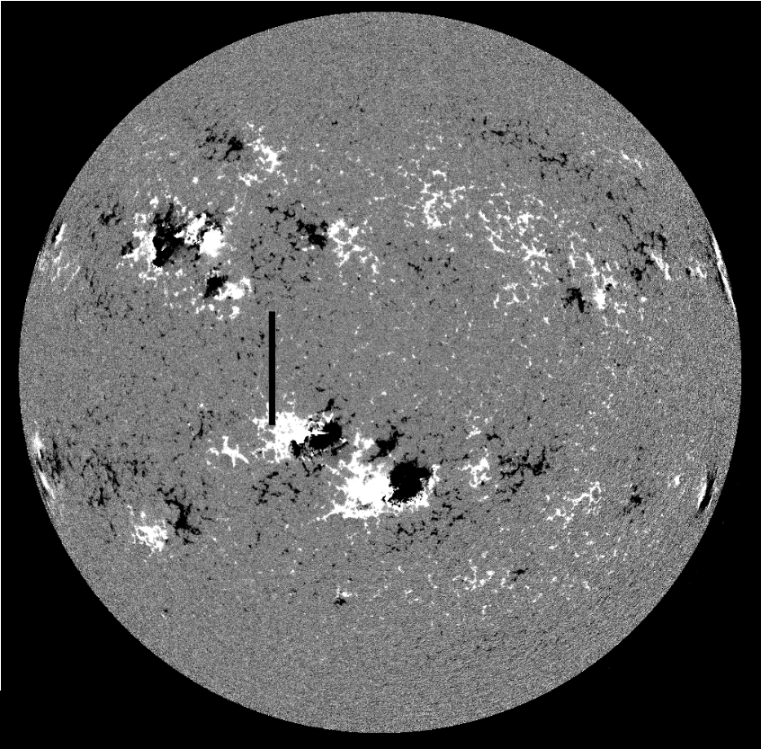
Figure 1: MDI magnetogram of the Sun taken on May 18th at 11:12 UT. The vertical black line marks the approximate position of the SUMER slit in the first time series of spectral images.

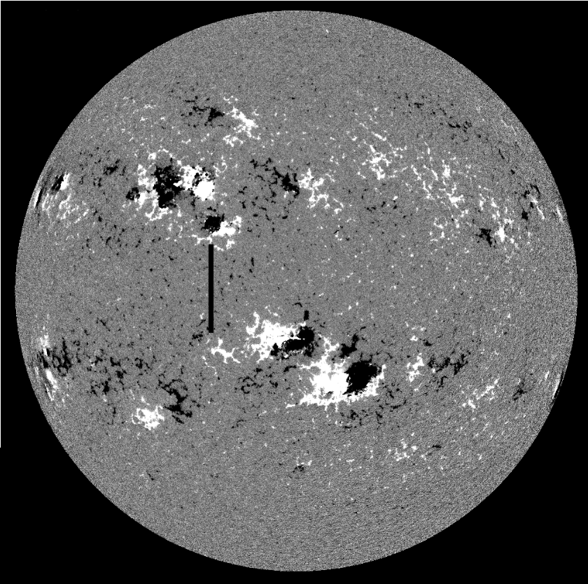
Figure 2: MDI magnetogram of the Sun taken on May 19th at 04:48 UT. The vertical black line marks the approximate position of the SUMER slit in the first time series of spectral images.

3 Methodology

The detection of explosive events recorded in a spectral image has been tackled in the past using differents methods. A precise description of these methos can be found in Pérez et al. (1999), Ning et al. (2004), Teriaca et al. (2004), and Doyle et al. (2006). All these procedures are applied only to a small number of rasters (of the order of a few hundreds), and in most cases the techniques require visual inspection to decide whether a line profile is an explosive event or not. Furthermore, they often consist in hard thresholding the widths or integrated emission of a given spectral line (i.e., they define an explosive event as a line profile with a line width $n\sigma$ above the mean, with $n$ usually 3, and/or equivalently for the line integrated emission). This work presents another perspective based on the idea to allow the data speak for themselves: we implement automatic robust techiques to find outliers in a point distribution where every line profile is characterized by a set of properties parametrizing its non-gaussianity.

Throughout this section we will use the following notation: matrices are denoted by capital letters, often with two subindices that indicate the dimensions of the matrix. For instance, $X_{n,p}$ stands for a matrix with $n$ rows and $p$ columns, where $n$ indexes line profiles and $p$ is the number of variables used to characterise the line profile. These variables are further specified in Sect. 4, but the methodology described below is independent of the choice of variables. A vector is represented by boldface lowercase letter, and it is always assumed to be a column vector. A vector $\mathbf{u}$ with $p$ components is written as $\mathbf{u}=(u_{1},\dots,u_{p})^{T}$.

3.1 The PCOut algorithm

Let $\mathbf{X}$ be a $n\times p$ matrix with each row containing one observation defined by $p$ variables. In our case, each row represents a line profile with $p$ flux values. The PCOut algorithm of Filzmoser et al. (2008) combines two complementary measures of outlyingness (location and scatter outlyingness) to provide a final score that allows the ranking of the observations (the line profiles in our case) according to their deviation from typicality. Observe that typicality refers to quiet sun profiles, and outilers to quiet sun profiles affected by explosive events. That is, letting $F_{1},$ the distribution of the non-outliers and $F_{2}$ the distribution of the outliers, the distribution of the dataset as a whole is usually considered to be given by $F=(1-\epsilon)F_{1}+\epsilon F_{2}$, for $0\leq\epsilon<0.5$. In our problem, $F_{1}$ and $F_{2}$ do not differ so much (disturbances in the profile), and we refer to location outlier if the mean of distribution $F_{2}$ is different from $F_{1}$, and scatter outlier if the variance of $F_{2}$ is different from $F_{1}$.

In the initial step, the algorithm normalises the data using the L1-median as an estimate of the mean and the median absolute deviation (MAD) as an estimate of the standard deviation. The L1-median is a highly robust and orthogonally equivariant location estimator, and it is defined as the point $\theta$ which minimizes the sum of distances to all observations, i.e.

$$\boldsymbol{\mu}=\text{L1MED }(\mathbf{x}_{1},\dots,\mathbf{x}_{n})=\underset{\boldsymbol{\theta}}{\text{argmin }}\,\sum_{i=1}^{n}\|\mathbf{x}_{i}-\mathbf{\boldsymbol{\theta}}\|,$$

where $\|\cdot\|$ stands for the euclidean norm. The MAD is defined for a sample $\{x_{1},\dots,x_{n}\}\subset\varmathbb{R}$ as

$$\text{MAD }(x_{1},\dots,x_{n})=1.4826\cdot\underset{j}{\text{median }}|x_{j}-\underset{i}{\text{median }}x_{i}|$$

Since the MAD is used here as an estimator of the standard deviation $\sigma$, we need to introduce the constant scale factor 1.4826 for consistency. The scale factor ensures that

$$E[MAD(X_{1},\dots,X_{n})]=\sigma,$$

for a random variable $X$ distributed normally as $N(\mu,\sigma^{2})$ and large $n$.

We then compute the sample covariance matrix of the normalised data, $\boldsymbol{C}$, and obtain the principal components of the dataset by selecting the first $q\quad(q<p)$ eigenvectors that contribute at least a preselected percentage (in our case the 99%) of the total variance. From the $q\times q$ matrix $\mathbf{Q}$ of eigenvectors of the sample covariance matrix, we obtain the principal components as

$$\mathbf{Z=X\cdot Q}$$

These principal components are rescaled by the median and the MAD according to,

$$z^{*}_{ij}=\frac{z_{ij}-\text{med}(z_{1j},\dots,z_{nj})}{\text{MAD }(z_{1j},\dots,z_{nj})}$$

3.1.1 Detecting location outliers

The location of the outliers begins by calculating the absolute value of a robust kurtosis measure for each component:

$$w^{*}_{j}=\left|\frac{1}{n}\left(\sum_{i=1}^{n}\frac{(z^{*}_{ij}-\text{med}(z^{*}_{1j},\dots,z^{*}_{nj}))^{4}}{\text{MAD }(z^{*}_{1j},\dots,z^{*}_{nj})^{4}}\right)-3\right|,$$ (1)

where $z^{*}_{ij}$ is $j$-th coefficient of the $i$-th line profile in the new basis of principal components, and $j=1,\dots,q$. In practice we use relative weights $w^{*}_{j}/\sum_{i}w^{*}_{i}$ to produce a standard scale $0\leq w^{*}_{j}\leq 1$.

Equation (1) assigns higher weights to the components where outliers clearly stand out. If no outliers are present in a given component $j$ then we expect the kurtosis to be close to 0, and $w^{*}_{j}\approx 0$. Note that principal components are sorted in decreasing order of explained variance, but also that outliers increase the variance along their respective directions. Therefore: (i) outliers projected over principal components space will be more visible than in the original space, and (ii) we expect outliers to stand out clearly in one principal component rather than being slightly apparent in all of them.

The robust Mahalanobis distances are computed taking into account the weights $w^{*}_{j}$ according to

$$RD_{i}=\sqrt{\sum_{j}(z^{*}_{ij}\cdot w^{*}_{j})^{2}},$$ (2)

The first phase of the algorithm continues with the transformation of the $RD_{i}$ distances according to

$$d_{i}=RD_{i}\cdot\frac{\sqrt{\chi^{2}_{q,0.5}}}{\text{median}\{RD_{i}\}},$$ (3)

where $\chi^{2}_{q,0.5}$ is the $0.5$ quantile of $\chi^{2}_{q}$. The transformation of the robust distances is needed because any resemblance of the $d_{i}$ distribution with a $\chi^{2}_{q}$ distribution is lost with the kurtosis weighting scheme. The distances $d_{i}$ are used to assign weights to each observation by means of the biweight function:

$$w_{1i}=\begin{cases}0,&d_{i}\geq c\\ \left(1-\left(\frac{d_{i}-M}{c-M}\right)^{2}\right)^{2},&M<d_{i}<c\\ 1&d_{i}\leq M\end{cases}$$ (4)

where $i=1,\dots,n$, $M$ is the $0.97$ quantile of the distances $\{d_{1},\dots,d_{n}\}$ and $c$ verifies:

$$c=\text{median}\{d_{1},\dots,d_{n}\}+10\cdot\text{MAD }(d_{1},\dots d_{n}).$$

These weights are used as a measure of location outlyingness.

Note that the values of $M$ and $c$ are not the ones recommended in Filzmoser et al. (2008), but the values that we found to better represent the distribution of SUMER line profiles described above.

3.1.2 Detecting scatter outliers

The second phase of the algorithm is aimed at detecting the so-called scatter outliers, i.e., outliers that do not stand out clearly in one principal component, but that are slightly visible in many of them. Using the same semi-robust principal components decomposition obtained in the first stage of the algorithm, the euclidean norm for data in principal component space is calculated. These distances are equivalent to the Mahalanobis distance in the original data space, and have not been transformed using the kurtosis weighting scheme defined in Eq. (1). Hence, the transformation in Eq. (3) yields a distribution much closer to $\chi^{2}_{q}$. The biweight functions in Eq. (4) are set-up according to the results in Filzmoser et al. (2008), i.e. $M^{2}=\chi^{2}_{q,0.25}$ and $c^{2}=\chi^{2}_{q,0.99}$, except that we need to used quantiles other than 0.25 and 0.99. The values of these quantiles have to be much closer to one in order to better represent a data distribution like ours, where the number of outliers is much smaller that the group of cases defining normality. The weights (measuring scatter outlyingness) calculated in this step are called $w_{2i},\quad i=1,\dots,n$.

3.1.3 Computation of final weights

Finally, the results of the two phases of the algorithm are combined, and final weights $w_{i},\,i=1,\dots,n$ are calculated in accordance with:

$$w_{i}=\frac{(w_{1i}+s)(w_{2i}+s)}{(1+s)^{2}},$$

where typically the scaling constant $s=0.25$. Outliers are then clasified as points having weights $w_{i}<0.25$.

3.2 Wavelet enhanced ICA quiet Sun removal

Once the explosive events are identified by the PCOut algorithm, we want to isolate the explosive event contribution to the line profile from the surrounding quiet Sun emission.

In principle, it can be expected that a line profile revealing an explosive event includes contributions from both the explosion site and the surroundings, in a proportion which is related to the respective volume emission measures and the filling factor. In this section we describe a technique aimed at separating the two contributions.

The Independent Component Analysis (ICA) is a statistical technique for separating a multivariate signal into additive subcomponents, assuming the mutual statistical independence of the non-Gaussian source signals. It can be seen as a special case of the blind source separation problem.

In contrast to Principal Components Analysis, ICA is based on the three following assumptions: (i) the sources are statistically independent; (ii) the probability densities of the sources are non-Gaussian (at most one of them is allowed to be Gaussian); (iii) the mixing of the sources into the observations is linear; and (iv), the number of observations is larger than or equal to the number of sources.

All of these assumptions hold for our data set: (i) it consists of a spatially stable mixture of the activities of temporarily independent quiet Sun and artifactual sources; (ii) the probability densities of the sources are non-Gaussian; (iii) the superposition of the different sources arising from quiet Sun, explosive events, and noise, is linear; and (iv), the number of sources is not larger than the number of wavelengths sampled. The hypothesis of non-Gaussianity of the probability densities is based on the current understanding of the filamentary structure of the Transition Region network, and the bursty nature of explosive events.

Specifically, let there be $p$ signals, $X(t)=\{x_{1}(t),\dots x_{p}(t)\}$, generated as a sum of the $N$ statistical independent components (sources) $S(t)=\{s_{k}(t),\,k=1,\dots,N\}$:

$$\boldsymbol{X}(t)=\boldsymbol{A}\cdot\boldsymbol{S}(t)$$ (5)

where $\boldsymbol{A}$ is the unknown mixing matrix defining the weight of each source. In particular, let $\boldsymbol{X}(t)$ represent the time evolution of the line profile emitted at a particular location in the SUMER slit. Thus, the $\mathbf{x}_{i}(t)$ is the time evolution of the line profile at wavelength $\lambda_{i}$ at that particular location.

For the determination of $\boldsymbol{S}(t)$, we use the FastICA algorithm (Hyvärinen 1999) with the $\log\cosh(\cdot)$  approximation to the negentropy contrast function.

In Sarro & Berihuete (2008) a first version of this method was used. There, we first removed the long timescales component of the time evolution by thresholding the appropriate coefficients in a wavelet decomposition of the original signal. These long time scales were interpreted as the movement of network elements across the slit which occurs in timescales much longer than those typical of explosive events. Then, the signal was decomposed into its independent components and these components sought for explosive events. This proved to be a promising technique for the preprocessing of SUMER data cubes with two main drawbacks: (i) the limitation in the maximal number of independent sources that could be identified, and (ii) the impossibility to find a common ordering of the independent sources found for different slices (positions along the slit) of the data cube, due to intrinsic ambiguities in the ICA algorithms.

To overcome these limitations, we apply here a reversed version of the processing scheme presented in Castellanos & Makarov (2006): first we apply ICA to the data, and then decompose each independent source with a wavelet analysis. Fig. 3 shows the method in a schematic way.

Figure 3: Flow chart of the Wavelet enhanced ICA processing for quiet Sun removal

When we use ICA to identify independent sources, we often find that the explosive events appear in independent components that still contain a significant contribution from typical quiet Sun regions. Let us model these components as the sum of a high amplitude short lived component representative of the activity $s_{1}(t)$, and a long lived low amplitude residual quiet signal $s_{2}(t)$:

$$s_{i}(t)=s_{1i}(t)+s_{2i}(t),$$ (6)

where $s_{i}$ is the original independent component obtained by the ICA algorithm. The objective then, is to estimate the quiet Sun component and subtract it, in order to isolate the explosive event contribution to the line profile.

Note that $s_{1}$ has high magnitude and is very localized in time, while $s_{2}$ has low amplitude and broad band spectrum. We will use the wavelet decomposition technique to separate these signals, providing an optimal resolution both in the time and frequency domains, without requiring the signal to be stationary.

The discrete wavelet transform (DWT) of the independent component $s(t)$ reads:

$$DWT_{s}(j,k;\psi)=\int s(t)\psi_{j,k}(y)\,dt,$$ (7)

where $DWT_{s}(j,k;\psi)$ is the wavelet representation of $s(t)$, $\psi$ is the mother wavelet with $j$ and $k$ defining the time localization and scale,i.e. $\psi_{j,k}(t)=2^{-j/2}\psi(2^{-j}t-k)$. Using Eqs. (6) and (7) we can write:

$$DWT_{s}(j,k;\psi)=DWT_{s_{1}}(j,k;\psi)+DWT_{s_{2}}(j,k;\psi),$$ (8)

where $DWT_{s_{1}}(j,k;\psi)$ and $DWT_{s_{2}}(j,k;\psi)$ are the wavelet coefficients obtained by the transformation of the active and quiet contributions of the independent component respectively.

In order to subtract the quiet Sun component from the original signal, we perform a hard-thresholding of the wavelet coefficients.

The resulting set of thresholded wavelet transform coefficients is inverted, resulting in a denoised version of the original data, with the quiet Sun component removed. Specifically, we use a hard thresholding:

$$\widetilde{DWT}_{s}(j,k;\psi)=\left\{\begin{array}[]{ll}0&|DWT_{s}(j,k;\psi)|\leq T_{j}\\ \vskip 6.0pt plus 2.0pt minus 2.0pt\cr DWT_{s}(j,k;\psi)&\mbox{ otherwise }\end{array}\right.$$ (9)

The threshold is selected based on the universal model of the noise: $T_{j}=\sqrt{2*\log(n)}\,\sigma$. As $\sigma$ is typically unknown, it is estimated based on the median absolute deviation of the absolute value of the wavelet coefficients, i.e. $\sigma^{2}=\mbox{ MAD}(|DWT_{s}(j,k;\psi)|)/0.6745$.

We get separation of the wavelet coefficients into active and quiet Sun, i.e. $DWT_{s_{1}}(j,k;\psi)=0$ then $DWT_{s_{2}}(j,k;\psi)\neq 0$ and viceversa. Then, the wICA-corrected temporal evolution is:

$$\hat{\boldsymbol{X}}(t)=\boldsymbol{A}\cdot(s_{11}(t),s_{12}(t),\dots,s_{1N}(t))^{T}.$$ (10)

Summarising, the wavelet enhanced ICA (wICA) algorithm can be described by the following stages:

1. Apply the conventional ICA decomposition to the time evolution of all monochromatic fluxes, thus obtaining the mixing matrix $\boldsymbol{A}$ and $N$ independent components $\{s_{1}(t),s_{2}(t),\dots,s_{N}(t)\}$.

2. Calculate $DWT_{s_{i}}(j,k;\psi)$ for $i\in\{1,2,\dots,N\}$

3. Threshold the wavelet coefficients.

4. Apply the inverse wavelet transform to the thresholded coefficients $\widetilde{DWT}_{s_{i}}(j,k;\psi)$ to recover only the active component $\{s_{1i}(t)\}$.

5. Signal reconstruction: $\hat{X}(t)=\boldsymbol{A}\cdot(s_{11}(t),s_{12}(t),\dots,s_{1N}(t))^{T}$.

Figure 4 shows the result of applying the wICA algorithm to a slice of the first data cube of observations in the C iv line along the spectral dispersion and time axes. In the top panel we show the original time evolution of the line profiles for a fixed latitude; the middle plot shows the result of applying the wICA filter to the original image, and finally, the bottom panel shows the residual image.

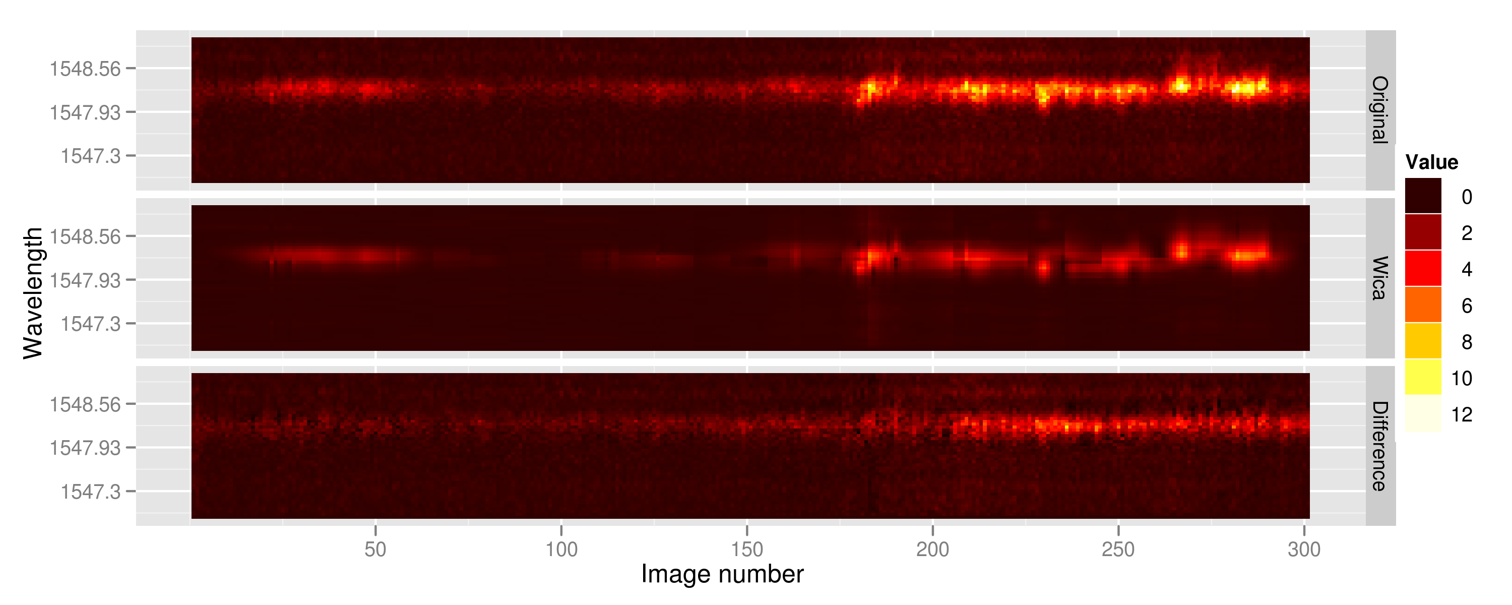
Figure 4: Example of the application of the wICA algorithm to a slice of the data cube showing the time evolution of the C iv line for a fixed position along the slit. From top to bottom we show the original image, the result of the wICA algorithm, and the residual image. The images show time in minutes along the $x$ axis, and wavelength in Angstroms along the $y$ axis.

4 Results

We have applied the techniques described in the previous section to the dataset obtained with SUMER on May 18th and 19th, 2000. The preliminary analysis of the results thus obtained comprised the computation of line radiances, first four line profile moments, and the line profiles maxima. For the outlier detection stage, only the four line profile moments were used in order to rank the rasters according to their non-gaussianity. We intendedly left aside the line radiances and absolute maximum intesities because we did not want to bias the statistical analysis of the explosive events towards the subsample of brightest events.

The $k$-th order moment ($k\geq 2$) of a given raster is defined as

$$m_{k}=\sum_{i}I_{norm,i}(v_{i}-m_{1})^{k}$$ (11)

where $I_{norm,i}$ is the normalised intensity (normalised dividing by the integrated emission in the line profile), $v_{i}$ represents the Doppler velocity, and

$$m_{1}=\sum_{i}I_{norm,i}v_{i}$$ (12)

is the first order moment or weighted mean of the line profile; the summation over $i$ is defined only for values above a 33% of the peak intensity in order to prevent the noise from contaminating the estimate.

One of the advantages of the outlier detection method described in the previous section is that it allows the ranking of line profiles according to the final weights they are assigned. Drawing a line where line profiles are no longer explosive events is difficult, and it may depend on the physcal scenario used to interpret them. We have defined the samples that we will further analyse as those line profiles with final weights below 0.9. This is somewhat arbitrary and we do not claim that all of the line profiles in each sample should unambiguously be considered as an explosive event. In all cases they are composed of line profiles with final weights close to zero which are clearly explosive events under all perspectives, but also of line profiles that outlie the global distribution for reasons that could be explained by correlated noise excursions. We have minimized this sort of ambiguity by imposing thresholds on the signal–to–noise ratio beyond the typical $3\sigma$ limit for the statistical significance of the detection.

As mentioned in Sect. 2, we find evidence that the slit position in both observational sequences covers the external regions of two active regions (NOAA 8998 and NOAA 9004). We have therefore carried out separate studies for the quiet Sun rasters (latitudes below -2^∘ in the first sequence and between $\pm 5^{\circ}$ in the second) and for those potentially affected by the active region (the complementary regions to those defined as quiet Sun).

In the case study of the C iv line we have further restricted the slit positions included in the active region definition. We have detected a systematic shift in the time-averaged line profiles in the data cube slices corresponding to latitudes below -5^∘. The shift increases with decreasing latitude and is due to the appearance of zeros at the short wavelength side of the images. These may affect up to eight consecutive pixels at the lower end of the slit. We interpret this as a problem with the IDL subroutine that corrects for the geometric distorion of the original SUMER image available in the archive. This problem does not affect the Ne viii line where the existence of isolated zeroes at either extreme of the wavelength range does not seem to be correlated with wavelength shifts in the time-averaged line profiles.

In order to define a wavelength scale from the pixel position along the wavelength dispersion axis, we have adopted as reference pixel the one where the maximum emission is attained in the average line profile over all available latitudes and times in the quiet Sun as defined above. We subsequently assigned to this reference pixel, the nominal wavelength of the corresponding line (1548.21 Å  for the C iv line and 770.43; see Dammasch et al. (1999) for a justification of this value). We are perfectly aware that these values are the rest wavelengths for these lines, and that these lines are systematically red shifted in the solar Transition Region. We have prefered to use the rest wavelengths because, as we shall see later, there are significant differences in the distribution of first moments in the scatter plots of the quiet Sun and active regions, and since the aim of this study was not the accurate determination of the transition region systematic redshifts, but the statistical characterization of the explosive event population at small inclinations (i.e. latitudes), we prefered to use a consistent reference wavelength for all regions and lines, and discuss the relative differences amongst them.

The use of the average line profile over all quiet Sun rasters to define the reference pixel for wavelength calibration (instead of the values recorded in the FITS headers) is due to the obvious inconsistency between the reference pixel and the line profiles, that would result in an average line profile red shifted by around 50 km s^-1 if the FITS header values were used.

In Sects. 4.1–4.4 we present the properties of the explosive events in relation with the population of typical quiet Sun line profiles, while in Sect. 4.5 we analyse potential correlations between explosive events properties.

4.1 The C iv line at 1548.2 Å  in the quiet Sun.

We first apply the outlier detection technique described in Sect. 3 to a dataset comprising the regions in the two observational series far from the active regions. As an outcome of this stage we recover a final weight between 0 and 1 assigned to each raster. We group rasters in two categories: typical profiles and outliers. We subsequently use the first category to define the wavelength scale such that the mean quiet Sun line profile is centred at the nominal wavelength of 1548.21 Å.

We show in Figs. 5 and 6 the position of the explosive events in a latitude–time diagram. Since the SUMER slit position was not corrected for solar rotation, this diagram is almost equivalent to a latitude–longitude map except for the non-simultaneity of the measurements. Also, later times in these figures correspond to western latitudes, so the $x$ axis is reversed with respect to Figs. 1 and 2. We have shown in the leftmost panel the line radiance measured between 1547.7 and 1548.7 Åin a logarithmic scale. Then, from left to right, the position of the clear outliers and the first four moments of the line profiles. The kurtosis (fourth moment) is thus the rightmost panel in the figure.

Figure 5: Time-latitude diagram for the first series of observations. In the leftmost panel the total line radiance is shown in a logarithmic colour scale from yellow (lowest) to red (highest values). The next plot to the right shows the same diagram with the position of the quiet Sun C iv outliers superimposed. Finally, form left to right, the same time-latitude diagram with the colour code representing the first, second, third, and fourth order moments in a linear scale.

Figure 6: As Fig. 5 but for the second series of observations.

Neglecting the variations in the solar rotation with latitude, we can covert the total time span of the observations (roughly 5 hours) into an approximate width of 0.17 arcsec/min $\times$ 300 min $\approx$ 50 arcsec. This means that the real observed area is approximately $300^{\prime\prime}\times 50^{\prime\prime}$. The width of each of the images in Figs. 5 and 6 corresponds roughly to this aspect ratio.

Figure 7 shows a scatter plot of the first moment of the line profiles and the integrated line radiances for the significant detections, defined as line profiles with an integrated intensity which exceeds the noise level by $7\sigma$, with $\sigma$ the standard deviation of the continuum level between 1546.9 and 1547.2 Å. This seemingly restrictive threshold is necessary in order to avoid line profiles that are strongly non-gaussian due to noise excursions. The common $3\sigma$ threshold is related to the significance of the detection in the case of a Gaussian signal, but not otherwise. This region is affected by the presence of several Si i lines and therefore the actual signal-to-noise ratio is greater than estimated. We have overplotted the outliers using a colour code that indicates the value of the line profile second order moment, from yellow (lowest values of the second order moment) to red (high values). The scatter plot shows that the vast majority of explosive events concentrate in the low range of line radiances. There are only a few explosive events with radiances above 2 W m^-2 sr^-1, and they are all characterized by large second order moments and net blue shifts. There are hints of a trend in the sense of broader line profiles (redder dots) in the negative side of the $m_{1}$ axis (predominantly blue shifted profiles), although first order moments have to be interpreted with care: if a line profile has three symmetric components (blue, red shifted, and central components) the first moment of the line profile can be vanishingly small even if the separate components arise at significant velocities.

There is one further aspect to be remarked: the asymmetry in the distribution of $m_{1}$ values for line profiles not in the outlier category. It is due to a separate population of low brightness rasters shifted to the red typically by 10–15 km s^-1 with respect to the median value of $m_{1}$ in the sample. The corresponding rasters do not outstand in the distributions of line variance or kurtosis, but are more frequently characterized by negative asymmetries in the third order moments. They thus represent line profiles shifted by up to 30 km s^-1 to the red, with typical line widths, slightly asymmetric, and they appear as outliers if we lower the threshold for outlier detection. If the Doppler shifts were due to the Si i 1548.72 Å satellite line, the line profile would be skewed towards longer wavelengths. This will be interpreted in terms of MHD models of explosive events in Sect. 5.

Figure 7: Distribution of first order moments and radiances in the quiet Sun zones and the two series of observations. The $x$ axis represents the first order moment of the line profile in units of km s^-1, and the $y$ axis, the C iv line radiance in units of W m^-2 sr^-1. Outliers (explosive events) are represented using a colour code indicative of the second order moments of the line profiles.

The total number of outliers is 372, all of them inside the range of integrated intensities defined by the non-outliers, mostly in the low brightness end of the distribution. Therefore, we confirm previous results in the sense that explosive events are not brighter than the typical quiet Sun emission.

Finally, we would like to note that the median wavelength shift is correlated with the integrated intensity averaged over bins, as shown in Fig. 8. The figure shows the median of the first moments obtained grouping the data in bins of integrated intensity. One hundred bootstrap samples are generated in each bin, and the standard deviation of the medians calculated for all the bootstrap samples in each bin, shown as error bars. Except in the first few bins (characterised by small integrated intensities and very populated) the median first order moment is blue shifted, although it has to be recalled that the wavelength calibration is done assuming an average line profile centred at the rest wavelength, and therefore, the actual values have to be taken with caution. It is only the relative differences and the actual correlations that are to be interpreted in the next section. In any case, this proves that the red shifted, blue skewed profiles discussed in previous paragraphs are only a small fraction of the total number of line profiles in the low radiance bins.

Figure 8: The median wavelength shift as a function of the mid-point of radiance bins. The $y$ axis represents the median wavelength shift in units of km s^-1 for several integrated line radiance bins.

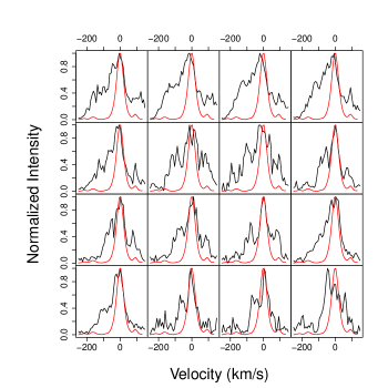
Figure 18: Line profiles in the outlier category of the C iv line in the quiet Sun regions. The average quiet Sun profile is plot in red.

We have included in Fig. 18 plots of the first sixteen elements in the outlier category, with the average quiet Sun profile superimposed in red.

4.2 The C iv line at 1548.2 Å  in the active regions.

Figure 9 shows the radiance–first moment diagram for the latitudes potentially affected by the two active regions NOAA 8998 and NOAA 9004. Using the same definition and thresholds for the outlier detection stage, we find many more extreme events (Doppler velocities of the order of 200 km s^-1). Many of these extreme events appear at small values of the first order moment due to the line symmetry.

Compared to Fig. 7, we find that, in the vicinity of the active regions, the integrated line intensity of both the explosive events and the population of non outliers can be higher by a factor 2.5 with respect to the maximum quiet Sun values. It is important to remark that while the brightest explosive events far from the active regions were significantly dimmer than the maximum radiances encountered in the non outlier category (by a factor 0.5), in the proximities of the active regions the distribution of radiances of explosive events reaches values as bright as those attained in the non-outlier sample.

It is also remarkable the increase in relative importance of the red shifted component amongst the non outliers. While in the quiet Sun we encounter a main distribution centred around the vanishing first order moment line as expected, and an additional component of red shifted line profiles, here the probability density of first order moments in the low radiance regime peaks around 10 km $s^{-1}$ (it has to be recalled that, since the definition of the rasters as belonging to the quiet Sun or active regions is independent of the observational setup, we have used the same reference pixel and dispersion relation in the wavelength calibration of the two sets). Although this effect may be related to the already known difference between the transition region average redshift in the quiet Sun and active regions (see e.g. Teriaca et al. 1999), the magnitude of the difference is larger in our dataset than previously reported.

Figure 9: Distribution of first order moments and radiances in the proximity of the two active regions NOAA 8998 and NOAA 9004. The $x$ axis represents the first order moment of the line profile in units of km s^-1, and the $y$ axis, the C iv integrated line radiance in units of W m^-2 sr^-1. Outliers (explosive events) are represented using a colour code indicative of the second order moments of the line profiles.

Figure 10 shows a similar behaviour in the integrated line radiance as that described in the previous section for the quiet Sun, except for the fact that in the outskirts of the active regions, the correlation/anticorrelation always appears at net red shifts. The behaviour in the last bins is due to the small sample sizes.

Figure 10: The median wavelength shift in the proximity of the two active regions NOAA 8998 and NOAA 9004, as a function of the mid-point of radiance bins. The $y$ axis represents the median wavelength shift in units of km s^-1 for several integrated line radiance bins.

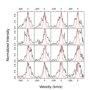
Figure 19: Line profiles in the outlier category of the C iv line in the proximity of the active regions. The average quiet Sun profile is plot in red.

We have included in Fig. 19 plots of the first sixteen elements in the outlier category for the latitudes affected by the active regions.

4.3 The Ne viii line (770.4 Å) line in the quiet Sun.

The Ne viii line at 770.4 Å appears in second order at a wavelength of 1540.85 Å. Figure 11 shows three populations in the integrated line radiance and first order momentum diagram: the bulk of the scatter plot is composed of line profiles centered around the assumed laboratory wavelength as expected (first population); there is also a clear branch of rasters that show a Doppler shift of 20 km s^-1 and radiances greater than or equal to the maximum radiances in the bulk cluster (second population; see Fig. 12 for an example of the brightest profiles in this category); finally, there seems to be evidence for a much smaller cluster of rasters characterized by low radiances and blueshifts between 20 and 40 km s^-1 (third population, shown in colour in Fig. 11).

The second population is characterised by asymmetric line profiles with enhanced blue wings while the third population is composed of 70 rasters with blue shifts equivalent to Doppler velocities greater than 20 km s^-1. Visual inspection of the line profiles in this third category shows that they do not correspond to explosive events. There is no correlation with latitude but they are concentrated in time in the first 30 minutes of the first dataset. The line profiles are asymmetric, with enhanced red wings (as opposed to the second population line profiles). Since their appearance is concentrated in groups of two to four consecutive latitudes and intermittent in time, and they do not show atypical line profile widths, asymmetries or shapes, we interpret them as instrumental shifts occuring at the initial phase of the observations. The outliers of the distribution according to the PCOut algorithm are limited to a number of 47, and they all fall in this third category of blue shifted line profiles .

Figure 11: Distribution of first order moments and radiances of the Ne viii line in the quiet Sun zones. The $x$ axis represents the first order moment of the line profile in units of km s^-1, and the $y$ axis, the Ne viii integrated line radiance in units of W m^-2 sr^-1. Outliers (explosive events) are represented using a colour code indicative of the second order moments of the line profiles.

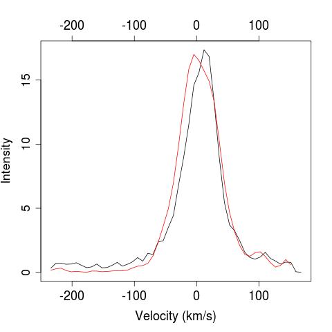
Figure 12: One of the brightest Ne viii line profiles at the tip of the brach of red shifted line profiles in Fig. 11 corresponding to the quiet Sun regions (black). The red line corresponds to the mean line profile in these quiet Sun rasters. The $y$ axis shows the intensity in the Ne viii line in units of W m^-2 sr^-1 Å^-1.

4.4 The Ne viii line at 770.4 Å  in the active regions.

Figure 13 shows the radiance–first moment diagram for the Ne viii line at 770.4 Å in the vicinity of the two active regions NOAA 8998 and NOAA 9004. The diagram is different from the equivalent plot in the quiet regions around the equator, in that the main bulk of rasters is no longer centred around the $m_{1}=0$ vertical line, but around $m_{1}\approx 7$km s^-1, as judged from the histogram.

While the quiet Sun outlier analysis of the Ne viii line at 770.4 Å  did not yield a significant sample of explosive events but only a few tens of blue shifted lines, the rasters in the vicinity of the active regions show significant activity in the form of explosive events. If we examine the sample of outliers, we clearly recognise an imbalance between red and blue asymmetries. The most conspicuous explosive events in the C iv line in quiet Sun and active regions are characterised by predominant blue shifts in their first moments. Explosive events in the Ne viii line, on the contrary, show predominantly red shifted values of $m_{1}$ as shown in Fig. 13. The total number of outliers is 144 (significantly less than the total number of outliers in the C iv outlier category) and although many of them are undoubtedly explosive events, some can be interpreted as line profiles non-gaussian due to noise fluctuations.

Figure 13: Distribution of first order moments and radiances of the Ne viii line in the proximity of the two active regions NOAA 8998 and NOAA 9004. The $x$ axis represents the first order moment of the line profile in units of km s^-1, and the $y$ axis, the Ne viii integrated line radiance in units of W m^-2 sr^-1. Outliers (explosive events) are represented using a colour code indicative of the second order moments of the line profiles.

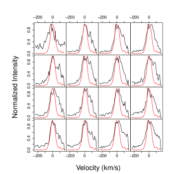
Figure 20: Line profiles in the outlier category of the Ne viii line in the proximity of the active regions. The average quiet Sun profile is plot in red.

We have included in Fig. 20 plots of the first sixteen elements in the Ne viii line outlier category for the latitudes affected by the active regions.

4.5 Properties of the red and blue wings of explosive events

In the following, we analyse and list the properties of the red and blue wings of explosive events line profiles in these new larger samples obtained with the methodology described in Sect. 3. We hope that this summary of the statistical properties of the new samples will help guide future numerical simulations of explosive events, by pointing to the observational trends, or absence of correlations that need be reproduced or explained by them.

We have defined the red (blue) wing as the line profile to the right (left) of the rest wavelength (as defined above) in the wICA denoised spectral images. The red edge of the spectral images correspond to a Doppler red shift of approximately 150 km s^-1, while the blue edge blue shift is sensibly larger ($\approx$ -250 km s^-1) due to the rest wavelength not being centred in the window. In the following, we study the red and blue spectral line wings in two windows 150 km s^-1 wide at each side of the rest wavelength. For each window we compute the line radiance ($F_{red}$, $F_{blue}$), the first and second line moments ($m_{1,red}$, $m_{1,blue}$, m_2,red, and $m_{2,blue}$), and the velocity at which the 20% of the maximum line intensity is first attained. These latter values (one for each wing) are taken as indicative of the maximum Doppler shifts. We believe that the characterisation of explosive events involves all of these parameters. Apparently, the second order moments carry similar information to the velocities at the 20% of the maximum flux, but careful visual examination of the explosive events shows that this is not the case, and we can find very different line profiles with roughly equal second order moments. In some cases the line profile can be decomposed into several resolved components, but never is a gaussian fit an adequate description for them.

First, we concentrate in the distribution of radiances in the samples. Figures 14 and 15 show the distribution of radiances in the red and blue windows and in the three study cases with significant amounts of explosive events, i.e., the quiet Sun regions in the C iv line, and the regions in the proximities of active regions NOAA 8998 and NOAA 9004 in C iv and Ne viii. The scatter plots and histograms show hints that the quiet Sun explosive events in the C iv line are composed of two populations: one with brighter red wings which is more numerous in the fainter end of the distribution of total radiances) and one with blue wings brighter which dominates the population at the bright end of the distribution. In the proximities of the active regions, explosive events with brighter red wings still dominate the faint end of the distribution, but the situation in the bright end is balanced. Finally, the situation in the Ne vii line is different, with predominantly red explosive events dominating both at the faint and bright ends, and predominantly blue events being more frequent at intermediate radiances.

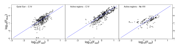
Figure 14: Scatter plots of the radiance emitted in the red and blue wings ($x$ and $y$ axes respectively) of explosive events in the quiet Sun Civ line profiles (left panel), and near the active regions in C iv (middle) and Ne viii (right).

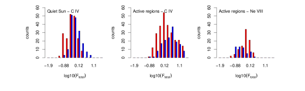
Figure 15: Histograms of the number of explosive events in bins of the total line radiance. Red bars correspond to explosive events with red wings brighter than the blue wings, and blue bars, to blue wings brighter than the red ones. The left and central panels correpond to the C iv line in the quiet and active regions respectively, and the rightmost panel shows the same histogram for the Ne viii line in the vicinity of the active regions.

Next, we concentrate in the distribution of maximum velocities and their correlation with the total line radiance. Figure 16 represents the Doppler shift at which the line profile decays down to the 20% of the maximum in the red and blue wings (the colour code reflects the total line radiance in a logarithmic scale). This is used as an indicator of the maximum velocities that characterise the explosive event. In the quiet Sun regions (leftmost plot), the scatter plot shows a tendency for the C iv lines to have larger maximum blue shifts than maximum red shifts (explosive events above the diagonal) except in the region of small velocities (below 75 km s^-1) where maximum red shifts larger than the maximum blue shifts are more frequent (a situation similar to that found in Fig. 15 for the wing brightness). Brighter events tend to show larger maximum velocities as expected, and the brightest events in this category have maximum velocities which are larger in the blue window.

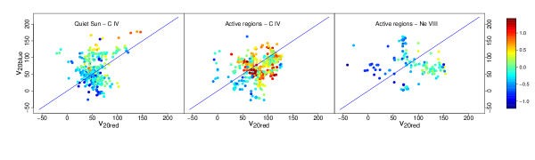
Figure 16: Scatter plots of the velocities at which the 20% of the maximum line profile is attained at each side of the maximum emission ($x$- and $y$- axes respectively). The left and central plots correspond to the C iv line in the quiet Sun regions and in the proximities of the active regions; the rightmost scatter plot corresponds to the Ne viii line in the proximities of the active regions. The colour code represents the total flux radiance in a logarithmic scale. Blue correponds to the lowest values of the line radiance while red corresponds to the highest values.

In the scatter plot corresponding to the C iv line in the proximities of the active regions, larger maximum red shifts are systematically more numerous, and there seems to be a separation at $v_{20}\approx$60–70 km s^-1. Explosive events with maximum velocities larger than these values are brighter and less asymmetric on average. It is interesting to note that the two scatter plots showing explosive events in the C iv line are complementary, with quiet Sun explosive events densely populating the lower left corner of the diagram and active region explosive events occupying preferentially the adjacent region to the upper right.

In the Ne viii line profiles in the outskirts of the active regions, explosive events show a butterfly diagram with explosive events characterized by maximum red shifts larger than the maximum blue shifts being both brighter and slightly more numerous than the opposite. Line profiles that are totally contained in one of the two windows only occur in the faint end of the radiance distribution, and appear in these plots with negative values in one of the axes.

Finally in Fig. 17 we analyse the distribution of first order moments in relation with the line variance (second order moment). The $x$ and $y$ axes show the values of the first order moment of the red and blue wings of the line profile (as defined above), and the colour code represents the value of the difference between the second order moments $d_{2}=m_{2,red}-m_{2,blue}$. Figure 17 shows a remarkable difference with respect to Fig. 16. While the Ne viii and quiet Sun C iv distributions show basically the same structure in the two figures, the distribution of C iv explosive events in the proximities of the active regions shows that profiles that appear with small first order moments (lower left corner in the middle panel of Fig. 17) are characterised by large maximum velocities $v_{20}$, and thus, appear at the upper right corner in the middle panel of Fig. 16.

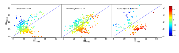
Figure 17: First moments ($m_{1}$) of the red and blue windows at each side of the rest wavelength ($x$ and $y$ axes respectively). The colour code represents the second order moment of the red wing minus the second order moment of the blue one. Blue correponds to the lowest values of the difference while red corresponds to the highest values. The plots show, from left to right, the C iv line in the quiet Sun and the C iv and Ne viii lines in the vicinity of the active regions.

In particular, it is worth noting the presence of several explosive events characterized by large positive values of $d_{2}$, $m_{1,red}$, and $m_{1,blue}$ in the C iv–active regions panel of Fig. 17, breaking the general trend that $d_{2}$ isarithms run parallel to the $m_{1,red}=m_{1,blue}$ line. They correspond to explosive events with one distinct emission component in the blue wing (and thus a narrow main velocity component), and extended emission in the red wing that we interpret as arising from plasma with a wide distribution of velocities which actually extends beyond the maximum velocity in the blue window. We have included in Fig. 21 a few examples of this category with the aim of helping in the interpretation of the $m_{1}$–$m_{2}$ diagrams.

5 Discussion

The first result that we would like to discuss is the fact that the red wings are neither sistematically brighter than the blue ones, nor slower. This is nevertheless a common prediction from the simulations which is explained in Heggland et al. (2009): red wings arise from plasma streams travelling in a medium denser than the medium encountered by the plasma responsible for the blue wing emission, and thus, since they propagate at the Afvén speed, they are characterized by smaller velocities. This is expected in stratified media, with density decreasing towards the observer. Furthermore and for the same reason, the plasma receding from the observer is compressed leading to enhanced emission.

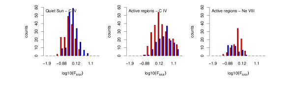
Figure 22: Histograms of the number of explosive events in bins of total line radiance. Similar to Fig. 15, but here for velocity thresholds: red bars correspond to explosive events with maximum velocities in the red wing larger than the corresponding blue maximum velocity, and blue bars to larger maximum velocities in the blue.

The problem arises in the interpretation of the low radiance explosive events in the quiet Sun rasters: their red wings are brighter than the blue ones as expected, but their maximum Doppler shifts in the red wing are also larger than the maximum blue shifts, as shown in Figs. 16 and 22. The opposite also applies: the brightest events have larger maximum Doppler shifts in the blue wing as expected, but also more flux in the blue wings, and this is also not predicted by the simulations.

Our interpretation of the results shown in the previous sections is a complex scenario where explosive event properties are defined by several elements. The most important one is the magnetic flux available for reconnection. This is evident from the comparison of the characteristics of the explosive events in the quiet Sun and near the active regions in Fig. 16, that the properties of the line profiles are almost complementary, to the extent that the small overlap of explosive events near the active regions showing characteristics of low energy events and viceversa can be explained as due to the coarseness of the definition of quiet Sun and active region. The fact that the available magnetic flux is an important ingredient in explosive events is not new: the fact that its influence dominates over that of others is.

The analysis of the next important element that defines the properties of explosive events is, unfortunately, beyond the present observational capabilities: it is the small scale geometry of the magnetic field that dictates the directions of the plasma jets. As shown by Heggland et al. (2009), the picture of two aligned jets can only be applied to the reconnection site, and different moving angles can occur after the jets have interacted with the surrounding medium. Furthermore, the reconnection geometry varies with time depending on the phase of the driving mechanism.

If different deflection angles for the two reconnection jets were indeed the reason for the unexpected larger maximum velocities in the red wing, it would imply that the emission detected as explosive events comes mainly, not from the reconnection site, but from regions where interaction with the surrounding medium has already changed the direction of the flow. More simulations with different initial magnetic field configurations are needed in order to explore this hypothesis.

The height above the solar photosphere where magnetic reconnection occurs is also another important ingredient. The effect of a height variation is twofold. Down in the chromosphere, the expected Alfven velocity is smaller, and emission from both the reconnection site and the plasma flows receding from it will appear combined in the same spectrograph element for a longer time. But also, densities in the chromosphere are higher than at the base of the Transition Region and therefore higher radiances should be expected. We have not found evidence for this correlation between larger line radiances and smaller maximum velocities, and therefore we must conclude that either the explosive events cannot be triggered in a wide range of heights, or the correlation is masked by other effects.

In general, we find that the brightest C iv explosive events are also characterised on average by larger maximum velocities. If the enhanced line radiances were due to a chromospheric origin, we would expect small maximum velocities, and since this is not the case, we interpret them as due to a larger amount of magnetic energy ready to be tranformed into kinetic energy and heating. But we find marginal evidence in the middle panel of Fig. 16 that the brightest events, even if the occupy the region of large maximum velocities, tend to cluster around $v_{max}\approx$70 km s^-1. This could be an indication that the two mechanisms are taking place: near the active regions there is more magnetic energy available and thus, explosive events are brighter, but at the same time they occur preferentially at lower heights in the chromosphere and, as a consequence, they are bright but relatively slow compared to events with the same available energy but triggered higher in the atmosphere.

Finally, we are tempted to interpret the population of gaussian red shifted profiles in the quiet Sun in C iv (see Fig. 7) as a population of low energy explosive events occuring deep in the chromosphere. But the lack of blue wing enhancements at all possible line radiances argues against this hypothesis.

6 Conclusions

In this work we have presented a totally automated processing of homogeneous series of spectral images taken by the SUMER spectrograph on board SOHO. As a result, we have several samples of explosive events in the two lines of C iv and Ne viii, in regions of the quiet Sun and in the outer parts of two active regions. The main objective of this work was to advance in the analysis of explosive events by looking at the general properties of the samples rather than studying individual cases.

The main conclusions from our work are that

• even though we have significantly enlarged the sample size of explosive events by automating its detection, no clear and unique picture emerges, capable of describing the variety of line profiles encountered and described in Sect. 4.5;

• current numerical simulations fail to explain the existance of explosive events line profiles with blue components much brighter than their red counterparts, and/or with maximum Doppler velocities in the red wing much larger than in the blue one;

• the characteristics of explosive events near active regions as compared to their quiet Sun counterparts, and in particular their maximum velocities, cannot be explained only as the result of enhanced magnetic flux available for reconnection.

This work leaves many unanswered questions. In particular, we have not analysed the time evolution of the explosive events, nor have we correlated the position of explosive events near the two active regions in the C iv and Ne viii lines. We intend to explore these issues in the future, together with the latitude dependence of the sample properties or the impact of the time resolution by comparing this dataset with others available in the SOHO data archive.

Figure 21: Atypical examples of C iv explosive events in the proximities of the active regions NOAA 8998 and NOAA 9004. The $y$ axis shows the line intensity in units of W m^-2 sr^-1 Å^-1.