Magnetic field generated by r-modes in accreting quark stars

Abstract

We show that the r-mode instability can generate strong toroidal fields in the core of accreting millisecond quark stars by inducing differential rotation. We follow the spin frequency evolution on a long time scale taking into account the magnetic damping rate in the evolution equations of r-modes. The maximum spin frequency of the star is only marginally smaller than in the absence of the magnetic field. The late-time evolution of the stars which enter the r-mode instability region is instead rather different if the generated magnetic fields are taken into account: they leave the millisecond pulsar region and they become radio pulsars.

I Introduction

Since the first paper in which r-modes in rotating neutron stars were shown to be unstable with respect to the emission of gravitational waves Andersson:1997xt , it was recognized their relevance in Astrophysics to explain the observed distribution of the rotation frequency of stars in Low-Mass-X-Ray-Binaries (LMXBs) (see Andersson:2000mf for a review). On the other hand, the instability triggered by r-modes is actually damped to some extent by the viscosity of the matter composing the star: the higher the viscosity, the higher is the frequency of rotation of the star. This fact opens the possibility of investigating the internal composition of compact stars by studying the viscosity of the different possible high density phases which can appear in these stellar objects. A number of papers are currently present in the literature about the shear and bulk viscosities of nucleonic matter Sawyer:1989dp ; Haensel:1992zz ; Haensel:2000vz ; Haensel:2001mw ; Benhar:2007yj , hyperonic matterLindblom:2001hd ; Haensel:2001em ; Chatterjee:2006hy ; Chatterjee:2007iw ; Gusakov:2008hv ; Sinha:2008wb ; Jha:2010an , kaon condensed matter Chatterjee:2007qs ; Chatterjee:2007ka , pure quark phases Madsen:1992sx ; Madsen:1999ci ; Alford:2006gy ; Sa'd:2006qv ; Sa'd:2007ud ; Alford:2007rw ; Blaschke:2007bv ; Sa'd:2008gf ; Mannarelli:2008je ; Jaikumar:2008kh ; Alford:2009jm , and mixed phases Drago:2003wg . Interestingly, by studying the so called “window of instability” of the r-modes, which is determined by the shear and the bulk viscosity of the matter, it was pointed out in Drago:2007iy that a detection of a sub-millisecond rotating star would indicate the existence of a very viscous phase in the star with only quark or hybrid stars as possible candidates.

Also the temporal evolution of the spin frequency of a star under the effect of r-modes instability has been studied for different types of composition and different physical systems: newly born compact stars and old stars in binaries Lindblom:1998wf ; Owen:1998xg ; Andersson:2001ev ; Wagoner:2002vr ; Drago:2004nx ; Drago:2007iy . While neutron stars could be very powerful gravitational waves emitter only during their first months after birth Owen:1998xg , hyperonic and quark or hybrid stars could turn into steady gravitational waves sources if present in LMXBs Andersson:2001ev ; Wagoner:2002vr ; Reisenegger:2003cq .

R-modes are also responsible for differential rotation in the star which in turn generates a toroidal magnetic field: besides the viscosity of matter, the production of this magnetic field represents a very efficient damping mechanism for the r-modes. This effect has been proposed and investigated in Rezzolla2000ApJ ; Rezzolla:2001di ; Rezzolla:2001dh for the case of a newly born neutron star and it has been recently included within the r-mode equations of the neutron stars in LMXB Cuofano:2009xy ; Cuofano:2009yg : by calculating the back-reaction of the magnetic field on the r-modes instability, it has been proven that magnetic fields of the order of $10^{15}$ G can be produced. Remarkably, this mechanism could be at the origin of the enormous magnetic field of magnetars.

In this paper we extend the calculations of Cuofano:2009xy ; Cuofano:2009yg to the case of quark stars in LMXB. The motivation for this investigation is that the evolution of accreting stars and their internal magnetic field depends strongly on the r-modes instability window which, for quark stars, is qualitatively different from the one of neutron star. Indeed, due to the large contribution to the bulk viscosity of the non leptonic weak decays occurring in strange quark matter, the window of instability splits into two windows, a small one at large temperatures (which is actually irrelevant for the evolution) and a big one at low temperatures Madsen:1999ci ; Drago:2007iy . Moreover, quark stars do not have a crust (or just a very thin crust) and, as we will discuss, this prevents the trapping of the internal magnetic field developed during the evolution with possible observable signatures.

The paper is organized as follows: in Sec. II we introduce the system of equations which provide the temporal evolution of a compact star in a LMXB. In Sec. III we show the results of our numerical calculations and finally in Sec. IV we present of conclusions.

II The temporal evolution model

II.1 R-modes equations

Let us review the derivation of the equations for the evolution of a compact star in presence of the r-modes.
Following the discussion of Ref. Wagoner:2002vr , we start from the conservation of the angular momentum. The total angular momentum of the star can be decomposed into an equilibrium angular momentum $J_{*}$ and a canonical angular momentum $J_{c}$, proportional to the r-modes amplitude $\alpha$:

$$J_{tot}=J_{*}+(1-K_{j})J_{c}$$

$$J_{c}=-K_{c}\alpha^{2}J_{*}$$ (1)

where $J_{*}=I_{*}\Omega$, with $\Omega$ the angular velocity and $I_{*}=\tilde{I}MR^{2}$ the moment of inertia of a star of mass $M$ and radius $R$. For a n=1 polytrope $\tilde{I}=0.261$, $K_{c}=9.4\times 10^{-2}$ (see Ref. Owen:1998xg ) and $K_{j}$ is of the order of unity (the results of our calculations are rather insensitive to the value of $K_{j}$).

The equations for the evolution of a star are based on two simple considerations:

• the canonical angular momentum, proportional to the r-modes amplitude, increases with the emission of gravitational waves and decreases due the presence of damping mechanisms (as e.g. viscosity and the torque due to an internal magnetic field $B$):

  $$\frac{dJ_{c}}{dt} = 2J_{c}\big{(}\frac{1}{\tau_{GW}(M,\Omega)}$$ (2)

  $$- \frac{1}{\tau_{damp}(M,\Omega,T,B)}\big{)}$$

  where $\tau_{GW}(M,\Omega)$ and $\tau_{damp}(M,\Omega,T,B)$ are the gravitational wave emission timescale and the damping timescale, respectively, where the latter includes all the mechanisms muffling the r-modes. Finally with $T$ we mean the average temperature of the star.

• the total angular momentum takes contributions from the mass accretion and decreases due to the emission of gravitational waves and electromagnetic waves. The electromagnetic wave emission is associated to the presence of an external poloidal magnetic field which is not aligned with the rotation axis. Indicating with $\tau_{m_{e}}$ the braking timescale due to the external magnetic field, the second equation reads:

  $$\frac{dJ_{tot}}{dt}=\frac{2J_{c}}{\tau_{GW}}+\dot{J}_{a}-\frac{J_{*}}{\tau_{m_{e}}}$$ (3)

  where $\dot{J}_{a}$ is the variation of the angular momentum due to the mass accretion. Following Ref. Andersson:2001ev , we assume $\dot{J}_{a}=\dot{M}(GMR)^{1/2}$.

Combining together the equations (1), (2) and (3), it is easy to obtain the evolution equations for $\Omega$ and for the r-modes amplitude $\alpha$:

$$\frac{d\alpha}{dt} = \alpha\big{(}\frac{1}{\tau_{GW}}-\frac{1}{\tau_{damp}}\big{)}$$ (4)

$$+ K_{c}\alpha^{3}\big{[}K_{j}\frac{1}{\tau_{GW}}+(1-K_{j})\frac{1}{\tau_{damp}}\big{]}$$

$$- \frac{\alpha\dot{M}}{2\tilde{I}\Omega}\big{(}\frac{G}{MR^{3}}\big{)}^{1/2}+\frac{\alpha}{2\tau_{m_{e}}}$$

$$\frac{d\Omega}{dt} = -2K_{c}\Omega\alpha^{3}\big{[}K_{j}\frac{1}{\tau_{GW}}+(1-K_{j})\frac{1}{\tau_{damp}}\big{]}$$ (5)

$$- \frac{\dot{M}\Omega}{M}+\frac{\dot{M}}{\tilde{I}}\big{(}\frac{G}{MR^{3}}\big{)}^{1/2}-\frac{\Omega}{\tau_{m_{e}}}$$

Here we adopt the estimate given in Ref. Andersson:2000mf for the gravitational radiation rate due to the $l=m=2$ current multipole:

$$\frac{1}{\tau_{GW}}=\frac{1}{47}M_{1.4}R_{10}^{4}P_{-3}^{-6}\quad s^{-1}$$ (6)

where we have used the notation $M_{1.4}=M/1.4M_{\odot}$, $R_{10}=R/10$ km and $P_{-3}=P/1$ ms.

Following Ref. Cuofano:2009yg , the total damping rate is given by the sum of the shear viscosity and bulk viscosity rates plus the damping rate due to the internal magnetic field:

$$\tau_{damp}^{-1}=\tau_{s}^{-1}+\tau_{b}^{-1}+\tau_{m_{i}}^{-1}$$ (7)

The estimates of the viscosity damping rates for the case of pure quark matter are given in Ref. Andersson:2001ev . For the shear viscosity it is found:

$$\tau_{s}=3.4\times 10^{9}\alpha_{s}^{5/3}M_{1.4}^{-5/9}R_{10}^{11/3}T_{9}^{5/3}\quad s$$ (8)

where $\alpha_{s}$ is the strong coupling constant and $T_{9}=T/10^{9}$ K. For the bulk viscosity, the viscosity coefficient takes the form

$$\zeta=\frac{\tilde{\alpha}T^{2}}{\omega^{2}+\beta T^{4}}$$ (9)

where $\omega$ is the frequency of the r-modes in the corotating frame and $\tilde{\alpha}$ and $\beta$ are coefficients given in Ref.Madsen:1992sx . Due to this behavior, bulk viscosity is very large at $T\sim 10^{9}K$ and gets weaker at both lower and higher temperatures. The instability window is then splitted into a Low Temperature Window (LTW) (at $T<10^{9}$ K) and an High Temperature Window (HTW) ($T>10^{9}$ K). Due to the fast cooling rate of quark stars, the (HTW) is crossed very rapidly and does not have a big impact on the evolution of the star. So we are interested only in the LTW. The bulk viscosity damping timescale in the low temperature limit ($T<10^{9}$ K) is given byAndersson:2001ev :

$$\tau_{b}^{low}=7.9M_{1.4}^{2}R_{10}^{-4}P_{-3}^{2}T_{9}^{-2}m_{100}^{-4}\quad s$$ (10)

where $m_{100}$ is the mass of the strange quark in units of 100 MeV. Notice that the value bulk viscosity damping timescale is strongly dependent on the value of $m_{100}$.

The expression of the magnetic damping rate has been derived in Rezzolla:2001di ; Rezzolla:2001dh , where it has been shown that while the star remains in the instability region, the r-modes generate a differential rotation which can greatly amplify a pre-existing magnetic field. More specifically, if a poloidal magnetic field was originally present, a strong toroidal field is generated inside the star. The energy of the modes is therefore transferred to the magnetic field and the instability is damped.
We assume that the internal stellar magnetic field B is initially based on the solution obtained by Ferraro Ferraro1954ApJ which can be written Cuofano:2009yg

$$\mbox{{B}}_{0}^{in}(t=0)=$$ (11)

$$B_{d}\,\left[\left(-3\frac{r^{2}}{R^{2}}+5\right)\texttt{cos}\,\theta\,\mbox{{e}}_{r}+\left(6\frac{r^{2}}{R^{2}}-5\right)\,\texttt{sin}\,\theta\,\mbox{{e}}_{\theta}\right]\,.$$

where $B_{d}$ is the strength of the equatorial magnetic field at the stellar surface.
To estimate the magnetic field produced by r-modes we start by writing the $l=m=2$ contribution to the perturbation velocity:

$$\delta\textbf{v}(r,\theta,\phi,t)=\alpha\Omega R\left(\frac{r}{R}\right)^{2}\textbf{Y}_{22}^{B}e^{i\sigma t}.$$ (12)

Following Ref. Rezzolla:2001di we get the total azimuthal displacement from the onset of the oscillation at $t_{0}$ up to time $t$, which reads:

$$\Delta\tilde{x}^{\phi}(r,t)\equiv\int_{t_{0}}^{t}\delta v^{\phi}(t^{\prime})dt^{\prime}$$

$$=\frac{2}{3}\left(\frac{r}{R}\right)k_{2}(\theta)\int_{t_{0}}^{t}\alpha^{2}(t^{\prime})\Omega(t^{\prime})dt^{\prime}+\mathcal{O}(\alpha^{3})\,\,\,\,\,\,\,\,\,$$ (13)

where $k_{2}(\theta)\equiv(1/2)^{7}(5!/\pi)(\texttt{sin}^{2}\theta-2\texttt{cos}^{2}\theta)$. The relation between the new and the original magnetic field inside the star in the Lagrangian approach reads Rezzolla:2001di :

$$\frac{B^{j}}{\rho}(\tilde{\textbf{x}},t)=\frac{B^{k}}{\rho}(\textbf{x},t_{0})\frac{\partial\tilde{x_{j}}(t)}{\partial x^{k}(t_{0})}.$$ (14)

This equation implies that the radial dependence of the initial and final magnetic field is the same. Integrating on time the induction equation in the Eulerian approach one gets Rezzolla:2001dh :

$$\delta B^{\theta} \simeq \delta B^{r}\simeq 0$$

$$\delta B^{\phi} \simeq B_{0}^{\theta}\int\dot{\phi}(t^{\prime})dt^{\prime}\simeq B_{0}^{\theta}\int\frac{\delta v^{\phi}(t^{\prime})}{r}dt^{\prime}$$ (15)

where $B_{\phi}$ is the toroidal component.
The expression of the magnetic damping rate reads Cuofano:2009yg :

$$\frac{1}{\tau_{m_{i}}(t)} = \frac{(dE_{M}/dt)}{\tilde{E}}$$ (16)

$$\simeq \frac{4\int_{0}^{2\pi}d\phi\int_{0}^{\pi}k_{2}^{2}(\theta)\texttt{sin}\theta d\theta\int_{0}^{R}r^{4}B^{2}(r,\theta)dr}{9\pi\cdot(8.2\times 10^{-3})MR^{4}\Omega}$$

$$\times \int^{t}_{0}\alpha^{2}(t^{\prime})\Omega(t^{\prime})dt^{\prime}\,\,\,\,\,\,\,\,\,\,\,$$

$$\simeq \frac{4A}{9\pi\cdot(8.2\times 10^{-3})}\frac{B_{d}^{2}R\int^{t}_{0}\alpha^{2}(t^{\prime})\Omega(t^{\prime})dt^{\prime}}{M\Omega}\,\,\,\,\,\,\,\,\,\,\,$$

where $\tilde{E}$ is the energy of the mode, $E_{M}$ is the magnetic energy and $A\approx 0.99$. The time integral over the r-mode amplitude $\alpha$ takes contribution from the period during which the star is inside the instability region.

II.2 Temperature evolution

The equations derived above are strongly dependent on the value of the temperature, therefore we need to compute also the thermal evolution of the star. For the sake of simplicity we assume that the temperature is uniform in the star and we make use of the estimates derived in Ref. Andersson:2001ev , for the case of quark stars. The heat capacity reads:

$$C_{V}=1.5\times 10^{38}M_{1.4}^{2/3}R_{10}T_{8}\quad erg/K$$ (17)

The star cools down essentially by emitting neutrinos, through the so called URCA processes. Taking into account the direct URCA process, which are likely to occur in the core of quark stars, the cooling rate due to emission of neutrinos reads: Andersson:2001ev :

$$\dot{E}_{neutrino}=3.77\times 10^{37}R_{10}^{3}T_{8}^{6}\quad erg/s$$ (18)

If the star is accreting mass then one has to consider the heating due to the accreted material. In particular, for a quark star the heating source comes from the conversion of nucleons into strange matter. Estimating the energy release from this conversion to be around 20 MeV per nucleon Alcock:1986hz ; Andersson:2001ev , the heating rate due to the accretion is given by:

$$\dot{E}_{accretion}=1.19\times 10^{37}\dot{M}_{-8}\quad erg/s$$ (19)

where $\dot{M}_{-8}$ is the accretion rate in units of $10^{-8}M_{\odot}$ per year. The last contribution to the heating of the star comes from the viscosity. Taking into account the contributions of both bulk and shear viscosity, the associated heating rate reads Owen:1998xg :

$$\dot{E}_{viscosity}=2\alpha^{2}\Omega^{2}MR^{2}\tilde{J}\big{(}\frac{1}{\tau_{s}}+\frac{1}{\tau_{b}}\big{)}\quad erg/s$$ (20)

where the expression for $\tau_{s}$ and $\tau_{b}$ are given in eqs. (8) and (10), respectively, and $\tilde{J}=(2/3)\times 9.4\times 10^{-2}\tilde{I}$.

Finally, the equation for the thermal evolution of the star is given by:

$$\frac{d}{dt}\big{(}\frac{1}{2}C_{V}T\big{)}=\dot{E}_{accretion}+\dot{E}_{viscosity}-\dot{E}_{neutrino}$$ (21)

In the absence of r-modes, the temperature is determined by a balance between accretion heating and neutrino cooling:

$$T=8.25\times 10^{7}\big{(}\dot{M}_{-8}R_{10}^{-3}\big{)}^{1/6}K$$ (22)

III Results and discussion

By solving the Eqs.(4,5,16,21) it is possible to obtain the temporal evolution of quark stars, taking into account the formation of toroidal magnetic fields due to r-mode instability. In particular, in the present work we show the results only for the case of quark stars inside of LMXBs. Eq. (15) gives the strength of the new toroidal component created by the winding up of a pre-existent poloidal field, due to the differential rotation induced by r-modes. Several issues remain open concerning the way the new magnetic fields, produced by the damping of the r-modes, are affected by possible instabilities. In the stably stratified matter of a stellar interior there are two types of instabilities: the Parker (or magnetic buoyancy) and the Tayler instabilities (or pinch-type), both driven by the magnetic field energy in the toroidal field. The condition for the Tayler instability to set in is given by 1999A&A…349..189S ; 2002A&A…381..923S :

$$\frac{\omega_{A}}{\Omega}>\big{(}\frac{N_{\mu}}{\Omega}\big{)}^{1/2}\big{(}\frac{\eta}{r^{2}\Omega}\big{)}^{1/4}$$ (23)

where $\omega_{A}=B/(4\pi\rho)^{1/2}r$ is the Alfven frequency, $N_{\mu}\simeq 5\times 10^{4}s^{-1}$ is the compositional contribution to the buoyancy frequency and $\eta\sim 10^{-9}f(m_{s})T_{8}^{2}cm^{2}s^{-1}$ is the magnetic diffusivity which can be obtained from the electrical conductivity $\sigma$ by using the relation $\eta=1/(\mu_{0}\sigma)$ Haensel:1991pi and $f(m_{s})$ takes into account the dependence of the electron fraction on the mass of the strange quark and it ranges from $11$ to $4$ to $2.5$ when $m_{s}$ changes from $100$ to $200$ to $300$ MeV. From Eq. (23) we can conclude that in a pure quark star, the Tayler instability sets in for $B>B_{cr}\sim 10^{12}$ G. After the development of the Tayler instability, the toroidal component of the field produces, as a result of its decay, a new poloidal component which can then be wound up itself, closing the dynamo loop. When the differential rotation stops the field can evolve into a stable configuration of a mixed poloidal-toroidal twisted-torus shape inside the star with an approximately dipolar field connected to it outside the star 2006A&A…449..451B ; 2004Natur.431..819B ; 2006A&A…450.1097B ; 2006A&A…450.1077B . Concerning the buoyancy instability, it occurs for $B_{cr}\gtrsim 10^{15}$ G Haensel:2007tf , therefore it is not relevant in our calculations.

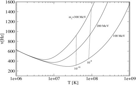
Figure 1: The quark star instability window for three values of the strange quark mass. The dashed lines indicate the evolution of a star in a LMXB during the accretion stage up to the moment in which the star enters the instability window.

It is very important to point out that the formation and the further stabilization of magnetic fields in the core of compact stars, leads to different scenarios depending of the star composition. For instance, neutron stars contain a highly conductive crust acting as a screen for the internal large magnetic field. Conversely, whether quark stars contain or not a crust is still controversial. Various types of crust have been suggested: a tenuous crust made of ions suspended on the electric field associated with the most external layer of a quark star Alcock:1986hz ; a crust made of a mixed phase of electrons and of quark nuggets Jaikumar:2005ne ; a crust made of a mixed phase of hadronic and quark matter Drago:2001nq . The electric properties of the crust area strongly connected with the electron density, which is suppressed in the core (what has been taken into account above, while discussing the magnetic diffusivity) and which can be enhanced in the crust, at least in the model in which a fraction of hadron is present in the crust Drago:2001nq . Although detailed calculations of the structure of the crust of a quark star are not yet available, we can assume that if a crust exists its electric properties interpolate between those of a normal neutron star and those of a bare quark star, the two limiting situations.
As discussed above, when Tayler instability sets in, a poloidal component with strength similar to the toroidal one ($B\sim 10^{12}$ G) is generated. If the crust is not present (the case with a crust will be shortly discussed later in the conclusions) such large poloidal component is not screened and diffuses outside of the star, preventing the star from further accreting mass. Therefore, following this scenario, if a quark star inside of a LMXB produces, due to the r-mode instability, an internal magnetic field larger than the Tayler instability threshold, then it should stop accreting mass. Thus this represents, at least in principle, an additional constraint on the highest rotational frequency of the compact stars in LMXBs.

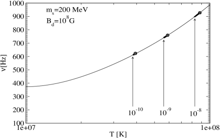
Figure 2: Instability window and trajectories of the evolution of the frequency and temperature of the star for different values of the mass accretion rate. The short thick lines represent the paths followed by the star after the instability windows is touched. The dots indicate the onset of the Tayler instability at which the evolution is stopped.

There are many parameters that enter into the equations for the temporal evolution of the frequency of the star. We fix the mass and the radius of the star to be $1.4M_{\odot}$ and $10$ km respectively. A crucial quantity for the bulk viscosity is the mass of the strange quark for which we will consider the three values $m_{s}=100-200-300$ MeV. The smallest value for $m_{s}$ is basically the current mass of the strange quark as used within MIT bag-like models and the last value is compatible with results of chiral quark models as the NJL model. The astrophysical input parameters concern the mass accretion rate, for which we use the values in the range $(10^{-10}-10^{-8})\,\mbox{M}_{\odot}\mbox{yr}^{-1}$, and the initial dipolar magnetic field varied in the interval ${\bf B_{0}}=10^{8}-10^{9}$ G.

Let us start our discussion with the r-modes instability window shown in Fig. 1. With increasing values of $m_{s}$, the bulk viscosity increases and therefore the instability region becomes smaller. Also shown by dashed lines are the trajectories of the evolution of a star in a LMXB during the accretion stage and until the star enters the instability window for two extreme values of the mass accretion ($10^{-10}$ and $10^{-8}$ $M_{\odot}yr^{-1}$ ).
The evolution is calculated by starting from a configuration below the instability window: an initial value of $100-200$ Hz is taken as initial frequency, $\alpha$ is set to zero and the initial temperature is the equilibrium temperature as expressed by Eq.(22). Due to accretion, the star is spun up until it reaches the instability window and at that point the r-modes instability starts to develop. The bulk viscosity dissipates part of the r-mode energy into heat with a consequent reheating of the star and the internal magnetic field starts to grow. At the same time, the frequency of the star continues to grow due to the accretion torque, and the amplitude of the r-modes increases. The simultaneous effect of reheating and accretion leads the star to follow the border of the instability window. This is clearly shown in Fig. 2, where the thick lines indicate the paths followed by the star (for different values of the accretion rate) and the dots, at which the evolution stops, signal the onset of the Tayler instability. The temporal evolution of the r-modes amplitude is shown in Fig. 3 and Fig. 4, where we take $m_{s}=100$ MeV and $m_{s}=200$ MeV, respectively. For both the cases the initial dipolar magnetic field has a value of $10^{8}$ G.

Figure 3: Temporal evolution of $\alpha$ for different values of the mass accretion rate. Here the initial poloidal magnetic field is $B_{d}=10^{8}$ G and $m_{s}=100$ MeV.

Figure 4: As in Fig. 3 with $m_{s}=200$ MeV.

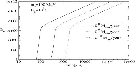
Figure 5: Temporal evolution of the internal toroidal magnetic field $B_{\varphi}$ for different values of the mass accretion rate. Here $B_{d}=10^{8}$ G and $m_{s}=100$ MeV.

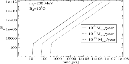
Figure 6: As in Fig. 5 with $m_{s}=200$ MeV.

Notice that after an initial stage in which $\alpha$ oscillates (the star enters and exits the instability region), $\alpha$ then increases steadily but its value is still so small that r-modes cannot reach the saturation regime. So our calculations are independent of the value of $\alpha$ in the saturation regime. Parallel to the evolution of $\alpha$ we show in Figs. 5 and 6 the temporal evolution of the internal magnetic field. As expected, the value of $B_{\phi}$ follows the same evolution of $\alpha$. Again, we stopped the evolution as soon as $B_{\phi}$ reaches the threshold for the Tayler instability $B_{cr}\sim 10^{12}$ G.

As discussed in Ref. Andersson:2001ev , in which the effect of internal magnetic damping was not considered, a quark star inside a LMXB can be spun up up to a maximum frequency, corresponding to the frequency at which the accretion torque balances the spin down torque due to the emission of gravitational waves. However, taking into account the internal magnetic damping, a quark star without a crust should stop accreting after the onset of Tayler instability is reached. Therefore an important question is how much the limiting frequency is reduced with respect to the case in which the internal magnetic field is not taken into account. To this purpose, we computed the maximum frequencies for both the cases, estimating in this way the effect of the internal magnetic field. These frequencies are shown in Fig. 7 as a function of $m_{s}$ and for two values of the initial poloidal magnetic field, $B_{d}=10^{8}$ G (dashed line) and $B_{d}=10^{9}$ G (dot-dashed line). Notice that the effect of the internal magnetic field is rather small, reducing the maximum rotational frequency only by a few tens Hertz. Moreover, the proven existence of stars in LMXBs rotating at frequencies larger than $600$ Hz rules out a value of $m_{s}\sim 100$ MeV.

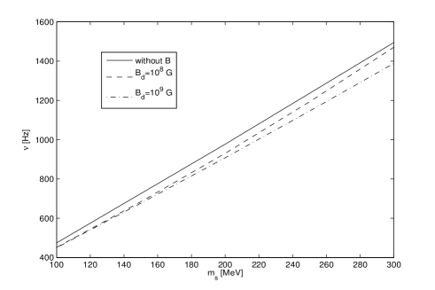
Figure 7: Maximum spin frequencies of quark stars as a function of the mass of the strange quark. The results obtained assuming a initial poloidal magnetic field $B_{d}=10^{8}$ G (dashed line) and $B_{d}=10^{9}$ G (dot-dashed line) are compared to the result obtained without the internal magnetic field (solid line).

Finally, we investigate the possible evolutionary scenarios of quark stars beyond the onset of the Tayler instability. Let us first consider a star without a crust: as soon as the Tayler instability sets in, the new magnetic configuration prevents the star from further accreting mass. The new poloidal component, of the same order of magnitude of the toroidal component ($\sim 10^{12}$ G), will act as a strong braking torque, and the star will lose angular momentum. Such evolutionary path is plotted in the plane $P\mbox{--}\dot{P}$ in Fig.(8) and is depicted by the green line. It is very interesting to notice that, starting from the region of LMXBs, the star evolves into the region of radio pulsars.

On the contrary, a highly conductive crust could screen the internal magnetic field for a very long time. A possible example of such a crust is that described in Ref. Drago:2001nq where the most external layer is made of an admixture of hadrons and quarks. In that case the electron fraction (and therefore also the electric conductivity) is large in the crust and decreases towards to core of the star. The evolution of the star depends on the dominant dissipation mechanism associated with the crust. The most relevant one is probably the ambipolar diffusion (see Refs. Cuofano:2009xy ; Cuofano:2009yg ), whose typical timescale is:

$$t_{ambip}\sim 3\times 10^{9}\frac{T_{8}^{2}L_{5}^{2}}{B_{12}^{2}}yr$$ (24)

, where $L_{5}=L/10^{5}$ cm is the size of the region embedding the magnetic field. Due to this diffusion mechanism, the internal magnetic field can “quite rapidly” (in a few millions years) diffuse outside of the crust, and also in this case the star should stop accreting. In the meanwhile, the external magnetic field should spin down the star. In Fig. 8 we indicate with a blue line a sketch of the path followed by the star when the ambipolar diffusion is present; also in this case the star evolves into the region of the radio pulsars.

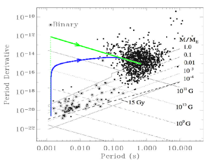
Figure 8: Trajectories in the plane $P\mbox{--}\dot{P}$ of quark stars after the development of the Tayler instability. The green line corresponds to a quark star without a crust; the blue line is obtained if in the crust the main diffusive process is the ambipolar diffusion.

It is important to remark that the time spent by the quark star after the Tayler instability and before it reaches the region of the radio pulsars is of the order of a few million years, to be compared with the time spent inside the radio pulsar region, which is of the order of a few hundreds million years. Therefore we can expect that only a few percent of the stars following the trajectory indicated in Fig(8) will be detected before reaching the radio pulsar region.

IV Conclusions

We have shown that strong toroidal fields can be generated in the core of an accreting millisecond quark star which enters the r-mode instability window. Tayler instability sets in when the generated toroidal fields exceed the critical value $B_{tor}^{cr}\sim 10^{12}$ G and a new poloidal component of similar strength is produced. Our results show that the maximum spin frequency for quark stars does not change significantly when taking into account the internal generated magnetic fields.
The scenario after the development of the Tayler instability depends on the presence and the properties of a possible crust. If the crust is not present, the generated large poloidal component diffuses quickly outside the core and prevents the further accretion of mass on the star. On the other hand, if a highly conductive crust is present, it could screen to some extent the internal magnetic field. However, taking into account the ambipolar diffusion, which is, in this case, the dominant dissipation mechanism, the star could expel the internal magnetic field in a few millions years, which would then stop the accretion. In both cases the quark star evolves into the region of radio pulsars, as shown in Fig.8: this represents a new possible scenario for the formation of radio pulsars.

- (1) N. Andersson, Astrophys. J. 502, 708 (1998), arXiv:gr-qc/9706075
- (2) N. Andersson and K. D. Kokkotas, Int. J. Mod. Phys. D10, 381 (2001), arXiv:gr-qc/0010102
- (3) R. F. Sawyer, Phys. Rev. D39, 3804 (1989)
- (4) P. Haensel and R. Schaeffer, Phys. Rev. D45, 4708 (1992)
- (5) P. Haensel, K. P. Levenfish, and D. G. Yakovlev, Astron. Astrophys. 357, 1157 (2000), arXiv:astro-ph/0004183
- (6) P. Haensel, K. P. Levenfish, and D. G. Yakovlev, Astron. Astrophys. 327, 130 (2001), arXiv:astro-ph/0103290
- (7) O. Benhar and M. Valli, Phys. Rev. Lett. 99, 232501 (2007), arXiv:0707.2681 [nucl-th]
- (8) L. Lindblom and B. J. Owen, Phys. Rev. D65, 063006 (2002), arXiv:astro-ph/0110558
- (9) P. Haensel, K. P. Levenfish, and D. G. Yakovlev, Astron. Astrophys. 381, 1080 (2002), arXiv:astro-ph/0110575
- (10) D. Chatterjee and D. Bandyopadhyay, Phys. Rev. D74, 023003 (2006), arXiv:astro-ph/0602538
- (11) D. Chatterjee and D. Bandyopadhyay, Astrophys. J. 680, 686 (2008), arXiv:0712.3171 [astro-ph]
- (12) M. E. Gusakov and E. M. Kantor, Phys. Rev. D78, 083006 (2008), arXiv:0806.4914 [astro-ph]
- (13) M. Sinha and D. Bandyopadhyay, Phys. Rev. D79, 123001 (2009), arXiv:0809.3337 [astro-ph]
- (14) T. K. Jha, H. Mishra, and V. Sreekanth, Phys. Rev. C82, 025803 (2010), arXiv:1002.4253 [hep-ph]
- (15) D. Chatterjee and D. Bandyopadhyay, Phys. Rev. D75, 123006 (2007), arXiv:astro-ph/0702259
- (16) D. Chatterjee and D. Bandyopadhyay(2007), arXiv:0712.4347 [astro-ph]
- (17) J. Madsen, Phys. Rev. D46, 3290 (1992)
- (18) J. Madsen, Phys. Rev. Lett. 85, 10 (2000), arXiv:astro-ph/9912418
- (19) M. G. Alford and A. Schmitt, J. Phys. G34, 67 (2007), arXiv:nucl-th/0608019
- (20) B. A. Sa’d, I. A. Shovkovy, and D. H. Rischke, Phys. Rev. D75, 065016 (2007), arXiv:astro-ph/0607643
- (21) B. A. Sa’d, I. A. Shovkovy, and D. H. Rischke, Phys. Rev. D75, 125004 (2007), arXiv:astro-ph/0703016
- (22) M. G. Alford, M. Braby, S. Reddy, and T. Schafer, Phys. Rev. C75, 055209 (2007), arXiv:nucl-th/0701067
- (23) D. B. Blaschke and J. Berdermann, AIP Conf. Proc. 964, 290 (2007), arXiv:0710.5243 [hep-ph]
- (24) B. A. Sa’d(2008), arXiv:0806.3359 [astro-ph]
- (25) M. Mannarelli, C. Manuel, and B. A. Sa’d, Phys. Rev. Lett. 101, 241101 (2008), arXiv:0807.3264 [hep-ph]
- (26) P. Jaikumar, G. Rupak, and A. W. Steiner, Phys. Rev. D78, 123007 (2008), arXiv:0806.1005 [nucl-th]
- (27) M. G. Alford, M. Braby, and S. Mahmoodifar, Phys. Rev. C81, 025202 (2010), arXiv:0910.2180 [nucl-th]
- (28) A. Drago, A. Lavagno, and G. Pagliara, Phys. Rev. D71, 103004 (2005), arXiv:astro-ph/0312009
- (29) A. Drago, G. Pagliara, and I. Parenti, Astrophys. J. 678, L117 (2008), arXiv:0704.1510 [astro-ph]
- (30) L. Lindblom, B. J. Owen, and S. M. Morsink, Phys. Rev. Lett. 80, 4843 (1998), arXiv:gr-qc/9803053
- (31) B. J. Owen et al., Phys. Rev. D58, 084020 (1998), arXiv:gr-qc/9804044
- (32) N. Andersson, D. I. Jones, and K. D. Kokkotas, Mon. Not. Roy. Astron. Soc. 337, 1224 (2002), arXiv:astro-ph/0111582
- (33) R. V. Wagoner, Astrophys. J. 578, L63 (2002), arXiv:astro-ph/0207589
- (34) A. Drago, G. Pagliara, and Z. Berezhiani, Astron. Astrophys. 445, 1053 (2006), arXiv:gr-qc/0405145
- (35) A. Reisenegger and A. A. Bonacic, Phys. Rev. Lett. 91, 201103 (2003), arXiv:astro-ph/0303375
- (36) L. Rezzolla, F. K. Lamb, and S. L. Shapiro, Astrophys. J. 531, L139 (Mar. 2000)
- (37) L. Rezzolla, F. K. Lamb, D. Markovic, and S. L. Shapiro, Phys. Rev. D64, 104013 (2001)
- (38) L. Rezzolla, F. K. Lamb, D. Markovic, and S. L. Shapiro, Phys. Rev. D64, 104014 (2001)
- (39) C. Cuofano and A. Drago, J. Phys. Conf. Ser. 168, 012008 (2009), arXiv:0903.0349 [astro-ph.HE]
- (40) C. Cuofano and A. Drago, Phys. Rev. D82, 084027 (2010), arXiv:0905.3368 [astro-ph.HE]
- (41) V. C. A. Ferraro, Astrophys. J. 119, 407 (Mar. 1954)
- (42) C. Alcock, E. Farhi, and A. Olinto, Astrophys. J. 310, 261 (1986)
- (43) H. C. Spruit, Astron. Astrophys. 349, 189 (Sep. 1999), arXiv:astro-ph/9907138
- (44) H. C. Spruit, Astron. Astrophys. 381, 923 (Jan. 2002), arXiv:astro-ph/0108207
- (45) P. Haensel, Nucl. Phys. Proc. Suppl. 24B, 23 (1991)
- (46) J. Braithwaite, Astron. Astrophys. 449, 451 (Apr. 2006), arXiv:astro-ph/0509693
- (47) J. Braithwaite and H. C. Spruit, Nature 431, 819 (Oct. 2004), arXiv:astro-ph/0502043
- (48) J. Braithwaite and H. C. Spruit, Astron. Astrophys. 450, 1097 (May 2006), arXiv:astro-ph/0510287
- (49) J. Braithwaite and Å. Nordlund, Astron. Astrophys. 450, 1077 (May 2006), arXiv:astro-ph/0510316
- (50) P. Haensel and J. L. Zdunik, Nuovo Cim. B121, 1349 (2006), arXiv:astro-ph/0701258
- (51) P. Jaikumar, S. Reddy, and A. W. Steiner, Phys. Rev. Lett. 96, 041101 (2006), arXiv:nucl-th/0507055
- (52) A. Drago and A. Lavagno, Phys. Lett. B511, 229 (2001), arXiv:hep-ph/0103209