Electromagnetically induced Talbot effect

Abstract

By modulating transmission function of a weak probe field via a strong control standing wave, an electromagnetically induced grating can be created in the probe channel. Such a nonmaterial grating may lead to self-imaging of ultra-cold atoms or molecules in the Fresnel near-field regime. This work may offer a nondestructive and lensless way to image ultra-cold atoms or molecules.

Optical imaging offers a powerful diagnostic methodology for a variety of experiments involving ultra-cold atoms and molecules. Two methods, on/off-resonant absorption imaging, are often chosen to image the atomic or molecular cloud. On-resonant absorption imaging ketterle is predominant, despite its limited dynamic range and recoil heating. Although off-resonant phase-imaging techniques dobrek allow nondestructive and quantitative imaging of Bose-Einstein condensates (BECs), traditional approaches usually require precisely aligned phase plates or interferometers. In this paper, we propose another type of lensless imaging scheme, electromagnetically induced Talbot effect (EITE) or electromagnetically induced self-imaging (EISI), for ultra-cold atoms and molecules. This work might broaden variety applications in imaging techniques and be useful for atom lithography atom as well.

The proposed scheme to conduct lensless imaging of ultra-cold atoms and molecules relies on periodically manipulating transmission and dispersion profiles of a weak probe field under the condition of electromagnetically induced transparency (EIT).EIT1 ; EIT2 The basic idea is to utilize a strong control standing wave to modify the optical response of the medium to the weak probe field, i.e., electromagnetically induced grating.EIG Such an induced nonmaterial grating thus leads to self-images of atoms and molecules in the Fresnel diffraction region. Conventional Talbot effect talbot1 ; talbot2 ; case relates the self-imaging of periodic objects without using any optical components. Images observed in the Fresnel near-field regime are repeated along or backward along the illumination direction depending on whether the light is transmitted or reflected. Recent renewed interest in this remarkable phenomenon, Talbot effect, is motivated by the progress made on atomic waves,pritchard BECs,phillips quantum carpets,berry , Gauss sums,schleich x-ray phase imaging,david nonclassical light,wen1 and second harmonic generation.wen2 ; wen22

To be specific, we consider a medium of length $L$ consisting of an ensemble of closed three-level ultra-cold atoms (or molecules) in the $\Lambda$ configuration, with two metastable lower states, as shown in Fig. 1(a). Two ground states $|b\rangle$ and $|c\rangle$ are coupled to the excited state $|a\rangle$ via a strong control field of angular frequency $\omega_{c}$ near resonance on the $|c\rangle\rightarrow|a\rangle$ transition with a detuning $\Delta_{c}=\omega_{c}-\omega_{ac}$, and a weak probe field of angular frequency $\omega_{p}$ close to resonance on the $|b\rangle\rightarrow|a\rangle$ transition with a detuning $\Delta_{p}=\omega_{p}-\omega_{ab}$. The control light consists of two fields which are symmetrically displaced with respect to $z$ and whose intersection generates a standing wave within the medium, see Fig. 1(b) and the snapshot [Fig. 1(c)]. To introduce the notations, we denote the amplitude of the probe field as $E_{p}$ and its Rabi frequency as $\Omega_{p}$. For simplicity, hereafter we assume that two cw control fields share the same Rabi frequency $\Omega_{c}$. $\gamma_{a}$ and $\gamma_{bc}$ are the decay rate of excited state $|a\rangle$ and dephasing rate between two ground states $|b\rangle$ and $|c\rangle$, respectively. Initially, all the population is distributed in the ground state $|b\rangle$.

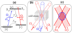
Figure 1: (Color online) (a) A closed three-level $\Lambda$-type atomic system for EITE. (b) Configuration of forming an EIG. (c) Snapshot of the EIG in (b).

The linear susceptibility of the system at the probe frequency is now

$$\chi=\frac{N|\mu|^{2}}{2\hbar\epsilon_{0}}\frac{\Delta_{2}+i\gamma_{bc}}{|\Omega_{c}|^{2}\cos^{2}\big{(}\frac{{\pi}x}{a}\big{)}-(\Delta_{p}+i\gamma_{a})(\Delta_{2}+i\gamma_{bc})},$$ (1)

where $\Delta_{2}=\Delta_{p}-\Delta_{c}$ is the two-photon detuning and $a$ is the spatial period of the standing wave along the $x$ direction perpendicular to the propagation direction $z$. In principle, $a$ can be made arbitrarily larger than the wavelength $\lambda_{p}$ of the probe field by varying the angle between the two wave vectors of two control beams. The propagation dynamics of the probe field within the cloud obeys the Maxwell’s equation and its transmission at the output surface is

$$E_{p}(x,L)=E_{p}(x,0)e^{-\frac{k_{p}\chi^{\prime\prime}}{2}L}e^{i\frac{k_{p}\chi^{\prime}}{2}L},$$ (2)

where $\chi=\chi^{\prime}+i\chi^{\prime\prime}$ and $E_{p}(x,0)$ is the input probe profile. For simplicity, the probe field is assumed to be a plane wave. Figure 2(a) displays two typical profiles of the probe field at the output surface as $\Delta_{p}=\Delta_{2}=0$. At the transverse locations around the nodes (of the standing wave), the probe beam is absorbed according to the usual Beer law because the control field intensity there is very weak. In contrast, at the transverse locations around the antinodes, the probe is absorbed much less due to the EIT effect. This leads to a periodic amplitude modulation across the probe profile, a phenomenon reminiscent of the amplitude grating. If the probe field is detuned off the resonance, a phase modulation will be also introduced to its output profile. Figure 2(b) shows, over several periods, the transmission function $|E_{p}(L,x)|$ (upper curve) and phase $\Phi$ (lower curve) as $\Delta_{p}=2\gamma_{a}$ and $\Delta_{c}=0$. At nodes, the probe field experiences a rapid phase change in contrast to Fig. 2(a) where no phase modulation is introduced.

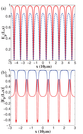
Figure 2: (Color online) The output profile of the probe field, $E_{p}(L,x)$, as a function of $x$. (a) An amplitude grating: optical depth $=20$, $\Omega_{c}=10\gamma_{a}$ (upper curve) and optical depth $=4$, $\Omega_{c}=3\gamma_{a}$ (lower curve). Other parameters are $\Delta_{p}=\Delta_{2}=0$, $\gamma_{bc}=0.3\gamma_{a}$, and $a=10$ $\mu$m. (b) A hybrid grating: optical depth $=8$, $\Delta_{p}=2\gamma_{a}$, $\Delta_{c}=0$, $\Omega_{c}=10\gamma_{a}$, and $\gamma_{bc}=0.3\gamma_{a}$.

Using the Fresnel-Kirchhoff diffraction integral, the output probe field $\mathscr{E}_{p}$ at a distance $Z$ from the output surface of the medium is proportional to

$$\mathscr{E}_{p}(X,Z)\propto\int^{\infty}_{-\infty}E_{p}(x,L)e^{ik_{p}(Z+\frac{x^{2}}{2Z}-\frac{xX}{Z}+\frac{X^{2}}{2Z})}dx,$$ (3)

where $x$ and $X$ are the coordinates in the object and observation planes, respectively. From Eq. (3) the diffraction amplitude $\mathscr{E}_{p}(X,Z)$ is determined by $E_{p}(x,L)$. For conventional Talbot effect, if $E_{p}$ is a one-dimensional periodic function, self-imaging of the object then repeats at every Talbot plane. In fact, because of the periodicity exhibited in Eq. (1) it may be recast into Fourier series,

$$E_{p}(x,L)=\sum^{+\infty}_{n=-\infty}C_{n}e^{i2\pi{n}\frac{x}{a}},$$ (4)

where $C_{n}$ is the coefficient of the $n$th harmonic. Its detailed format may be obtained by setting $y=e^{i2\pi\frac{x}{a}}$, representing $C_{n}$ in terms of the contour integral around the unit circle, and calculating the residue at 0. By substituting Eq. (4) into (3) and completing the integral, we recover the traditional Talbot effect,

$$\mathscr{E}_{p}(X,Z)\propto\sum^{+\infty}_{n=-\infty}C_{n}e^{-i\frac{\pi\lambda_{p}n^{2}Z}{a^{2}}}e^{i\frac{2\pi{n}X}{a}}.$$ (5)

Some conclusions are immediately in order from Eq. (5). First, in the planes $Z_{T}=ma^{2}/\lambda_{p}$, where $m$ denotes a positive integer referred to as the self-imaging number, the field amplitude matches the amplitude at the output plane of the ensemble $z=L$. At these planes, all the diffraction orders are in phase. In the case of $m$ being odd integers, the self-images are shifted half a period with respect to the even-number orders. Second, the localization of the planes with best visibility is independent of the magnitude of the phase modulation due to the EIT effect. It coincides with the self-image planes. In general, the axial repetition period $a^{2}/\lambda_{p}$ of the Fresnel diffraction is preserved. Third, there are no planes where only images of phase modulation occur.

The validity of Eq. (4) can be verified by numerically evaluating Eq. (3) with use of (2). For instance, in Fig. 3(a) we gave the spatial distribution of the diffraction amplitude at the first Talbot plane ($m=1$) by setting $\Delta_{p}=\Delta_{2}=0$, i.e., an amplitude grating. From the figure, it is obvious that the object image is shifted laterally half a period with respect to the output profile of the probe field [see Fig. 2(a)], which agrees with the theoretical prediction described above. This further proves the correctness of Eq. (4) using the Fourier series expansion, which allows the analytical analysis on the effect. The visibility at the Talbot planes approaches almost unity in such an amplitude-grating case. The spatial profile of the diffracted probe beam at the $m=1$ plane shown in Fig. 3(b) gave another case that by detuning it off the resonance, an induced hybrid (both amplitude and phase) grating can be generated and experienced by the input probe light. One can notice that the location of the Talbot plane coincides with the amplitude-grating case and is independent of the introduced phase modulation, except the maximum amplitude contrast is decreased [compared with Fig. 2(b)]. All of these agree well with the prediction drawn from Eq. (5).

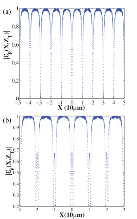
Figure 3: Self-imaging of the output probe field, $|\mathscr{E}_{p}(X,Z_{T})|$, observed at the first Talbot plane ($m=1$). (a) An amplitude grating: parameters are chosen as optical depth $=20$, $\Omega_{c}=10\gamma_{a}$, $\Delta_{p}=\Delta_{2}=0$, $\gamma_{bc}=0.3\gamma_{a}$, and $a=10$ $\mu$m. (b) A hybrid grating: optical depth $=8$, $\Omega_{c}=10\gamma_{a}$, $\Delta_{p}=2\gamma_{a}$, $\Delta_{c}=0$, $\gamma_{bc}=0.3\gamma_{a}$, and $a=10$ $\mu$m.

In summary, we theoretically propose an idea to image the cold atoms with EITE. The effect is capable of lensless imaging and may reduce the influence from vibrations in the experiment. Thus it could be useful for imaging BEC on chip hansel ; du and optical lattice. In practice, the imaging quality may be affected by the finite dimensions of the standing wave and the size of the input probe field. For visible light, the Talbot length here is about several tenth of millimeters. Therefore, a second imaging process would be necessary to magnify the self-images as implemented in Ref.wen2 We also notice that our scheme might be possible to study the nonspreading wave packets as demonstrated in Ref. stutzle . Further development of this proposal will be presented elsewhere. Besides, our recent research kerr indicate that such a configuration is also useful for quantum information science.

We gratefully acknowledge helpful discussions with M. H. Rubin and Yan-Hua Zhai. J.W. and M.X. were supported in part by the National Science Foundation (USA). J.W. also acknowledges financial support from China by 111 Project B07026. S.D. was supported by the Hong Kong Research Grants Council (Project No. HKUST600809).

References

- (1) M. R. Andrews et al, Science 275, 637 (1997).
- (2) L. Dobrek et al, Phys. Rev. A 60, R3381 (1999).
- (3) G. Timp et al, Phys. Rev. Lett. 69, 1636 (1992).
- (4) S. E. Harris, Phys. Today 50 (7), 36 (1997).
- (5) M. Xiao et al, Phys. Rev. Lett. 74, 666 (1995).
- (6) H. F. Talbot, Philos. Mag. 9, 401 (1836).
- (7) K. Patorski, Progress in Optics 27, pp. 1-108, edited by E. Wolf (North-Holland, Amsterdam, 1989).
- (8) W. P. Case et al, Opt. Express 17, 20966 (2009).
- (9) M. S. Chapman et al, Phys. Rev. A 51, R14 (1995).
- (10) C. Ryu et al, Phys. Rev. Lett. 96, 160403 (2006).
- (11) C. David, B. Nohammer, H. H. Solak, and E. Ziegler, Appl. Phys. Lett. 81, 3287 (2002).
- (12) M. V. Berry, I. Marzoli, and W. P. Schleich, Phys. World 14, 39 (2001).
- (13) D. Bigourd et al, Phys. Rev. Lett. 100, 030202 (2008).
- (14) K.-H. Luo et al, Phys. Rev. A 80, 043820 (2009).
- (15) Y. Zhang et al, Phys. Rev. Lett. 104, 183901 (2010).
- (16) J.-M. Wen et al, J. Opt. Soc. Am. B 28, 275 (2011).
- (17) H. Y. Ling, Y.-Q. Li, and M. Xiao, Phys. Rev. A 57, 1338 (1998).
- (18) W. Hänsel, P. Hommelhoff, T. W. Hänsch, and J. Reichel, Nature (London) 413, 498 (2001).
- (19) S. Du et al, Phys. Rev. A 70, 053606 (2004).
- (20) R. Stützle et al, Phys. Rev. Lett. 95, 110405 (2005).
- (21) J.-M. Wen et al, Phys. Rev. A 82, 043814 (2010).