The Role of the IGIMF in the chemical evolution of the solar neighbourhood

Abstract

The integrated galactic initial mass function (IGIMF) is computed from the combination of the stellar initial mass function (IMF) and the embedded cluster mass function, described by a power law with index $\beta$. The result of the combination is a time-varying IMF which depends on the star formation rate. We applied the IGIMF formalism to a chemical evolution model for the solar neighbourhood and compared the results obtained by assuming three possible values for $\beta$ with the ones obtained by means of a standard, well-tested, constant IMF. In general, a lower absolute value of $\beta$ implies a flatter IGIMF, hence a larger number of massive stars, higher Type Ia and II supernova rates, higher mass ejection rates and higher [$\alpha$/Fe] values at a given metallicity. Our suggested fiducial value for $\beta$ is 2, since with this value we can account for most of the local observables. We discuss our results in a broader perspective, with some implications regarding the possible universality of the IMF and the importance of the star formation threshold.

1 Introduction

The initial stellar mass function (IMF) is of primary importance in galactic chemical evolution models. The IMF regulates the relative fractions of stars of different masses, hence their relative contribution to the chemical enrichment of the interstellar medium (ISM) is tightly related to this quantity. For this reason, the analysis of abundance ratios in galaxies may allow one to put robust constraints on both the normalization and the slope of the IMF (Recchi et al. 2009; Calura et al. 2010).
The Solar Neighbourhood (S. N. hereinafter) can be considered the most valuable environment to achieve constraints on the main parameters regulationg chemical evolution models, since it is definitely the best studied Galactic environment and many observational investigations devoted to its study provide us with a large set of observables against which models can be tested. These observables include diagrams of abundance ratios versus metallicity, which are particularly useful when they involve two elements synthesised by stars on different timescales. An example is the [$\alpha$/Fe] vs [Fe/H] diagram, since $\alpha$ elements are produced mostly by massive stars ($m>8M_{\odot}$) on very short ($<0.03$ Gyr) timescales, while type Ia supernovae (SNe) produce most of the Fe on timescales ranging from 0.03 Gyr up to one Hubble time (Matteucci 2001). This diagnostic is a strong function of the IMF, but depends also on the assumed star formation (SF) history (Matteucci 2001; Calura et al. 2009). Another fundamental constraint is the stellar metallicity distribution (SMD), which depends mainly on the IMF and on the infall history (hence on the star formation history) of the studied system. Another example of a useful diagnostic test for the IMF is the present-day mass function, i.e. the mass function of living stars observed now in the Solar Vicinity (Elmegreen & Scalo 2006).
The integrated galactic initial mass function (IGIMF) originates from the combination of the stellar IMF within each star cluster and of the embedded cluster mass function (CMF). It relies on the observational evidence that small clusters are more numerous in galaxies and that the most massive stars tend to form preferentially in massive clusters (Weidner & Kroupa 2006). The IGIMF is star-formation dependent, hence it is time-dependent and its evolution with time is sensitive to the star formation history of the environment.
In this paper, we use all the local observables to study the IGIMF and its effects on the chemical evolution of the solar neighbourhood. The results obtained with the IGIMF are compared to those obtained with a non-star-formation dependent (hence constant in time), fiducial IMF. The aim is to derive some contraints on the main unknown parameter of the IGIMF, i.e. the index $\beta$ of the power law expressing the embedded CMF.
This paper is organized as follows. In Section 2 we present a description of the theoretical scenario behind the IGIMF. In Section 3 we describe the chemical evolution model for the Solar Neighbourhood. In Sect. 4 we present our results and finally in Sect. 5 some open problems regarding the IMF are discussed and some conclusions are drawn.

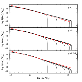
Figure 1.: Left panel: IGIMFs for different cluster mass functions. Upper panel: $\beta=1$; central panel: $\beta=2$; lower panel: $\beta=2.35$. In each panel we have considered 7 possible values of SFRs, ranging from $10^{-−4}$ $M_{\odot}\,yr^{-1}$ (lowermost solid lines) to 100 $M_{\odot}\,yr^{-1}$ (uppermost solid lines), equally spaced in logarithm. Right panel: the open circles are the “fitness” as a function of $\beta$ for various models with different SF efficiencies (indicated by the numbers beside each open circle in units of Gyr^-1.). The horizontal line indicates the fitness value computed for the standard model.

Table 1.: Solar neighbourhood observables, parameters to which they are most sensititve and references.

Observable	Parameter	Reference
SFR Surface density	SF efficency	Rana (1991)
type Ia SNR	Integrated SF history, IMF	Cappellaro (1996)
type II SNR	SF efficiency, IMF	Cappellaro (1996)
Gas surface density	SF efficiency, IMF	Kulkarni & Heiles (1987)
		Olling & Merrifield (2001)
Stellar surface density	SF history, IMF	Weber & de Boer (2009)
Stellar abundance ratios	SF history, IMF	various authors
Stellar Metallicity distribution	SF history, IMF	Jorgensen (2000)
Present-day mass function	SF history, IMF	Miller & Scalo (1979)

2 The (integrated galactic) initial mass function

The main equation used to calculate the IGIMF is (see the contributions by Pflamm-Altenburg et al. and Weidner et al.):

$$\xi_{\rm IGIMF}(m;{\psi}(t))=\int_{M_{\rm ecl,min}}^{M_{\rm ecl,max}({\psi}(t))}\xi(m\leq m_{\rm max})\xi_{\rm ecl}(M_{\rm ecl})dM_{\rm ecl},$$ (1)

where $\psi$ is the star formation rate (SFR). The canonical stellar IMF is $\xi(m)=km^{-\alpha}$, with $\alpha=1.3$ for 0.1 M${}_{\odot}\leq$ $m$ $<$ 0.5 M_⊙ and $\alpha=2.35$ for 0.5 M${}_{\odot}\leq$ $m$ $<m_{\rm max}$. The upper mass $m_{\rm max}$ is a function of the mass of the embedded cluster $M_{\rm ecl}$: this is logical if one considers that small clusters do not have enough mass to produce very massive stars. Star clusters are also apparently distributed according to a single-slope power law, $\xi_{\rm ecl}\propto M_{\rm ecl}^{-\beta}$ (Lada & Lada 2003). In this work we have assumed 3 possible values of $\beta$: 1, 2 and 2.35.
$M_{\rm ecl,min}$ and $M_{\rm ecl,max}(\psi(t))$ are the minimum and maximum possible masses of the clusters in a population of clusters, respectively, and $m_{\rm max}=m_{\rm max}(M_{\rm ecl})$. For $M_{\rm ecl,min}$ we take 5 M_⊙ (the mass of a Taurus-Auriga aggregate, which is arguably the smallest star-forming ”cluster” known). The upper mass of the cluster population depends instead on the SFR and that makes the whole IGIMF dependent on $\psi$.
The standard IMF is a two-slope power law, defined in number as:

$$\xi_{std}(m)=\left\{\begin{array}[]{l l}0.19\,\cdot m^{-2.35}&\qquad{\mathrm{if}}\;m<2\,M_{\odot}\\ 0.24\,\cdot m^{-2.70}&\qquad{\mathrm{if}}\;m>2\,M_{\odot},\\ \end{array}\right.$$ (2)

This equation represents a simplified two-slope approximation of the actual Scalo (1986) IMF. The IMF and all the IGIMFs are normalised in mass to unity as the standard IMF:

$$\int m\xi(m)dm=1.$$ (3)

In Fig. 1, we show the IGIMF as a function of the SFR for the three values of $\beta$ considered in this work, compared to our standard IMF. In general, a lower value of $\beta$ implies a flatter IGIMF, and a hence higher relative fraction of stars with masses $m>1M_{\odot}$.

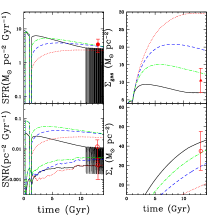
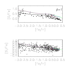
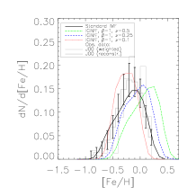
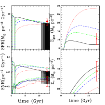
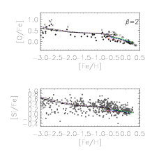
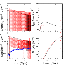
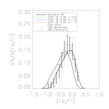
Figure 2.: Upper panels: SFR, type Ia and II SN rates, stellar and gas density versus time (left), abundance ratios (center) and stellar metallicity distribution (right) calculated with $\beta=1$. Middle panels: same as above but with $\beta=2$. Lower panels: same as above but with $\beta=2.35$ (in the left panels only the case with SF efficiency $1.5$ Gyr^-1 is shown). For details see Calura et al. (2010).

3 The chemical evolution model for the Solar Neighbourhood

The main chemical evolution model is described in detail in Calura et al. (2010). The model is calibrated in order to reproduce a large set of observational constraints for the Milky Way galaxy (Chiappini et al. 2001). The Galactic disc is approximated by several independent rings, 2 kpc wide, without exchange of matter between them. The Milky Way is assumed to form as a result of two main infall episodes. During the first episode, the halo and the thick disc are formed. During the second episode, a slower infall of external gas forms the thin disc with the gas accumulating faster in the inner than in the outer region (”inside-out” scenario, Matteucci & François 1989). The process of disc formation is much longer than the halo and bulge formation, with time scales varying from $\sim 2$ Gyr in the inner disc to $\sim 7$ Gyr in the solar region and up to $20$ Gyr in the outermost disc. In this paper, we are interested in the effects of a time-variyng IMF in the Solar Neighbourhood. For this purpose, we focus on a ring located at 8 kpc from the Galactic centre, 2 kpc wide. The model includes the contributions of type Ia SNe, type II SNe and low and intermediate mass stars to the chemical enrichment of the ISM. A SF threshold is adopted ($\sigma_{th}\sim 7M_{\odot}pc^{-2}$) to reproduce various local features, including abundance gradients (Colavitti et al. 2009). The IGIMF is allowed to vary as a function of the SFR, which in turn is a function of cosmic time. The IGIMF is calculated as a function of the SFR according to Eq. 1. In Table  1 we show the solar neighbourhood observables used in this paper, with the main parameters on which they depend and references.
In order to quantitatively compare our results with the observables considered in this paper, we define the $fitness$ quantity as:

$$fitness={1\over{1+\delta}}~{}~{};~{}~{}\delta=\Sigma_{i}{w(i)[{\rm obs}(i)-{\rm theo}(i)]^{2}\over\max\bigl{\{}[{\rm obs}(i)]^{2},[{\rm theo}(i)]^{2}\bigr{\}}}$$ (4)

where, for the $i$-th value of each considered parameter, obs ($i$) and theo ($i$) are the observed values and the predictions of the model, respectively. The weight $w(i)$ is used to give each set of observables the same statistical weight.
The closer $fitness$ is to 1, the better the model is in reproducing the observations. In the right panel of Fig. 1, we show the “fitness” as a function of $\beta$ for all the models considered in this paper (see Sect. 4).

4 Results

Some results of our study are summarized in Fig. 2. Here we show the results of the comparison between observables and model predictions computed with different assumptions for the cluster mass function index $\beta$. In general, the local observed quantities are plotted with their error bars. For a given value of $\beta$, the curves of different types are the model results computed with different assumptions for the SF effiency, reported in the legends. From the time evolution of the SFR, type Ia and II supernova rate (SNR), gas and stellar mass density (left panels) computed with various assumptions for the parameter $\beta$, we can see that lower values of $\beta$ imply higher SNRs, higher gas mass densities and in general lower mass locked up in living stars and remnants. This is visible from the comparison of the results computed with the same values for the SF efficiencies and different values for $\beta$. Another important issue regards the dependence on the star formation threshold: some values of $\beta$ ($\beta=1$, $\beta=2$) show SF histories indendent from the SF threshold. This is basically due to the large mass returned by dying stars, which maintains the gas density always above the threshold level and which produces SF histories substantially different from those obtained with the standard IMF, for which the effect of the threshold is remarkable, in particualr in the last 4 Gyr of evolution. On the other hand, the case with $\beta=2.35$ shows a dependence on the SF threshold even larger than the standard case, and this is due to the lower mass ejection rates from dying stars which stem from a steeper IGIMF (see Fig.  1).
In the middle panel, we show the abundance pattern predicted for the three values of $\beta$, compared to those predicted in the standard case. The elements studied here are O,Si and Fe, since the theoretical understanding of their production is quite clear, and their study allows us to neglect uncertainties related to their nucleosynthesis. In general, lower values of $\beta$ produce higher [Fe/H] values and higher [$\alpha$/Fe] values (i.e. more $\alpha$-enhanced elemental abundances) at a given metallicity. This is related to the fact that the fraction of massive stars increases with decreasing $\beta$ and considering that massive stars are the main producers of $\alpha$ elements. Similar conclusions can be drawn by looking at the plots of the stellar metallicity distributions: the larger the value of $\beta$, the larger the relative fraction of stars producing Fe, i.e. mostly type Ia SNe, i.e. stars in binary systems with initial mass ranging from $0.8M_{\odot}$ to $8M_{\odot}$, hence larger the Fe abundances at any given epoch. This translates in SMDs peaking at higher [Fe/H] values for lower values of $\beta$, assuming the same SF efficiency.
As can be seen from the right panel of Fig. 1, the model calculated with the IGIMF providing the best results is the one with $\beta=2$ and SF efficiency 0.3-0.5 Gyr^-1. The results obtained with this choice of $\beta$ are quite similar to the ones achieved with the standard IMF. This should not be a surprise since, as shown in Fig. 1, in the intermediate case with $\beta=2$ the IGIMF is very similar to the standard IMF. The assumption of $\beta=2$ allows us to satisfactorily reproduce the set of observational constraints considered in this work. This is an important result, given the fact that the IGIMF is computed from first principles. On the basis of the results described in this section, it may be difficut to discriminate between the scenario with the standard IMF and the IGIMF with $\beta=2$. In the next section, the use of a diagnostic possibly useful to disentangle between the standard IMF and the IGIMF will be discussed.

5 Discussion

In this paper, We have modelled the physical properties of the S. N. within the IGIMF theory. In this scenario, the IGIMF can be calculated by combining the cluster mass function with the stellar IMF, which represents the mass function of stars born within clusters and which can be described by a double-slope power law. An important feature of the IGIMF is that it depends on the star formation rate, which in turn evolves with time.

The parameter $\beta$ regulating the cluster mass function may have an important impact on the predicted properties of the Solar Neighbourhood. In general alower value for $\beta$ corresponds to a flatter IGIMF. In terms of chemical evolution, a flatter IGIMF translates into higher mass ejection rates from dying stars, hence globally a lower mass fraction incorporated into stellar remnants and higher gas mass densities. This implies that the evolution of all the models computed assuming $\beta=1$ and $\beta=2$ are not sensitive to the star formation threshold and the star formation histories do not exhibit the “gasping” features typical of the standard model, which in turn is dominated by threshold effects at evolutionary times greater than 10 Gyr. Moreover, the lower the value of $\beta$, the higher the SN rate, the higher the metallicity and the larger the $\alpha$-enhancement visible in the abundance pattern. The statistical test used to compare model results and the obervables indicates that the model which best reproduces the local observables is carachterized by $\beta=2$ as the index of the CMF. The results of the best model are very similar to those obtained with the standard case. A possible diagnostic which could help us disentangling between the two is represented by the present-day mass function (PDMF). The PDMF represents the mass function of living stars as observed in the solar neighbourhood. This quantity is an important diagnostic since it provides pieces of information complementary to the ones from the previously discussed observables.

In the left panel of Fig. 3, we show the PDMF observed in the S. N. and predicted by means of our models. The PDMF computed with the standard IMF agrees with the observations in the range 0.4 $M_{\odot}$ - 2 $M_{\odot}$. At very low stellar masses, the standard IMF seems too steep, whereas the distribution of stars with masses $>30M_{\odot}$ is underestimated. Once again, this is due to the SF threshold, which has strong effects on the SF history of the solar neighbourhood at late times, inhibiting recent SF and hence causing the underabundance or absence of very massive stars. In contrast, the models calculated with the IGIMF provide all similarly a very good fit to the observed PDMF.
The analysis of Fig. 3 seems to suggest that the SF threshold should not play a dominant role in the late evolution of the S. N. Within the IGIMF theory, the existence of a SF threshold may be an observational selection effect, naturally explained in this context as shown by Pflamm-Altenburg et al. (these proceedings). However, as shown by chemical evolution results, the SF threshold is fundamental in reproducing the metallicity gradients observed in the MW and in local galaxies, unless a variable star formation efficiency through the disc is assumed (Colavitti et al. 2009). The study of the abundance gradients within the IGIMF theory may be of crucial help in sheding light on this issue and will be considered in future work.
Another important issue concerns the time evolution of the IGIMF. In the right panel of Fig. 3, we show how the IGIMF varies as a function of time in the case of the three best models computed with different values of $\beta$. The best model ($\beta=2$) shows very small variation of the IGIMF with cosmic time. Strong variations are predicted by assuming $\beta=2.35$, since in this case the star formation history is very much influenced by the effects of the SF threshold. It may be interesting to test the effects of the IGIMF in spiral, Milky Way-like galaxies in a cosmological context. Cosmological semianalytical models predic strong variations in the star formation histories of spiral galaxies (Calura & Menci 2009), which present a large number of spikes due to merging events and which should manifest into strong variations of the IGIMF with redshift.
The universality of the IGIMF is another issue that deserves particular attention in the future. A chemical evolution study of elliptical galaxies within the IGIMF theory shows that the best value for $\beta$ is 2.35, allowing to reproduce best the integrated $\alpha/Fe$ ratios observed in the local early-type galaxies. This value is in contrast with the best value suggested by the analysis of the S. N. features. A further study of the IGIMF in local dwarf irregular galaxies and dwarf spheroidals could certainly be of some help in this regard.
Currently, the slope of the IGIMF in extreme SF conditions is another largely debated topic. Various indirect indications in external galaxies (Dabringhausen, these proceedings) and in our Galaxy (Stolte, these proceedings) seem to suggest that in strongly star forming systems, the slope of the stellar IMF should be flatter than the Salpeter one. Moreover, the assumption of a slightly top-heavy IMF in starbursts helps alleviating the discrepancy between cosmological models and observations regarding the $\alpha/Fe$-$\sigma$ relation observed in local ellipticals (Calura & Menci 2009). Addressing this subject within the IGIMF theory will be of primary importance in the nearest future.

Acknowledgments

FC would like to thank the S.O.C. for the kind invitation and for the financial support, whereas the L.O.C. is acknowledged for being able to establish a pleasant and comfortable environment to discuss exciting scientific topics.

Figure 3.: Left panel: present-day mass function as predicted by means of our models compared to local observations. Right panel: time evolution of the IGIMF assuming various values for the parameter $\beta$.

References

- Bell & Kennicutt (2001) Calura, F., Menci, N., 2009, MNRAS, 400, 1347
- Bell & Kennicutt (2001) Calura, F., Pipino, A., Chiappini, C., Matteucci, F., Maiolino, R., 2009, A&A, 504, 373
- Bell & Kennicutt (2001) Calura, F., Recchi, S., Matteucci, F., Kroupa, P., 2010, MNRAS, 406, 1985
- Bell & Kennicutt (2001) Chiappini, C., Matteucci, F., Romano, D., 2001, ApJ, 554, 1044
- Bell & Kennicutt (2001) Cappellaro, E., 1996, in, eds, Proc. IAU Symp. 171, New Light on Galaxy Evolution. Kluwer Academic, Dordrecht, p.81
- Bell & Kennicutt (2001) Colavitti, E., Cescutti, G., Matteucci, F., Murante, G. 2009, A&A, 496, 429
- Bell & Kennicutt (2001) Elmegreen, B. G., Scalo, J., 2006, ApJ, 636, 149
- Bell & Kennicutt (2001) Kulkarni, S. R., Heiles, C. 1987, in Interstellar Processes, ed. D. Hollenbach, H. Thronson (Dordrecht: Kluwer), 87
- Bell & Kennicutt (2001) Lada, C. J., Lada, E. A. 2003, ARA&A, 41, 57
- Bell & Kennicutt (2001) Matteucci, F., 2001, ASSL Vol. 253, The Chemical Evolution of the Galaxy. Kluwer, Dordrecht, 293
- Bell & Kennicutt (2001) Matteucci, F., François P., 1989, MNRAS, 239, 885
- Bell & Kennicutt (2001) Miller, G. E., Scalo, J. M., 1979, ApJS, 41, 513
- Bell & Kennicutt (2001) Olling, R. P., Merrifield, M. R., 2001, MNRAS, 326, 164
- Bell & Kennicutt (2001) Rana, N. 1991, ARA&A, 29, 129
- Bell & Kennicutt (2001) Recchi, S., Calura, F., Kroupa, P., 2009, A&A, 499, 711
- Bell & Kennicutt (2001) Scalo, J. M., 1986, FCPh, 11, 1
- Bell & Kennicutt (2001) Weber, M., de Boer, W., 2010, A&A, 509, 25
- Bell & Kennicutt (2001) Weidner, C., Kroupa, P. 2006, MNRAS, 365, 1333