Fourth generation quark mass limits in CKM-element space

Abstract

We present a reanalysis of CDF data to extend limits on individual fourth-generation quark masses from particular flavor-mixing rates to the entire space of possible mixing values. Measurements from CDF have set individual limits on masses, $m_{b}^{\prime}$ and $m_{t}^{\prime}$, at the level of $335$–$385$ GeV assuming specific and favorable flavor-mixing rates. We consider the space of possible values for the mixing rates and find that the CDF data imply limits of $290$ GeV and greater over a wide range of mixing scenarios. We also analyze the limits from the perspective of a four-generation CKM matrix. We find that present experimental constraints on CKM elements do not suggest further constraints on fourth-generation quark masses.

I Introduction

A simple modification of the standard model is the addition of a fourth sequential generation of fermion doublets. This natural extension of the standard model reviews may trigger dynamical electroweak symmetry breaking DEWSB without a Higgs boson, and so address the hierarchy problem. The new heavy fermions may have Yukawa couplings so large that they become strong. The subsequent strong dynamics may lead to a composite of fourth generation fermions performing the role of the Higgs hung ; hashimoto1 ; hashimoto2 .

Recent searches by the CDF Collaboration for direct production of the fourth generation quarks, denoted $t^{\prime}$ and $b^{\prime}$ for the up- and down-type, found $m_{t^{\prime}}>335$ GeVCDFt and $m_{b^{\prime}}>385$ GeV CDFb2 , assuming $\mathcal{B}(t^{\prime}\rightarrow W\{q=d,s,b\})=100$% and $\mathcal{B}(b^{\prime}\rightarrow Wt)=100$% respectively. This suggests that fourth generation fermions must indeed be heavy, in support of the compositeness scenario. These searches typically have been interpreted under the assumptions of $m_{t^{\prime}}-m_{b^{\prime}}<M_{W}$ and negligible mixing of the $(t^{\prime},b^{\prime})$ states with the two lightest quark generations. Such conditions are generally required for the SM4 with one Higgs doublet, to account for EW precision data EWPD .

Moreover, when a fourth generation of fermions is embedded in theories beyond the SM, the large splitting case ($m_{t^{\prime}}-m_{b^{\prime}}>M_{W}$) and the inverted scenario ($m_{t^{\prime}}<m_{b^{\prime}}$) have not been excluded. An example of this was given recently hashimoto2 , showing that precision EW data can accomodate $m_{t^{\prime}}-m_{b^{\prime}}>M_{W}$ if there are two Higgs doublets. In fact, the compositeness picture emerging from the addition of new heavy fermionic degrees of freedom is more naturally described at low energies by multi-Higgs theories hung ; hashimoto1 ; hashimoto2 .

This subtle theoretical landscape suggests that there is no uniquely interesting set of assumptions under which experimental data must be interpreted. From the experimental view point, choosing a simple set of assumptions allows straightforward, if narrow, interpretation of results. Yet these interpretations may be extendedlim_prl to give broader and more general results. This article continues the work of our previous Letter lim_prl ; we again consider the possible 4th generation flavor-mixing space broadly, and apply results of the previous searches by CDF to calculate direct limits for arbitrary mixing values and for both cases of $|m_{t^{\prime}}-m_{b^{\prime}}|>M_{W}$. This article includes significant unpublished details of the previous calculations, an additional recently published third dataset CDFb2 , and a translation of the mass limits that we derive in branching fraction space into mass limits in flavor mixing space, which allows for direct comparison with other experimental flavor mixing constraints.

The following sections describe the original CDF measurements, mass limits in branching fraction space, and the limits remapped to CKM4 space.

II Samples and Strategy

The CDF Collaboration has published several important limits on fourth-generation quark masses. We orient this discussion with a summary of their samples and results. Three analyses have been presented: (1) a collection of events containing at least four jets and a single lepton, known as the $\ell+4j$ sampleCDFt ; and (2) a collection of events containing a single lepton, and at least five jets (one with a flavor tag), known as the $\ell+5j$ sampleCDFb2 ; and (3) a collection of events containing two same-charge leptons, two jets (one with a flavor tag) and evidence of neutrinos (missing transverse energy), known as the $\ell^{\pm}\ell^{\pm}jb{\not\!\!E_{T}}$ sample CDFb .

II.1 The $\ell+4j$ sample

In 4.6$\mbox{\,fb}^{-1}$ of data, CDF searched for $t^{\prime}\rightarrow W\{q=d,s,b\}$ decays in the mode

$$p\bar{p}\rightarrow t^{\prime}\bar{t^{\prime}}\rightarrow(W\rightarrow l\nu)q(W\rightarrow qq^{\prime})q$$

by requiring a single lepton and at least four jets. The data were analyzed by reconstructing the invariant mass of the candidate $t^{\prime}$ and measuring the total energy in the event. The event selection used the four jets of highest transverse energy in the event, but did not require a flavor signature ($b$-tag) on any of the jets, making it generally sensitive to $t^{\prime}\rightarrow W\{q=d,s,b\}$. Assuming $\mathcal{B}(t^{\prime}\rightarrow W\{q=d,s,b\})=100\%$, CDF found $m_{t}^{\prime}>335$ GeV.

The mass reconstruction used minimum-likelihood fitting methods that depend upon the particular spectra of final state components. If, for example, one half of an event decayed as $t^{\prime}\rightarrow W(b^{\prime}\rightarrow Wq)$ giving a $WWqWq$ topology (rather than $t^{\prime}\rightarrow Wq$ giving the $WqWq$ topology), it might satisfy the $\ell+4j$ selection criteria, but the reconstructed mass distribution for such events would be significantly modified by the additional $W$. Thus, the results cannot be trivially applied to topologies other than $WqWq$, even when they are expected contributors to the studied sample. We therefore apply the $\ell+4j$ results to $WqWq$ processes exclusively.

II.2 The $\ell+5j$ sample

In 4.8fb^-1 of data, CDF searched for $b^{\prime}\rightarrow Wt$ decays in the mode

$$p\bar{p}\rightarrow b^{\prime}\bar{b^{\prime}}\rightarrow WtW\bar{t} \rightarrow WWbWW\bar{b}$$

$$\rightarrow (\ell^{\pm}\nu)(qq^{\prime})b(qq^{\prime})(qq^{\prime})\bar{b}$$

by requiring at least one lepton, at least five jets (one with a $b$ flavor tag), and missing transverse energy of at least 20 GeV. The data were analyzed by examining the number of jets in the event and the total scalar transverse energy in the event ($H_{T}$). Assuming $\mathcal{B}(b^{\prime}\rightarrow Wt)=100\%$, CDF found $m_{b}^{\prime}>385$ GeV with this signature, the highest limit to date.

As in the $\ell+4j$ sample, the analysis uses minimum-likelihood fitting methods which requires knowledge of the distribution of the signal and background in the $H_{T}$ variable as well as jet multiplicity. Reinterpretting these results to set limits on mixtures of $b^{\prime}\rightarrow Wt$ and $t^{\prime}\rightarrow Wb^{\prime}$ is not possible without knowledge of these distrubutions, so we apply the $\ell+5j$ results exclusively to the $WtWt$ processes.

II.3 The $\ell^{\pm}\ell^{\pm}jb{\not\!\!E_{T}}$ Sample

CDF also searched for $b^{\prime}\rightarrow Wt$ decays in 2.7$\mbox{\,fb}^{-1}$ of data, in the same-charge lepton mode

$$p\bar{p}\rightarrow b^{\prime}\bar{b^{\prime}}\rightarrow WtW\bar{t} \rightarrow WWbWW\bar{b}$$

$$\rightarrow (\ell^{\pm}\nu)(qq^{\prime})b(qq^{\prime})(\ell^{\pm}\nu)\bar{b}$$

by requiring two same-charge leptons, at least two jets (at least one with a $b$-tag), and missing transverse energy of at least 20 GeV.

Given the small backgrounds, multiple neutrinos and large jet multiplicity in the sample, CDF did not reconstruct the $b^{\prime}$ mass, but instead fit the observed jet multiplicity to signal and background templates generated from simulations. Assuming $\mathcal{B}(b^{\prime}\rightarrow Wt)=100\%$, CDF found $m_{b}^{\prime}>338$ GeV.

Since the $\ell^{\pm}\ell^{\pm}jb{\not\!\!E_{T}}$ analysis did not use final-state dependent fits, these results are process independent—they may be applied to any process producing the $\ell^{\pm}\ell^{\pm}jb{\not\!\!E_{T}}$ signal. For example, $t^{\prime}\rightarrow Wb^{\prime}\rightarrow WWt\rightarrow WWWb$ decays would produce a six-$W$, two-$b$ signature, with higher jet multiplicity and larger acceptance to the $\ell^{\pm}\ell^{\pm}jb{\not\!\!E_{T}}$ sample than the simple four-$W$, two-$b$ signature. In this analysis, we therefore apply the $\ell^{\pm}\ell^{\pm}jb{\not\!\!E_{T}}$ results to four-$W$, two-$b$ processes inclusively.

II.4 Analytic Extension of the CDF Results

The three data samples can be seen as probing a region of a two-dimensional interval in branching fraction space which, for the classical splitting ($t^{\prime}$ heavier than $b^{\prime}$), is specified in the following way.

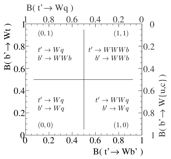
Figure 1: The flavor-mixing interval overlaid with a table of the processes contributing to the corner points

The topologies of $b^{\prime}$ and $t^{\prime}$ decays are determined by four branching fractions, two of which are independent:

$$\mathcal{B}(t^{\prime}\rightarrow Wb^{\prime}) = 1-\mathcal{B}(t^{\prime}\rightarrow W\{q=d,s,b\})$$

$$\mathcal{B}(b^{\prime}\rightarrow Wt) = 1-\mathcal{B}(b^{\prime}\rightarrow W\{q=u,c\})$$

The dependence among these quantities, and the processes they represent, is shown in Fig. 1. In this representation, the $\ell+4j$ analysis, $\ell^{\pm}\ell^{\pm}jb{\not\!\!E_{T}}$ and $\ell+5j$ analyses probe the corner $(0,1)$. Each used the assumption of an individual contribution from one flavor of fourth-generation quark.

We consider the implications of the CDF results in flavor-doublet scenarios, characterized by different assumed mass splittings and a continuum flavor-mixing rates. To extend the interpretations of the published results, we use the basic relationship among event yield, cross section and acceptance to reinterpret the observed yield limits under different assumptions. This requires careful estimation of the relative acceptance between the original assumptions, and those of the new interpretation.

III Mass Limits

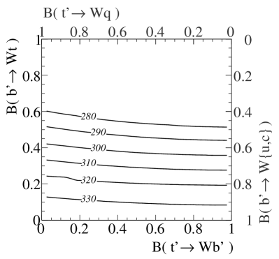
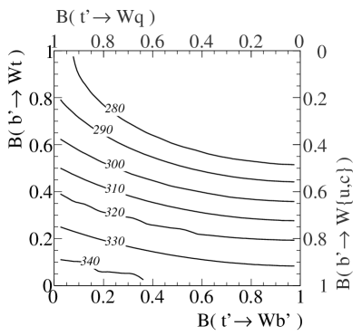
Figure 2: Limits on $b^{\prime}$ mass from $\ell+4j$ data, as a function of branching fractions $\mathcal{B}(t^{\prime}\rightarrow Wb^{\prime})=1-\mathcal{B}(t^{\prime}\rightarrow Wq)$ and $\mathcal{B}(b^{\prime}\rightarrow Wt^{\prime})=1-\mathcal{B}(b^{\prime}\rightarrow Wq)$ for mass structures $m_{t^{\prime}}=m_{b^{\prime}}+100\textrm{GeV}$ (left) and $m_{t^{\prime}}=m_{b^{\prime}}+50\textrm{GeV}$ (right).

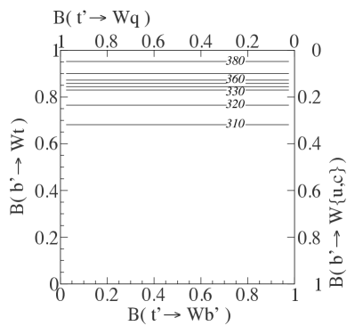
Figure 3: Limits on $b^{\prime}$ mass from $\ell+5j$ data, as a function of branching fractions $\mathcal{B}(t^{\prime}\rightarrow Wb^{\prime})=1-\mathcal{B}(t^{\prime}\rightarrow Wq)$ and $\mathcal{B}(b^{\prime}\rightarrow Wt^{\prime})=1-\mathcal{B}(b^{\prime}\rightarrow Wq)$. The limits do not depend on $m_{t^{\prime}}-m_{b^{\prime}}$ as $t^{\prime}$ gives no contribution.

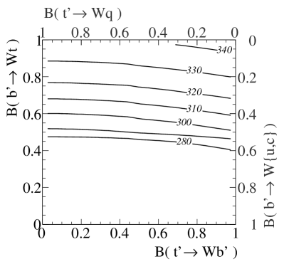
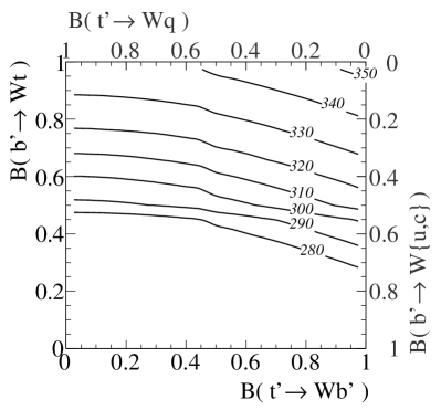
Figure 4: Limits on $b^{\prime}$ mass from $\ell^{\pm}\ell^{\pm}jb{\not\!\!E_{T}}$ data, as a function of branching fractions $\mathcal{B}(t^{\prime}\rightarrow Wb^{\prime})=1-\mathcal{B}(t^{\prime}\rightarrow Wq)$ and $\mathcal{B}(b^{\prime}\rightarrow Wt^{\prime})=1-\mathcal{B}(b^{\prime}\rightarrow Wq)$ for mass structures $m_{t^{\prime}}=m_{b^{\prime}}+100\textrm{GeV}$ (left) and $m_{t^{\prime}}=m_{b^{\prime}}+50\textrm{GeV}$ (right).

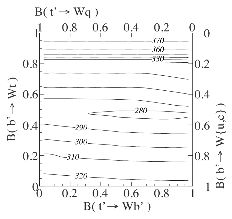
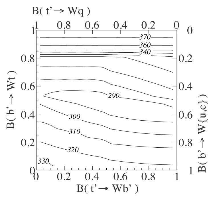
Figure 5: Limits on $b^{\prime}$ mass from $\ell^{\pm}\ell^{\pm}jb{\not\!\!E_{T}}$, $\ell+5j$ and $\ell+4j$ data, as a function of branching fractions $\mathcal{B}(t^{\prime}\rightarrow Wb^{\prime})=1-\mathcal{B}(t^{\prime}\rightarrow Wq)$ and $\mathcal{B}(b^{\prime}\rightarrow Wt^{\prime})=1-\mathcal{B}(b^{\prime}\rightarrow Wq)$ for mass structures $m_{t^{\prime}}=m_{b^{\prime}}+100\textrm{GeV}$ (top) and $m_{t^{\prime}}=m_{b^{\prime}}+50\textrm{GeV}$ (bottom).

In general, the event yield divided by the integrated luminosity, $N/L$, is equal to the cross section times the acceptance rate. For a particular process, such as individual $b^{\prime}$, this simply tells us that the limit on a cross section, given an observed yield limit, is given by

$$\sigma_{b^{\prime}}=\frac{N}{L\cdot\epsilon_{b^{\prime}}}\textrm{,}$$ (1)

where $\epsilon_{b^{\prime}}$ is the acceptance rate for the observed process within the experimental selection constraints. However, we can also consider the case with two contributions if we know the relative acceptance rates between the processes, $\epsilon_{rel}$, and if the two cross sections are dependent:

$$\frac{N}{(L\cdot\epsilon_{b^{\prime}})}=\sigma_{b^{\prime}}+\epsilon_{rel}\cdot\sigma_{t^{\prime}}(\footnotesize\sigma_{b^{\prime}}).$$ (2)

Here, the dependence of the $t^{\prime}$ cross section on the $b^{\prime}$ cross section is given, from the next-to-leading order cross-section calculations for massive quarksxsnlo , by the mass splitting. Need to add comment on sigma rel!

To probe the full two-dimensional branching fraction interval, we must calculate the dependence of the event yield on the branching fractions explicitly. As the branching fractions to the reconstructed states vary, the acceptances of the processes of interest vary accordingly. Reconstruction efficiencies can differ as well. Considering these effects, we calculate the acceptances of $b^{\prime}$ and $t^{\prime}$ in the $\ell+4j$, $\ell+5j$ and $\ell^{\pm}\ell^{\pm}jb{\not\!\!E_{T}}$ samples.

The expected signal yield for one process relative to another is proportional to relative production rates and final-state reconstruction efficiencies. The relative signal production rates have two factors: the relative cross section for initial state production and the branching ratios of the involved processes (second-order when both sides of the event are considered, as here). When several processes contribute to a signal there are multiple terms of this form. Fixing the event yield at its observed value, we may isolate the cross section we wish to limit, and express it in terms of the previously measured limit and an effective relative acceptance. The effective relative acceptance $A$ includes acceptance terms for all processes considered, each scaled by relative cross-section.

In the $\ell+4j$ case, there are no relative reconstruction efficiencies to consider, and we have a simple expression for the relative expected yields as a function of $\beta_{b^{\prime}}=\mathcal{B}(b^{\prime}\rightarrow Wt)$ and $\beta_{t^{\prime}}=\mathcal{B}(t^{\prime}\rightarrow Wb^{\prime})$:

$$A(\beta_{b^{\prime}},\beta_{t^{\prime}})=(1-\beta_{b^{\prime}})^{2}+\sigma_{rel}(1-\beta_{t^{\prime}})^{2}$$ (3)

We use this expression to produce limits on the mass of the $b^{\prime}$ as a function of fourth-generation branching fractions. The results, shown in the interval introduced before, are presented in Fig. 2.

The $\ell+5j$ case is similar, as we are limited in our reinterpretation of the published results, and can only write

$$A(\beta_{b^{\prime}},\beta_{t^{\prime}})=\beta_{b^{\prime}}^{2}$$ (4)

with the limits shown in Fig. 3.

The $\ell^{\pm}\ell^{\pm}jb{\not\!\!E_{T}}$ case is somewhat more complicated. In addition to $b^{\prime}$, there are two significant $t^{\prime}$ processes that produce the signal selected for the sample analyzed:

$$t^{\prime}\rightarrow Wb^{\prime} \rightarrow WWt\rightarrow WWWb$$

$$t^{\prime}\rightarrow Wb^{\prime} \rightarrow WWc$$

Moreover, because of jet multiplicity and the flavor-tag requirement, it is necessary to consider relative reconstruction efficiencies for each contribution. These factors are denoted $\epsilon_{NW}$, where $N$ is the number of intermediate $W$-bosons in the process described. Presented in Table 1, they are estimated from simulated data and are calculated relative to the four-$W$ case considered in the original analysis.

$$A(\beta_{b^{\prime}},\beta_{t^{\prime}})=\beta_{b^{\prime}}^{2}+\beta_{t^{\prime}}^{2}\frac{\sigma_{rel}}{\epsilon_{bb}}[(1-\beta_{b^{\prime}})^{2}\epsilon_{4W}\epsilon_{cc}$$ (5)

$$+ 2\beta_{b^{\prime}}(1-\beta_{b^{\prime}})\epsilon_{5W}\epsilon_{cb}+\beta_{b^{\prime}}^{2}\epsilon_{6W}\epsilon_{bb}]$$

The different terms in the $t^{\prime}$ contribution have different reconstruction efficiencies due to jet-flavor tagging, expressed by $\epsilon_{f_{1}f_{2}}$ where $f_{1}f_{2}$ is the flavor combination of the quarks in the final state of the quark-level $t^{\prime}$ decay. These efficiencies are given by statistics from the raw efficiencies of the jet-flavor tag to select the beauty (60%) or charm (15%) flavor in a jet:

$$\epsilon_{bb} = 1-(1-\epsilon_{b})^{2}$$

$$\epsilon_{cb} = \epsilon_{c}(1-\epsilon_{b})+\epsilon_{b}(1-\epsilon_{c})+\epsilon_{b}\epsilon_{c}$$

$$\epsilon_{cc} = 1-(1-\epsilon_{c})^{2}$$

Again, we produce limits on the mass of the $b^{\prime}$ as a function of fourth-generation branching fractions. The results are presented in Fig. 4.

As expected, inspection of these results reveals the complementary sensitivities of the CDF analyses. However, they are not orthogonal and thus cannot be statistically combined. In view of this, we produce the best limits over the branching fraction interval by choosing the stronger of two limits at each point. The combined results are presented in Fig. 5.

Table 1: Reconstruction efficiencies for $t^{\prime}$ decays mediated by W bosons, relative to the $b^{\prime}$ reconstruction efficiency of the original CDF analysis.

$m_{t^{\prime}}-m_{b^{\prime}}$	50GeV	100GeV
$\epsilon_{4W}$	0.63	0.86
$\epsilon_{5W}$	1.07	1.51
$\epsilon_{6W}$	1.60	2.16

IV CKM4 Mapping

To compare results of many different experiments, it is useful to decouple the various physical parameters wherever possible and express the results in terms of the underlying physical quantities at the theoretical level. In this case, these are the elements of the flavor mixing matrix, on which there are important experimental constraints.

The description of SM quark flavor mixing falls to the CKM matrix, which, in the presence of a fourth generation, is extended to CKM4. It has 16 elements parametrized by 4 mixing angles and three irreducible CP-violating phasesckm4 . Present experimental data has been brought to bear on the extent to which this could be consistent with observation (cf. ckm4 ).

The ideal case would be to form a clear basis of comparison between theory and experiment, and some of the challenges of doing that are topics of discussion here. The primary difficulty is in decoupling the many dependent parameters involved, so one aims to formulate analysis to this end. Here, we eliminate many degrees of freedom by treating light quarks as indistinguishable. The scale of light quark mass is relative to the mass difference with $W$, as required for weak decay. This treatment is also natural from the perspective of experimental design.

In the limit of massless particles, the branching fractions of the previous sections translate directly to the squares of the magnitudes of the corresponding CKM4 elements:

$$\mathcal{B}(t^{\prime}\rightarrow Wb^{\prime}) = |V_{t^{\prime}b^{\prime}}|^{2}$$

$$\mathcal{B}(b^{\prime}\rightarrow Wt) = |V_{tb^{\prime}}|^{2}$$

In the case of massive particles, the partial widths carry on this proportionality, but there are also phase-space constraints to consider. The branching fraction of the massive particle is of course constructed from the partial widths of the various possible modes. Thus the branching fraction has dependence on the masses of the parent and daughter particles.

This presents a challenge: can we discuss fourth generation mass limits in the context of a CKM parametrization? Ignoring for the moment the issue of mass dependance, we can construct a transformation between the branching fractions and the CKM elements.

The plane we have chosen, with axes $\mathcal{B}(t^{\prime}\rightarrow Wb^{\prime})=1-\mathcal{B}(t^{\prime}\rightarrow Wq)$ [$q=d,s,b$] and $\mathcal{B}(b^{\prime}\rightarrow Wt)=1-\mathcal{B}(b^{\prime}\rightarrow Wq)$ [$q=u,c$] includes processes with tree-level diagrams having vertex factors of $V_{44}$ and $V_{34}$ respectively. Of course, a branching fraction is the quotient ${\Gamma_{\textrm{partial}}}/{\Gamma_{\textrm{total}}}$.

At tree-level, the partial widths of the final states are the product of phase-space and weak-coupling factors, and the absolute square of the tree-level CKM vertex factor.

For the total widths of the denominators, we would like to eliminate dependence on the mixing angles between the fourth generation and the lighter quarks to minimize the number of variables involved in the transformation. At tree-level, this seems again possible:

1. The phase-space factors of matrix elements to the various flavors are nearly identical for all light quarks, including $b$ when the mother quark is a $t^{\prime}$.

2. By weak universality we can eliminate the CKM parameters that describe the mixing with lighter quarks.

IV.1 $\mathcal{B}(t^{\prime}\rightarrow Wb^{\prime})$ as a function of $V_{44}$

For the numerator:

$$\|V_{44}\|^{2}\cdot\|\int^{(t^{\prime},b^{\prime})}dp^{4}(...)\|^{2}$$

The integral over four-space is meant to signify the full matrix element for the process indicated by superscript, excluding only the CKM factor. The matrix element is calculated using the software program BRI BRI , in a configuration that models no quark mixing (to decouple the CKM suppression).

For the denominator, we have such a term for each generation:

$$\|V_{41}\|^{2}\cdot\|\int^{(t^{\prime},d)}dp^{4}(...)\|^{2}+\|V_{42}\|^{2}\cdot\|\int^{(t^{\prime},s)}dp^{4}(...)\|^{2}$$

$$+\|V_{43}\|^{2}\cdot\|\int^{(t^{\prime},b)}dp^{4}(...)\|^{2}+\|V_{44}\|^{2}\cdot\|\int^{(t^{\prime},b^{\prime})}dp^{4}(...)\|^{2}$$

$$=\{\|V_{41}\|^{2}+\|V_{42}\|^{2}+\|V_{43}\|^{2}\}\cdot\|\int^{(t^{\prime},q)}dp^{4}(...)\|^{2}$$

$$+\|V_{44}\|^{2}\cdot\|\int^{(t^{\prime},b^{\prime})}dp^{4}(...)\|^{2}$$

$$=\{1-\|V_{44}\|^{2}\}\cdot\|\int^{(t^{\prime},q)}dp^{4}(...)\|^{2}$$

$$+\|V_{44}\|^{2}\cdot\|\int^{(t^{\prime},b^{\prime})}dp^{4}(...)\|^{2}$$

In the case of the branching fraction for unmixed weak fourth-generation decay, we obtain a simple transformation between the branching fraction and the corresponding CKM vertex factor.

IV.2 $\mathcal{B}(b^{\prime}\rightarrow Wt)$ as a function of $V_{43}$ and $V_{44}$

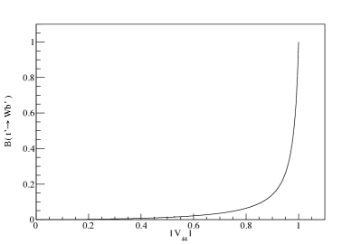
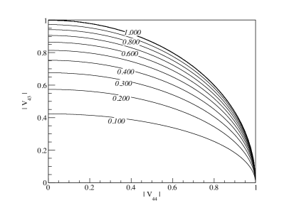
Figure 6: Mapping from branching fraction to CKM4 space for mass structure $m_{t^{\prime}}=m_{b^{\prime}}+100\ \textrm{GeV}$. Left, $\mathcal{B}(t^{\prime}\rightarrow Wb^{\prime})$ as a function of CKM4 parameters $V_{44}$. Right, $\mathcal{B}(b^{\prime}\rightarrow Wt)$ as a function of $V_{43}$ and $V_{44}$.

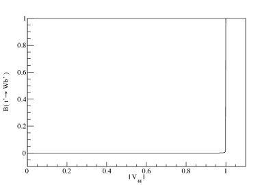
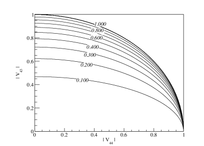
Figure 7: Mapping from branching fraction to CKM4 space for mass structure $m_{t^{\prime}}=m_{b^{\prime}}+50\ \textrm{GeV}$. Left, $\mathcal{B}(t^{\prime}\rightarrow Wb^{\prime})$ as a function of CKM4 parameters $V_{43}$ and $V_{44}$. Right, $\mathcal{B}(b^{\prime}\rightarrow Wt)$.

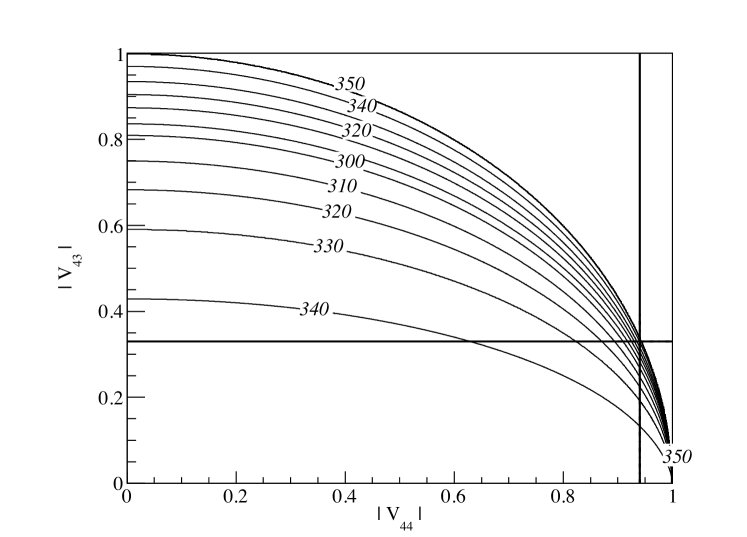
Figure 8: Limits on $b^{\prime}$ mass from $\ell^{\pm}\ell^{\pm}jb{\not\!\!E_{T}}$, $\ell+5j$ and $\ell+4j$ data, as a function of CKM4 parameters $V_{43}$ and $V_{44}$ for mass structures $m_{t^{\prime}}=m_{b^{\prime}}+100\ \textrm{GeV}$ (top) and $m_{t^{\prime}}=m_{b^{\prime}}+50\ \textrm{GeV}$ (bottom).

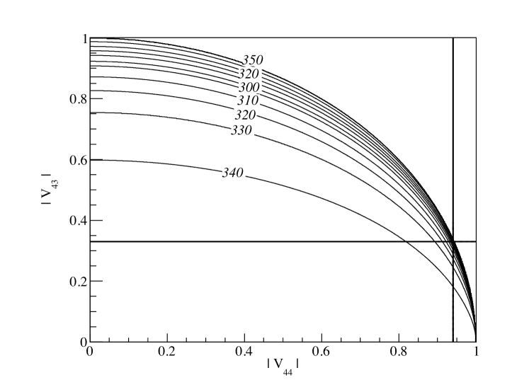
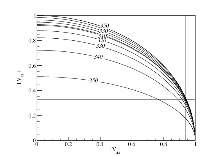
Figure 9: Limits on $b^{\prime}$ mass from $\ell^{\pm}\ell^{\pm}jb{\not\!\!E_{T}}$, $\ell+5j$ and $\ell+4j$ data, as a function of CKM4 parameters $V_{43}$ and $V_{44}$ for mass structures $m_{t^{\prime}}=m_{b^{\prime}}+100\ \textrm{GeV}$ (top) and $m_{t^{\prime}}=m_{b^{\prime}}+50\ \textrm{GeV}$ (bottom) using alternate mappings from branching ratio space with varied phase-space assumptions. Compare to Fig. 8.

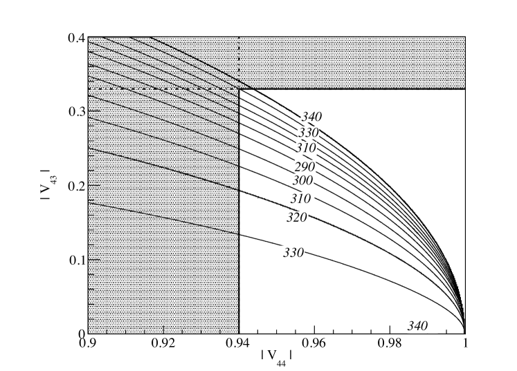
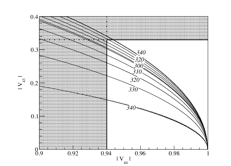
Figure 10: Limits on $b^{\prime}$ mass from $\ell^{\pm}\ell^{\pm}jb{\not\!\!E_{T}}$, $\ell+5j$ and $\ell+4j$ data, as a function of CKM4 parameters $V_{43}$ and $V_{44}$ in the region of interest, for mass structures $m_{t^{\prime}}=m_{b^{\prime}}+100\ \textrm{GeV}$ (top) and $m_{t^{\prime}}=m_{b^{\prime}}+50\ \textrm{GeV}$ (bottom).

For the case when the fourth generation $b^{\prime}$ mixes with the third generation in decay, the situation is slightly more complicated. Here we cannot describe the branching fraction using only the CKM vertex factor $V_{34}$, because the presence of the kinematically inaccessible (assuming classical splitting) $t^{\prime}$ nevertheless affects our expression for the total width when we apply the weak universality constraint to remove the dependence on mixing with the lighter generations.

$$\{1-\|V_{34}\|^{2}-\|V_{44}\|^{2}\}\cdot\|\int^{(b^{\prime},q)}dp^{4}(...)\|^{2}$$

$$+\|V_{34}\|^{2}\cdot\|\int^{(b^{\prime},t)}dp^{4}(...)\|^{2}$$

In this simplified model, the transformation has only two degrees of freedom associated with the phase space integrals. These may be expressed by the ratio of the two factors in each equation. This is expected since we have reduced the structure of the quark masses to two splittings, that between $t^{\prime}$ and $b^{\prime}$, and between $b^{\prime}$ and $t$.

In Fig. 6, we show the branching ratio as a function of the two relevant CKM4 parameters, $V_{43}$ and $V_{44}$ for the mass structure $m_{t^{\prime}}=m_{b^{\prime}}+100\ \textrm{GeV}$. Figure 7 shows the same for $m_{t^{\prime}}=m_{b^{\prime}}+50\ \textrm{GeV}$. Although strictly speaking the $W$ is virtual in this case, its behavior in the decay is essentially indistinguishable from the on-shell case. Finally, we present limits on the fourth generation quarks in the CKM4 space, see Figure 8.

The transformation is sensitive to the phase space assumptions, as the amount of available phase space is mass-dependent. Thus it is important to consider the consistency of this assumption with the limits set. To demonstrate this, we perform the transformation with phase-space assumptions that span the range of limits set. The degree to which the limit contours in CKM space change is a measure of the robustness of the transformation. There is very little change as the mass of the $b^{\prime}$ increases to the the top of the range and beyond. As the $b^{\prime}$ mass is reduced to 300 GeV and below, some appreciable variation occurs. This variation is shown in Fig. 9 . Inspection of the figures shows the transformation to be robust over the interval of limits set by these data.

The region favored by other experimental data is $V_{43}<0.3$ and $V_{44}>0.94$. Figure 10 shows the limits in this region of interest.

V Conclusions

We reiterate the conclusions of our earlier Letterlim_prl : we find that the CDF data imply limits on $m_{b^{\prime}}$ and $m_{t^{\prime}}$ of $290$ GeV and greater over the full range of mixing scenarios, for two characteristic choices of the $t^{\prime}$- $b^{\prime}$ mass splitting: $m_{t^{\prime}}>m_{b^{\prime}}$ and $m_{b^{\prime}}>m_{t^{\prime}}$. The inclusion of a $t^{\prime}$ strengthens the previously obtained $b^{\prime}$ mass limit from the $\ell^{\pm}\ell^{\pm}jb{\not\!\!E_{T}}$ sample; in the $m_{t^{\prime}}>m_{b^{\prime}}$ case, by up to 10% when $0<m_{t^{\prime}}-m_{b^{\prime}}<M_{W}$. Because of its range of sensitivity, the addition of the $\ell+5j$ sample, while increasing the mass limits in some neighborhoods of parameter space, does not significantly improve the overall results of this analysis.

The transformation of the mass limits to CKM space is found to be fairly robust despite the variation in the phase-space description. Based on electroweak CKM limitsckm4 , we can identify a region of branching-fraction parameter space that is most interesting, but this does not further constrain the range of mass limits set by the available data.

VI Acknowledgements

We thank Tim Tait, Shaouly Bar-Shalom and Alexander Lenz for useful conversations. The authors are supported by grants from the Department of Energy Office of Science and by the Alfred P. Sloan Foundation.

References

- (1) P.H. Frampton, P.Q. Hung and M. Sher, Phys. Rept. 330, 263 (2000); B. Holdom, W.S. Hou, T. Hurth, M.L. Mangano, S. Sultansoy, G. Unel, presented at Beyond the 3rd SM generation at the LHC era workshop, Geneva, Switzerland, Sep 2008, arXiv:0904.4698 [hep-ph], published in PMC Phys. A3, 4 (2009).
- (2) B. Holdom, Phys. Rev. Lett. 57, 2496 (1986) [Erratum-ibid. 58, 177 (1987); W.A. Bardeen, C.T. Hill and M. Lindner, Phys. Rev. D41, 1647 (1990); C. Hill, M. Luty and E.A. Paschos, Phys. Rev. D43, 3011 (1991); P.Q. Hung and G. Isidori Phys. Lett. B402, 122 (1997).
- (3) P.Q. Hung and Chi Xiong, arXiv:0911.3890 [hep-ph]; ibid. arXiv:0911.3892 [hep-ph]; H. J. He, C. T. Hill and T. M. P. Tait, Phys. Rev. D 65, 055006 (2002) [arXiv:hep-ph/0108041].
- (4) M. Hashimoto, V.A. Miransky, arXiv:0912.4453 [hep-ph].
- (5) M. Hashimoto, arXiv:1001.4335 [hep-ph].
- (6) A. Lister (for the CDF collaboration), presented at ICHEP 2008, arXiv:0810.3349 [hep-ex]; J. Conway et al., CDF public conference note CDF/PUB/TOP/PUBLIC/10110.
- (7) L. Scodellaro (for the CDF collaboration) presented at ICHEP 2010. D. Whiteson et al., CDF public conference note CDF/PUB/TOP/PUBLIC/10243
- (8) T. Aaltonen et al. (by the CDF Collaboration), arXiv:0912.1057 [hep-ex].
- (9) C.J. Flacco, D. Whiteson, T.M.P. Tait, S. Bar-Shalom, Phys. Rev. Lett. 105, 111801 (2010)
- (10) M. Bobrowski, A. Lenz, J. Riedl, J. Rohrwild, Phys. Rev. D79, 113006 (2009);
- (11) P. Meade, M. Reese, arXiv:hep-ph/0703031v2 [hep/ph]
- (12) G.D. Kribs, T. Plehn, M. Spannowsky, T.M.P. Tait, Phys. Rev. D76, 075016 (2007); ibid. Nucl. Phys. Proc. Suppl. 177-178, 241-245 (2008); M.S. Chanowitz, Phys. Rev. D79, 113008 (2009); V.A. Novikov, A.N. Rozanov and M.I. Vysotsky, arXiv:0904.4570 [hep-ph] and references therein; J. Erler and P. Langacker, arXiv:1003.3211 [hep-ph].
- (13) A. Arhib and W.S. Hou, JHEP 0607, 009 (2006); M. Bobrowski, A. Lenz, J. Riedl and J. Rohrwild, Phys. Rev. D79, 113006 (2009); A. Soni, A.K. Alok, A. Giri, R. Mohanta, S. Nandi, arXiv:0807.1971 [hep-ph]; G. Eilam, B. Melic and J. Trampetic, Phys. Rev. D80, 116003 (2009); A. Soni, A.K. Alok, A. Giri, R. Mohanta, S. Nandi, arXiv:1002.0595 [hep-ph]; A.J. Buras et al., arXiv:1002.2126 [hep-ph].
- (14) R. Bonciani, S. Catani, M. L. Mangano, and P. Nason, Nucl. Phys. B529, 424 (1998). M. Cacciari, S. Frixione, M. L. Mangano, P. Nason, and G. Ridolfi, J. High Energy Phys.04 (2004) 068.
- (15) H. J. He, N. Polonsky and S. f. Su, Phys. Rev. D 64, 053004 (2001) [arXiv:hep-ph/0102144].
- (16) R. Bonciani, S. Catani, M. L. Mangano, and P. Nason, Nucl. Phys. B529, 424 (1998); M. Cacciari, S. Frixione, M. L. Mangano, P. Nason, and G. Ridolfi, J. High Energy Phys. 04 (2004) 068.
- (17) J. Alwall et al., JHEP 0709, 028 (2007) [arXiv:0706.2334 [hep-ph]].
- (18) P. Meade and M. Reece, arXiv:hep-ph/0703031.