Superposition and Entanglement from Quantum Scope

Abstract

The abstract framework of quantum mechanics (QM) causes the well-known weirdness, which leads to the field of foundation of QM. We constructed the new concept, i.e., scope, to lay the foundation of quantum coherence and openness, also the principles of superposition and entanglement. We studied analytically and quantitatively the quantum correlations and information, also we discussed the physical essence of the existed entanglement measures. We compared with several other approaches to the foundation of QM, and we stated that the concept of scope is unique and has not been demonstrated before.

I INTRODUCTION

Quantum mechanics (QM), particularly featured by $\hbar$ and $|\psi\rangle$, has been always facing the fundamental critics since its establishment Bohm ; Jammer ; bell87 . The exact physical meaning of “quantum” is unclear, which leads to the well-known “weirdness”. The development of quantum field theory (QFT), which is often viewed as an improved form of QM, does not resolve the seminal problems in QM, such as the direct physical meaning of wave function and phase, the role of quantization and measurement, etc. The problem of the foundation of QM has been widely concerned again due to the progress of quantum information and quantum computing (QIQC) Nielsen ; zurek03 ; schlosshauer ; Timpson . The concepts of nonlocality and entanglement have proven their importance, yet, there exist confusions between them NE .

For the research of foundation of QM, we can briefly clarify two sub-fields, one is the interpretation of QM epr ; Schrodinger ; bohm52 ; neumann ; everett ; zeh ; ballentine ; pct ; ch ; cramer ; fraassen ; mermin ; Dewdney ; Aharonov ; Aerts ; Ronde ; Jansson , the other is the post-QM Hardy ; Fuchs ; popescu ; Bub ; Gorobey ; Butterfield ; Ashtekar ; Iliev ; Isham07 . The problems and confusions on basic concepts even philosophy, such as the classical zurek03 ; schlosshauer , hidden variable bohm52 , collapse pct , etc are mostly addressed in the interpretations. Post-QM also devotes to the complete mathematical form of QM, such as the information-theoretic approach Bub , the Kähler structure approach Ashtekar , etc.

The standard QM bases on several assumptions, and the physical explanations of the Copenhagen (orthodox) interpretation are not satisfying. Uncertainty and complementarity are emphasized; however, for uncertainty, there are different explanations, either based on measurement, knowledge, propensity, or reality Jammer . For the statistical meaning of the wave function and measurement, the disagreement is more notable. Born viewed statistics as inherent, while Einstein, by EPR-argument epr , viewed statistics as a result of incompleteness of QM. The notable “jump” and “collapse” do not have clear physical pictures. The most primary problem is that the Copenhagen interpretation did not give an exact and direct meaning to the wave function, e.g., why $|\psi\rangle$ is complex?

Indeed, there are direct efforts to explain the physical meaning of wave function, which led to the hidden variable method and Bohm mechanics bohm52 . Every particle is endowed with definite coordinate and trajectory under the restraint of guiding wave. Also, there exists the physical collapse theory aimed to explain collapse pct . However, it modifies the Schrödinger equation and the linearity, which is shown to be the analogy of the approaches based on decoherence schlosshauer . Coherence and decoherence, which were not demonstrated in the standard QM, have gained lots of attentions these years. For instance, the many-world interpretation everett views the universe as a coherent entity, and there exist the inner observer and relative state. The consistent (decohered) history approaches ch take the time evolution and measurement into account, and demonstrate the structure of quantum logic. In Zurek’s exsistential interpretation zurek03 , the uncertainty principle is re-explained from the view of information, and the Born’s rule is deduced via the symmetry of envariance. Recently, kinds of information-theoretic theories Bub are developed, where QM is viewed as a kind of information processing theory. With all these progresses, however, the exact essence of quantum has not been drawn.

At the same time, the continuous argument on foundation of QM also arose the reflection of the primary philosophical conception, which cannot be avoided in the quantum physics. The problem that why we cannot easily understand QM just brings the problem that why we think the classical mechanics (CM) is normal. In this paper, our standing point is to view QM as a special kind of “description” of motion, from which, there is no good or bad of QM and CM bohr . The theories, with equations and models, deal with the same nature only revealing different aspects and properties. The state vector in Hilbert space can capture the properties of coherence, e.g., interference, which is exotic for CM. On the contrary, trajectory is the basic idea in CM and the macroscopic world, yet, not in QM, due to the uncertainty. We note the trajectory in the path-integral method, which borrows ideas from CM, only has mathematical meaning. In practice (reality), to employ which description depends on its efficiency.

In this work, we start from one new concept, “scope”, to check the foundation of QM. We focus on the basic concepts and ideas in QM, mostly relating to superposition. We do not intend to construct a broader theory with the standard QM as the special case, the methods based on scope mainly belong to the interpretation of QM. Scope describes the “structure of motion”, i.e., the logic and systematic potential action region of the movement of a certain object (system). That is, from scope we can get the ability and the whole structure of the motion of the matter. The merits of the concept of scope are multi-folds. Firstly, the direct one, the weirdness of QM can be resolved based on scope, the wave function and superposition can get their physical meaning. Secondly, the abstract QM can gain solid natural foundation and physical essence, i.e., QM is a totally new kind of description different with CM (including statistical mechanics) and also Relativity. Thirdly, scope can bring new ideas. For instance, the wave function and superposition principle can also be used in the mesoscopic and macroscopic scales, that is, the concept of scope is universal, cannot be restricted by the scale. Also, QM may not rely on the Hilbert space, since scope itself can form a kind of space, also there can be other kinds of space, e.g., tangnet wang , relating to quantum information and entanglement. Forth, another point, the concept of scope may have new indication of the basic ideas of nature and philosophy, e.g., it means every object has finite ability of motion.

This work is divided into four parts. In Sec. II, we start from the concept of openness, which is central for QM, to clarify several basic physical ideas. In Sec. III, we introduce the new concept of “scope”, from which we discuss the physical meaning of superposition and entanglement, and to address the foundation of QM. In Sec. IV, we study several kinds of quantum states, and we analyze the degree of entanglement and information. Several topics are discussed in the appendix. One is the differences between scope and other existed methods, where we state that the concept of scope has never been proposed before. Another one is the model for the reduced entanglement, by comparison with the two-body problem in CM. Last, we study the physical meaning of entanglement measures at present, like negativity, relative entropy of entanglement. In Sec. V, we conclude and discuss briefly the physical roles of scope in the foundation of QM.

II OPENNESS

In this section, before the study on the concept of scope and entanglement, we show that the concept of openness is fundamental in QM. Openness means that the quantum object cannot be separated from the outside world, and the basic subject in QM is the open system, just the opposite of CM zeh ; wang . The physical reason for openness is the existence of quantum coherence. We show that all the basic equations in QM demonstrate the openness and coherence.

II.1 Coherence

The quantum coherence leads to many crucial facts, such as the double-slit interference, coherent and squeezed state of light, also the Heisenberg’s uncertainty principle, etc. Relating to measurement, the uncertainty principle states that any measurement disturbs the state of the quantum system, since the coherence is disturbed. On the contrary, the nature light from sun is not coherent as it is a kind of mixture. In CM, there is no coherence, which is the main distinction between quantum and classical dynamics wang . Usually, in QM the method of density matrix Fano is employed to capture coherence, which is represented by the non-diagonal elements. A diagonal density matrix is said to be classical as the coherence vanishes. In QFT, there exists coherence since the quantum field itself is the coherent entity, such as vacuum, electromagnetical field etc, although the density matrix is not often used. “Coherent” means that the field as a whole has fixed amplitude and phase. The micro-particles, as the excited state of field, have coherence since interactions between them are due to the field. The facts of particle creation, classicality, and decoherence lead to the degeneracy of coherence, yet, particle can go back to its ground state via the annihilation operator, thus, re-excite the coherence Calzetta ; Habib .

In addition, we note that the standard QM does not focus on the properties of field, e.g., the creation and vanish of particles, also the origin of ensemble, which we will discuss below.

II.2 Ensemble

In QM, there was the argument that whether quantum theory describes the dynamics of the single system or the ensemble ballentine . According to the standard QM, the existence of ensemble is a priori fact. For instance, in the double-slit interference experiment, the ensemble of electrons is used, the electrons are viewed as identical, and the state of electrons are the superposition of two modes corresponding to the two slits. Here, QM cannot explain the origin of the ensemble; in contrast, QFT can give the creation-annihilation picture of the ensemble of electrons. The quantum states of each electron before entering the slit are not necessarily orthogonal, and there exists field among the electrons, that is, the existence of ensemble does not mean there is no coherence.

Yet, the methods of QM are believed as universal everett , thus, it should provide the physical picture for ensemble. Recently, there are efforts to indicate the quantum origin of ensemble via entanglement Popescu ; Kim . It is shown that the system within the coherent universe behaves as the canonical ensemble, as if the universe were in the mixed state, in which each pure state has the equal probability. Physically, there can be kinds of coherence and decoherence processes in QM, which relates to the distinction between the fine-grained and coarse-grained description of states of the system Calzetta . We will further analyze this in the study of density matrix below. In addition, we note that the concept of ensemble is similar to “mixture”, which is also widely employed in QM. However, the “mixed state” is not an exact expression, e.g., it does not indicate the state is of one single object or many objects. We view mixture as the classical concept.

II.3 Openness

The coherence indicates the openness of quantum dynamics. Here we show that the basic equations of QM all demonstrate the openness. The Schrödinger equation $i\hbar|\dot{\Psi}\rangle=\mathcal{H}|\Psi\rangle$, where $|\Psi\rangle$ is viewed as the pure state vector of the system, from which the eigenstate and the eigen-energy can be deduced. The single quantum system can be, e.g., one electron, field, or ensemble of electrons, as long as there exists coherence. Here, “single” is different with that in CM, where the system is labeled by mass. The wave function has the property of holistic, and we can say that the system is “open inside”. Now, for Schrödinger equation, it is easy to get the following equations

$$i\hbar\dot{|\Psi\rangle}\langle\Psi| = \mathcal{H}|\Psi\rangle\langle\Psi|,$$ (1)

$$-i\hbar|\Psi\rangle\dot{\langle\Psi|} = |\Psi\rangle\langle\Psi|\mathcal{H}^{\dagger},$$

where Hamiltonian $\mathcal{H}=\mathcal{H}^{\dagger}$. Let the density matrix (or statistical matrix) $\rho=|\Psi\rangle\langle\Psi|$, and $\dot{\rho}=\dot{|\Psi\rangle}\langle\Psi|+|\Psi\rangle\dot{\langle\Psi|}$, then

$$i\hbar\dot{\rho}=[\mathcal{H},\rho],$$ (2)

which is the Liouville equation.

In reality, it is often impossible to get the wave function, i.e., to collect all the information of the system. This can be described by the well-known $\mathcal{U}=\mathcal{S}+E$ model, where the universe $\mathcal{U}$ contains one system $\mathcal{S}$ embodied by one environment $E$. The wave function distributes across $\mathcal{S}$ and $E$. According to the method of entanglement and Schmidt decomposition schmidt :

$$|\Psi\rangle=\sum_{i}\lambda_{i}|s_{i}\rangle|e_{i}\rangle,$$ (3)

then the density matrix

$$\rho=\sum_{i,j}\lambda_{i}\lambda_{j}^{*}|s_{i}\rangle|e_{i}\rangle\langle s_{j}|\langle e_{j}|,$$ (4)

where coherence is the non-diagonal elements. The state of the system is deduced by tracing out the environment

$$\rho_{s}=\textrm{tr}_{E}\rho=\sum_{i}\lambda_{i}^{2}|s_{i}\rangle\langle s_{i}|,$$ (5)

with $\langle s_{i}|s_{j}\rangle=\delta_{ij}$, which is often viewed as the origin of the classical measurement results.

Further, interestingly, the wave function can also be written as

$$|\Psi\rangle=\sum_{k}\gamma_{k}|\psi_{k}\rangle,$$ (6)

then the density matrix is

$$\rho=\sum_{k}p_{k}|\psi_{k}\rangle\langle\psi_{k}|,$$ (7)

where the set $\{|\psi_{k}\rangle\}$ is also wave function, thus, not necessarily orthogonal, and the parameters $\gamma_{k}$ are complex, with $|\gamma_{k}|^{2}=p_{k}$. The state in Eq. (6) is the “wave function of ensemble state” (WFES), the detailed properties are discussed in Appendix A.

This decomposition is coarse-grained, i.e., each $|\psi_{i}\rangle$ can further be decomposed as the superposition of orthogonal states. In the ensemble, each party has the property of openness that there can be (but not necessarily) coherence between any two of them.

Last, another well-known form is the Wigner function Wigner in the quantum phase-space, which is often written as

$$W(q,p,t)=\frac{1}{\pi\hbar}\int\textrm{d}xe^{-ipx/\hbar}\psi^{*}(q-x,t)\psi(q+x,t),$$ (8)

where the integral is across the whole space. There exists a whole class of distribution functional, with the Wigner function as the simplest and straightforward one Lee95 . Here, in the phase-space, the system is represented by the coordinate and its movement is momentum $\bf{p}$. Contrast with classical method, in Wigner function, there exists another coordinate $x$, which is integrated out. The physical meaning is that the effects of the outside world (environment) should be deleted (tracing out), so that we can confirm the existence of the system. From this point, we can say that the phase-space approach in QM is also natural since it captures the essence of openness, the negative value of $W$ is one expression.

To sum up, in this section we show that the existence of coherence is central for quantum behaviour, which results in the openness demonstrated by all the basic equations of QM. We note that here we do not study the detailed properties and classifications of quantum coherence. In the next section, we will further show that quantum coherence and the property of openness can be based on the new concept of “scope”, and from which, we will analyze the direct physical meaning of the wave function and also entanglement.

III SCOPE

In this section, we study the foundation of QM from the concept of “scope”. Briefly, scope, or quantum scope, describes the “structure of motion”, which means the action region of the motion, and the correlations among states and observable, rather than the casual dynamics, neither the structure of matter, nor matter. By comparison, according to CM, the object, labeled by mass $m$, associates with a certain force, satisfying ${\bf F}=m{\bf a}$. Here, in QM every motion has a certain scope. The wave function is indeed the scope of the quantum dynamics. Further, the concept of scope is not restricted within QM, it is the universal method, and it has the connections with other methods, such as Relativity.

Below, we present the theorems and properties of scope. Before that, we first note two points. Firstly, the concept of scope is in consistent with QM, since it is directly based on QM. Secondly, scope can give physical meaning to wave function and also superposition, then complete the basic principle of QM.

III.1 Theorems

Firstly, we present the theorems relating to scope itself, we state that the principles of superposition and entanglement are universal.

Theorem 1

Every motion has one scope $\mathcal{S}$.

Here “motion” includes the condition when the observed velocity of one object is zero. Strictly, there is no object at rest. Scope $\mathcal{S}$ belongs to the motion of a certain object, not the object itself. The concept of scope describes the ability of motion in a systematical way.

Theorem 2

Scope $\mathcal{S}$ is composed with state $\psi_{i}$ and its weight $\alpha_{i}$, where $|\langle\psi_{i}|\psi_{i^{\prime}}\rangle|\geq 0$, $i=1,2,...n$, $n$ decides the space of $\mathcal{S}$, labeled as $\mathcal{S}_{n}\{\alpha_{i}|\psi_{i}\rangle\}$.

The concept of “state” originates from QM and statistical physics. $\psi_{i}$ can be a vector in the Hilbert space, or the point in the Tangnet space wang . Within one scope $\mathcal{S}$, there can be many physical states $\psi_{i}$. One motion can only be in state within its own scope.

The principle of superposition has two parts:

• The principle of superposition of scope $\mathcal{S}$:
  The scope of motion can be expressed as the superposition of all the states within as

  $$\mathcal{S}_{n}\equiv\sum^{n}_{i}\alpha_{i}\psi_{i}.$$ (9)

  There is a set of POVM “active operator” $\mathcal{A}$ which associates with $\mathcal{S}$ and satisfies

  $$\mathcal{A}_{i}|\mathcal{S}\rangle=\alpha_{i}|\psi_{i}\rangle,i=1,2,...n,$$ (10)

  which means $\mathcal{A}_{i}$ can act state $|\psi_{i}\rangle$ out from scope $\mathcal{S}$. Here, we employ Dirac’s “bra-ket” symbol Dirac .

$\mathcal{A}_{i}$ satisfies

$$\langle\mathcal{S}|\mathcal{A}_{i}|\mathcal{S}\rangle=\alpha_{i}\langle\mathcal{S}|\psi_{i}\rangle=|\alpha_{i}|^{2},$$ (11)

which means $|\alpha_{i}|^{2}$ is the eigenvalue of the “activer” $\mathcal{A}_{i}$. This is the alternative of the “probabilistic interpretation” of the coefficients $|\alpha_{i}|^{2}$ in QM.

Also

$$\sum_{i}\langle\mathcal{S}|\mathcal{A}_{i}|\mathcal{S}\rangle=\langle\mathcal{S}|\sum_{i}\mathcal{A}_{i}|\mathcal{S}\rangle=1=\sum_{i}|\alpha_{i}|^{2},$$ (12)

which means all the states are acted out, that is, the whole scope $\mathcal{S}$ is realized $\sum_{i}\langle\mathcal{S}|\mathcal{A}_{i}|\mathcal{S}\rangle=1$, thus $\sum_{i}|\alpha_{i}|^{2}=1$. This is the origin of the “normalization regulation”. From the probabilistic view, it means the sum of all the probabilities equals to 1.

And, $(\mathcal{A}_{i}+\mathcal{A}_{j})|\mathcal{S}\rangle=\alpha_{i}|\psi_{i}\rangle+\alpha_{j}|\psi_{j}\rangle=(\mathcal{A}_{j}+\mathcal{A}_{i})|\mathcal{S}\rangle;\mathcal{A}_{i}\mathcal{A}_{j}|\mathcal{S}\rangle=0,\mathcal{A}_{i}\mathcal{A}_{j}=0,i\neq j;\mathcal{A}_{i}^{2}=\mathcal{A}_{i}.$ Also, there exists the “anti-active operator” 1-$\mathcal{A}_{i}\equiv\mathcal{\forall}_{i}$. We do not study the active operator in detail here.

• The principle of superposition of state $|\psi\rangle$:
  The state of motion can be the coherent superposition state as

  $$|\psi\rangle=\sum_{j}\beta_{j}|\psi_{j}\rangle,\sum_{j}|\beta_{j}|^{2}=1,$$ (13)

  where normalization means the norm of a state vector is $1$, which is the result, yet not the same with the property of scope. Note that the superposition for mixed, pure, also classical states are all included.

Theorem 3

There exists entanglement between two or multi- scopes.

The entangle process $\mathbb{E}$ for two systems $\Psi_{n}\{a_{i}|\psi_{i}\rangle\}$ and $\Phi_{m}\{b_{j}|\phi_{j}\rangle\}$ can be written as

$$\mathbb{E}\equiv|\Psi_{n}\rangle\infty|\Phi_{m}\rangle\equiv\sum_{i,j}^{n,m}\mathcal{A}_{i}^{\Psi}\{a_{i}|\psi_{i}\rangle\}\mathcal{A}_{j}^{\Phi}\{b_{j}|\phi_{j}\rangle\}.$$ (14)

We note that the analysis can be generalized to multi-systems directly, here we focus on bi-party system for clarity. $\infty$ represents the entangle process.

There are two parts of the principle of entanglement:

• The principle of entanglement of scope $\mathcal{S}$:
  The entangled scope of motion can be

  $$\mathcal{S}=\sum_{i}^{\textrm{min}\{n,m\}}a_{i}b_{i}|\psi_{i}\rangle\otimes|\phi_{i}\rangle/\sqrt{\sum_{i}a^{2}_{i}b^{2}_{i}},$$ (15)

  where the sets of relative states everett $\{|\psi_{i}\rangle\}$ and $\{|\phi_{j}\rangle\}$ correlate with each other one-to-one, which can be labeled as the “1-1 branch” rule. The details which $|\psi_{i}\rangle$ is the relative state to $|\phi_{j}\rangle$ is determined by nature, e.g., the interaction.

  There also exist the set of active operator $\mathcal{A}_{i}\equiv\mathcal{A}_{i}^{\Psi}\otimes\mathcal{A}_{i}^{\Phi}$, which satisfies

  $$\mathcal{A}_{i}|\mathcal{S}\rangle = a_{i}b_{i}|\chi_{i}\rangle/\sqrt{\sum_{i}a^{2}_{i}b^{2}_{i}},$$ (16)

  $$\langle\mathcal{S}|\mathcal{A}_{i}|\mathcal{S}\rangle = a_{i}^{2}b_{i}^{2}/\sum_{i}a^{2}_{i}b^{2}_{i},$$

  $$\sum_{i}\langle\mathcal{S}|\mathcal{A}_{i}|\mathcal{S}\rangle = 1,$$

  where the branch $|\psi_{i}\rangle\otimes|\phi_{i}\rangle\equiv|\chi_{i}\rangle$.

• The principle of entanglement of state $|\psi\rangle$:
  The entangled state can be a part of the entangled scope

  $$|\Psi\rangle=\sum_{i}a_{i}b_{i}|\chi_{i}\rangle/\sqrt{\sum_{i}a^{2}_{i}b^{2}_{i}}.$$ (17)

  Three kinds of states have to be classified: (1) if $\langle\chi_{i}|\chi_{j}\rangle=\delta_{ij}$, the state is truly entangled; if $|\langle\chi_{i}|\chi_{i^{\prime}}\rangle|\geq 0$, the state is separable, the same as the usual form in Eq. (29); this means the separable state is also the result of the entangle process of scope thus containing quantum information as we will show below; (3) if $i=1$, the state reduces to a simple product state.

In reality, the branches within the entangled scope are not all necessarily realized, thus, the entangled state is the fragment of the scope as long as satisfying the normalization rule.

In addition, there may be interactions during the entangle process, however, entanglement describes the information transition or coherent correlations between different systems, instead of the energy transition. We will define the degree of entanglement $\mathcal{E}$ in Sec. IV.3.

Next, relating to QM, particularly the dynamics of the scope and state, there are two theorems.

Theorem 4

There exist representations, corresponding to different complete sets formed by the commutative observable, labeled as “the scope under representation”.

In QM, the physical reason for representation is that there exist different complete sets, which is demonstrated by Bohr’s complementarity principle bohr . We note that, according to the consistent history approach ch , there exist several frameworks, which also satisfy the complementarity principle. This theorem indicates again that the concept of scope is the systematical, instead of casual, description of the potentiality and structure of the motion.

Theorem 5

There exist pictures, corresponding to different frames and time choice.

There are three basic kinds of pictures as follows:

• The frame is set on the motion itself : Schrödinger picture.

  The scope $\Psi$ (can also be labeled as $\mathcal{S}$) satisfies the Schrödinger equation

  $$i\hbar\frac{\partial\Psi}{\partial t}=\mathcal{H}\Psi,$$ (18)

  where $\mathcal{H}$ is the Hamiltonian.

The solution of this equation is the “structure of the motion”. Here, “$t$” means the change of space rather than the evolution of time Zeh01 . In fact, “$t$” means the “gradually evolving of the scope”. The dynamical variables do not change with time.

We mention that in quantum cosmology, Eq. (18) becomes $\mathcal{H}\Psi=0$, where the Hamiltonian includes the gravitational field plus all matter sources in the universe, the external timing parameter $t$ vanishes naturally ch .

• The frame is set external: Heisenberg picture.

  The dynamical variable $\hat{A}(t)$ satisfies

  $$i\hbar\dot{\hat{A}}(t)=-[\mathcal{H},\hat{A}(t)],$$ (19)

  which means the change of dynamical variable in different states within the fixed scope.

• The frame is set in-between: Dirac (interaction) picture Dirac .

  $\Psi_{I}(t)=e^{i\mathcal{H}_{0}t/\hbar}\Psi_{S}(t)$, $\hat{A}_{I}(t)=e^{i\mathcal{H}_{0}t/\hbar}\hat{A}_{S}e^{-i\mathcal{H}_{0}t/\hbar}$, satisfying

  $$i\hbar\dot{\Psi}_{I}(t) = \mathcal{H}_{I}\Psi_{I}(t),$$ (20)

  $$i\hbar\dot{\hat{A}}_{I}(t) = -[\mathcal{H},\hat{A}_{I}(t)],$$

  where $\mathcal{H}=\mathcal{H}_{0}+\mathcal{H^{\prime}}$.

The existence of pictures and the problem of the external parameter $t$ reveal that scope mostly describes the logic structure of the states, from which the commutation relations of observable do not change with time.

Last, we show another kind of property of scope. There exist relations between the concept of scope and Relativity, which describes the coherent properties of the space-time metric of the object. Here, we only present the mostly crucial conjecture as below.

Theorem 6

The scope $\mathcal{S}$ can be influenced by mass $\mathcal{M}$.

This theorem sets the connection between the motion of a certain object and the object itself. It means that objects with different masses can not have the same scope. Every scope is unique. Also, the shape of scope is not regularly euclidian. In general, it is topologically non-euclidian. Please see the geometrical properties $1-3$ of scope below.

III.2 Properties

In this subsection, we study some properties and consequences deduced from the theorems above of scope.

Property 1

Scope $\mathcal{S}$ has a certain geometrical shape.

The number of state $n$ can not be zero. The states within the scope can form certain shape. For instance, if there is one single state, $n$=1, the corresponding shape of scope is just a point (in geometry). If $n$=2, the shape is one segment line, straight or carved, with a certain length. If $n$=3, the shape is one triangle face, with a certain area. If $n$=4, the shape is one tetrahedron. If $n\rightarrow\infty$, the shape is one ball. We should state that the shape is in the three-dimensional space, euclidian or non-euclidian, different from the shape in the high-dimensional space, such as the Hilbert space. The shape not only has the “shell” with boundary and face, also it has inner structure. Particularly, when $n\rightarrow\infty$, if we neglect its structure, the ball can be viewed as one point. This is the alternative of the “classical limit” of the orthodox QM by taking $\hbar\rightarrow 0$.

We note that the geometric properties of quantum states are under research, see Ref. geo for instance.

Property 2

Scope $\mathcal{S}$ has a certain magnitude.

The magnitude is defined as the length (or the area, the volume) of its shape. To calculate, we have to specialize the “distance” between different states. For instance, we can use the energy $E$ to define the distance $\mathcal{D}$, such as $\mathcal{D}(\psi_{i},\psi_{j})=|E_{i}-E_{j}|.$

The magnitudes of $\mathcal{S}$ of different movements should be different, since they have physical meanings. The bigger the magnitude, the better the ability of the motion, thus, the more “freedom” in the scope $\mathcal{S}$. The magnitude is not necessarily equal to one, which is different with the normalization condition.

Property 3

One particular scope $\mathcal{S}$ has its own space-time matric.

This is the direct result of Theorem $6$. When the effect of mass is not obvious, we can set the space-time matric of different scopes the same with each other, which is another kind of classical limit, or the low-energy limit.

Property 4

The Scope $\mathcal{S}$ has the properties of “reality” (actuality) and “propensity”.

When $\mathcal{A}_{i}$ acts, the certain state $|\psi_{i}\rangle$ is realized, from potential to real, and the scope $\mathcal{S}$ “gradually evolves to its whole form”. There is the transition between reality and propensity. Actually, the two aspects of scope were studied a long time ago by Aristotle in the ancient Greece Aristotle . The method was mostly ignored and was claimed as “metaphysical” useless for physics. Yet, the idea of propensity has gained quite a lot of attentions in recent years Aerts ; Ronde ; heisenberg .

The concept of $\mathcal{S}$ manifests that QM is the systematical description of the structure of movement, which is totally new compared with the classical dynamical method, from which the “local realism” epr originates. Thus, we view the critics based on local realism as the misunderstanding of the essence of QM. Here, we do not discuss the problems of local realism and nonlocality in detail.

Also, there is no “collapse” neumann . Collapse means that when there is measurement, the state collapses from superposed state to the eigenstate. Or, some others view the collapse happens in our knowledge espagnat . In fact, with the process of decoherence zurek03 , when the initial state is superposed, it decoheres instead of collapse when there is measurement or environment.

Property 5

Measurement is a process of entanglement.

This is a simple result of the fact that the apparatus also has one scope with the states relative to the observed system. The measurement process is the disturbance of system to apparatus (or environment) zurek03 . The measurement problem in QM Wallace , as well as the observe effect in Relativity, can be well explained with the method of entanglement, and the change of our knowledge is another story espagnat .

Property 6

There are mainly two kinds of states: time-quasistatic (Tq) state and ensemble-isotactic (Ei) state.

At present, there is no unified classification of quantum states. Briefly, there are many kinds due to different criterions, such as separable/entangled, pure/mixed, local/non-local states, etc. The non-unification just indicates that the underlying physical reason for the classification is not clear.

We give a new classification as follows:

• onefold state

  • eigenstate

  • superposed state

    • time-quasistatic (Tq) superposed state

    • ensemble-isotactic (Ei) superposed state

• multifold state

  • factorizable state: product, separable, etc

  • entangled state

    • time-quasistatic (Tq) entangled state

    • ensemble-isotactic (Ei) entangled state

Firstly, state is differentiated according to whether it is a multifold (many-body) state. For a single object, its state is onefold state. There can be superposed state according to the principle of superposition. For multifold system which contains several inner parts, the state is multifold state, and there can be entangled state. The separable state can be viewed as a kind of factorizable state, which we will study in the next section. The distinction of time-quasistatic (Tq) state and ensemble-isotactic (Ei) state bases on the theorem of ergodicity of statistical physics and the principle of identity in QM Fano .

For example, the double-slit state of the electron (or other particles) is the Ei superposed state, which characterizes the electron ensemble. In this state, for one particular electron, it can only pass through one slit at one time, thus, the state of a single electron is not superposed. Another example, as we know, we can use laser to control a certain two-level atom, and drive it to the so-called Rabi oscillation Rabi . This is the Tq state, the population transfers from one state to another periodically. The famous Bell basis are the Ei entangled state, such as the light source from type-II SPDC Kwiat in the teleportation experiment, describing the ensemble of photons, the state of one photon is not entangled or superposed. An excellent example of Tq entangled state is the electrons forming the chemical bonding in the molecules.

The difference between (Ei) state and (Tq) state is the “inner” dynamics of the state itself, thus, this kind of definition is obviously not mathematical. However, in our study below, we do not care about this difference without loss of generality.

IV ENTANGLEMENT

IV.1 General remarks

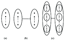
Figure 1: The diagrams for the single quantum state (a), product state (b), and ensemble-product state (c). The circle stands for the scope, and the points within stand for the orthogonal eigenstates (the total number is assumed to be $d$, thus, qu$d$it). The correlation between scopes or states is depicted as straight line (string).

QM often deals with the properties of many-body (instead of single or infinite) system. To characterize the quantum features, at present, there exist three widely studied methods: nonlocality bell87 , nonclassicality glauber , and entanglement horodecki . Traditionally, nonclassicality was introduced in the quantum phase-space in the context of Quantum Optics. The state of light, e.g., squeezed light, contains nonclassicality compared with the coherent light, which sets the boarder between quantum and classical states. We note that the continuous variable (CV) system in phase-space can be translated into the Fock space, from which the entanglement can be defined. Interestingly, after the seminal work of EPR epr and Bell bell87 , the nonlocality of entangled state was demonstrated with nonclassical light aspect , where the three methods are all involved. In this work, we do not intend to analyze the relations of them; instead, we focus on entanglement relating to superposition and the concept of scope. Part of our study on entanglement has been presented in Ref. wang . We will study the physical role of entanglement in various quantum states, and the degree of entanglement, also we compare with different entanglement measure in Appendix D.

Entanglement is widely studied in QIQC, and it is believed to be the key for information processing and computing. However, entanglement is not indispensable. In quantum cryptography, the BB$84$ does not rely on entanglement bb84 ; instead, particularly the B$92$ protocol shows that it is the nonorthogonality (also no-cloning) that ensures the security of the key b92 . The recently studied continuous variable (CV)-quantum key distribution (QKD) Grosshans and decoy-state QKD Lo , also do not rely on entanglement, which indeed are the improvement of the BB$84$ protocol. This indicates that the quantum nature of information acts even when there is no entanglement, i.e., the quantum information does not necessarily depends on entanglement. In quantum computing, the well-known QDC$1$ model is shown not directly rely on entanglement Knill ; instead, the quantum discord plays the central role Datta . In another line of research, there are attempts to build QKD on the foundation of nonlocality and nonlocal box, where entanglement does not play the central role popescu ; Barrett .

The examples above indicate that entanglement is not such quantity viewed from the information-theoretic framework (ITF), which is the theoretic paradigm or the world view correlating with the research of QIQC to re-consider quantum theory and its foundation from the information point, where information is believed as physical and fundamental Bub ; Wheeler1 ; Wheeler2 ; Landauer . On the contrary, especially from the concept of scope, entanglement is the direct generalization of superposition, not necessarily related to information (entropy), physically. The original CV-entangled state of EPR epr and (discrete variable) DV-entangled state of spin of Bohm Bohm do not relate to information. The analysis of Schrödinger just reveals that information can be effected by entanglement Schrodinger . Also, entanglement does not only play roles in QIQC. For instance, in quantum chemistry, entanglement plays roles in the formation of molecules and chemical reactions. Further, the so-called “quantum information” is quite misleading, as the Zeilinger’s principle Zeilinger99 states that there is no quantum information, there is only information processing with quantum sources. That is to say, information can be effected by the quantum features, including nonorthogonality (superposition), entanglement, also nonlocality and nonclassicality.

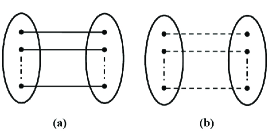
Figure 2: The diagrams for the entangled qudit (a), and decohered qudit (b). The straight lines (string) stand for the correlation, the dashed lines stand for decohered correlation.

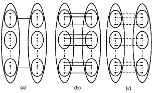
Figure 3: The diagrams for the separable state (a), ensemble-entangled qudit (b), and ensemble-decohered qudit (c).

IV.2 Quantum states

In this section, we will systematically study the quantum correlations of the bi-party system, the results for the multi-party system will be presented in other places. Also, without loss of generality, we assume here that the branches within the entangled scope are all realized, i.e. mathematically, the entangled state is the same with the entangled scope. Relating to the analysis in Sec. II.2, the entangled state can be realized both for single quantum system and the ensemble of quantum system. The quantum states we analyze include:

• product state; entangled qudit; decohered qudit;

• ensemble-product state; separable state; ensemble-entangled qudit; ensemble-decohered qudit.

For clarity of the physical picture, we develop a kind of diagram to represent the scope. As shown in Fig. 1(a), the circle stands for the scope, and the points within stand for the orthogonal eigenstates (with number $d$). The correlation between scopes or states is depicted as straight line (string), the dashed line stands for decohered string. The states we consider are shown in Fig. [1-3].

Product state. As well-known, product state contains no correlation. Here, we can describe three kinds of product states. Suppose the two sub-systems are $A$ and $B$, with orthogonal eigenstate $\{A_{i}\}$ and $\{B_{i}\}$, respectively.

(a). The state $|A_{i}\rangle\otimes|B_{i}\rangle$ is product state.

(b). The more complex product form is

$$\rho_{P}=\rho_{A}\otimes\rho_{B}=|\psi_{A}\rangle\langle\psi_{A}|\otimes|\psi_{B}\rangle\langle\psi_{B}|,$$ (21)

where $|\psi_{A}\rangle=\sum_{i}a_{i}|A_{i}\rangle$, $|\psi_{B}\rangle=\sum_{i}b_{i}|B_{i}\rangle$. We note that the states for $A$ and $B$ are not ensemble. This product state is shown in Fig. 1(b).

(c). The third kind is the ensemble-product state, shown in Fig. 1(c). The wave functions of the systems $A$ and $B$ can be written as

$$|\psi_{A}\rangle = \sum_{\xi}\gamma_{\xi}|\psi_{\xi}^{A}\rangle,$$

$$|\psi_{B}\rangle = \sum_{\xi}\gamma_{\xi}|\psi_{\xi}^{B}\rangle,$$ (22)

which is the coarse-grained decomposition, since there exist the sub- wave functions $|\psi_{\xi}^{A}\rangle=\sum_{i}a^{\xi}_{i}|A_{i}\rangle$, $|\psi_{\xi}^{B}\rangle=\sum_{i}b^{\xi}_{i}|B_{i}\rangle$, and generally $\langle\psi_{\xi}^{A(B)}|\psi_{\xi^{\prime}}^{A(B)}\rangle\neq 0$. With $p_{\xi}=|\gamma_{\xi}|^{2}$, the density matrix can be easily written as

$$\rho_{A} = \sum_{\xi}p_{\xi}|\psi_{\xi}^{A}\rangle\langle\psi_{\xi}^{A}|=\sum_{\xi}p_{\xi}\rho_{\xi}^{A},$$

$$\rho_{B} = \sum_{\xi}p_{\xi}|\psi_{\xi}^{B}\rangle\langle\psi_{\xi}^{B}|=\sum_{\xi}p_{\xi}\rho_{\xi}^{B}.$$ (23)

The ensemble-product state is

$$\rho_{eP}=\rho_{A}\otimes\rho_{B}=(\sum_{\xi}p_{\xi}\rho_{\xi}^{A})\otimes(\sum_{\xi}p_{\xi}\rho_{\xi}^{B}).$$ (24)

The state $\rho_{eP}$ contains quantum information, although there is no entanglement. There is coherence for the $\rho_{\xi}^{A}$ and $\rho_{\xi}^{B}$, that is, there can be decoherence process. The result of the decoherence is that the local state of $A$ and $B$ become $\rho_{\xi}^{A}=\sum_{i}(a^{\xi}_{i})^{2}|A_{i}\rangle\langle A_{i}|$, and $\rho_{\xi}^{B}=\sum_{i}(b^{\xi}_{i})^{2}|B_{i}\rangle\langle B_{i}|$. Yet, the global state $\rho_{ep}$ remains as product.

Entangled qudit. The general form of the entangled qudit is written as

$$|\Psi_{E}\rangle=\frac{\sum_{i}a_{i}b_{i}|A_{i}\rangle\otimes|B_{i}\rangle}{\sqrt{\sum_{i}a_{i}^{2}b_{i}^{2}}},$$ (25)

and the density matrix is expressed as

$$\rho_{E}=|\Psi_{E}\rangle\langle\Psi_{E}|=\frac{\sum_{i,j}\eta_{i}\eta_{j}|A_{i}\rangle\langle A_{j}|\otimes|B_{i}\rangle\langle B_{j}|}{\sum_{i}\eta_{i}^{2}},$$ (26)

with $\eta_{i}=a_{i}b_{i}$.

The state $\rho_{E}$, shown in Fig. 2(a), can be viewed as a part of the product state $\rho_{P}$ in case (b) above, by selecting out the branches according to the permutation symmetry. The coherence of the state $\rho_{E}$ is represented by the non-diagonal elements. When decoherence occurs by some disturbance, the state $\rho_{E}$ becomes diagonal, which is said to be classical. The decohered (classical) qudit is

$$\rho_{D} = \sum_{i}\eta^{2}_{i}|A_{i}\rangle\langle A_{i}|\otimes|B_{i}\rangle\langle B_{i}|/\sum_{i}\eta^{2}_{i}$$ (27)

$$= \sum_{i}a_{i}^{2}b_{i}^{2}\rho_{i}^{A}\otimes\rho^{B}_{i}/\sum_{i}a^{2}_{i}b^{2}_{i}.$$

Let $\rho_{A}=\sum_{i}a_{i}^{2}\rho_{i}^{A}$, $\rho_{B}=\sum_{i}b_{i}^{2}\rho_{i}^{B}$, and introduce the parameter $p_{i}=\eta^{2}_{i}/\sum_{i}\eta^{2}_{i}$, then

$$\rho_{D}=\sum_{i}p_{i}\rho_{i}^{A}\otimes\rho_{i}^{B},$$ (28)

which is separable. That is, for the single decohered qudit, it is classical as well as separable. This state is shown in Fig. 2(b).

Separable state. The well-known separable state Werner89 in Fig. 3(a) is defined as

$$\rho_{S}=\sum_{\xi}p_{\xi}\rho_{\xi}^{A}\otimes\rho_{\xi}^{B},$$ (29)

with the normalization relation $\sum_{\xi}p_{\xi}=1$.

We show that the separable state $\rho_{S}$ is the analogy of entangled state $\rho_{E}$, except that the former one employs the coarse-grained decomposition, while the latter one employs the fine-grained decomposition, i.e., the eigenstates are orthogonal. The decomposition is the same with those in equations (22) and (23). Then equation (29) can be written as

$$\rho_{S}=\sum_{\xi}p_{\xi}(\sum_{k,l}a_{k}^{\xi}a_{l}^{\xi*}|A_{k}\rangle\langle A_{l}|)\otimes(\sum_{m,n}b_{m}^{\xi}b_{n}^{\xi*}|B_{m}\rangle\langle B_{n}|),$$ (30)

which is the analogy of equation (26).

The ensemble (sets) $\{|\psi_{\xi}^{A}\rangle\}$ and $\{|\psi_{\xi}^{B}\rangle\}$ are not classical, while the ensemble $\{|A_{i}\rangle\}$ and $\{|B_{i}\rangle\}$ are classical. This reveals that there exists quantum information in the separable state. Then, when the separable state goes to the classical state? Consider the case when only one eigenstate each is acted out, that is $d=1$, and also let $\langle\psi_{\xi}^{A(B)}|\psi_{\xi^{\prime}}^{A(B)}\rangle=0$. Then the density matrix $\rho_{S}$ in equation (30) becomes the same with the classical state $\rho_{D}$ in equation (27). We can label this as the “classical reduction procedure”.

Let us give a simple example of the $2\otimes 2$ system. It is reasonable to set $|\psi_{1}^{A(B)}\rangle=\left(\begin{array}[]{c}1\\ 0\end{array}\right)$, and $|\psi_{2}^{A(B)}\rangle=\left(\begin{array}[]{c}0\\ 1\end{array}\right)$, then the separable state is

$$\rho_{S}=\left(\begin{array}[]{cccc}p_{1}&0&0&0\\ 0&0&0&0\\ 0&0&0&0\\ 0&0&0&p_{2}\end{array}\right),$$ (31)

which is also classical.

Generally, when $d\neq 1$, the separable form of the density matrix does not rely on the local coherence within $\rho_{\xi}^{A}$ and $\rho_{\xi}^{B}$, which just indicates that there can be quantum information in the separable state.

Ensemble-entangled qudit. The ensemble of entangled state is often studied in QIQC, such as the ensemble of Bell’s state. For single entangled qudit, it can be written in the Schmidt basis as

$$|\psi_{\xi}\rangle=\sum_{i}\lambda^{\xi}_{i}|A_{i}\rangle|B_{i}\rangle,$$ (32)

with $\sum_{i}(\lambda^{\xi}_{i})^{2}=1$. The density matrix of this ensemble can be expressed as

$$\rho_{eE} = \sum_{\xi}p_{\xi}|\psi_{\xi}\rangle\langle\psi_{\xi}|$$

$$= \sum_{\xi}p_{\xi}\sum_{i}\lambda^{\xi}_{i}|A_{i}\rangle|B_{i}\rangle\sum_{j}\lambda^{\xi*}_{j}\langle A_{j}|\langle B_{j}|$$

$$= \sum_{\xi}p_{\xi}\sum_{i,j}\lambda^{\xi}_{i}\lambda^{\xi*}_{j}|A_{i}\rangle\langle A_{j}|\otimes|B_{i}\rangle\langle B_{j}|$$

$$\neq \rho_{S}.$$

The ensemble-entangled qudit is shown in Fig. 3(b). It is easy to see that when applies the classical reduction procedure, $d=1$, and $\langle\psi_{\xi}^{A(B)}|\psi_{\xi^{\prime}}^{A(B)}\rangle=0$, the state $\rho_{eE}$ reduces to classical and also separable.

When decoherence occurs, each entangled qudit becomes classically correlated, and the ensemble-decohered qudit is

$$\rho_{eD}=\sum_{\xi}p_{\xi}\sum_{i}(\lambda^{\xi}_{i})^{2}|A_{i}\rangle\langle A_{i}|\otimes|B_{i}\rangle\langle B_{i}|,$$ (34)

which is classical but not separable, shown in Fig. 3(c).

Further, to make the distinctions of the quantum states clear, we can classify four kinds of correlations: entanglement, decohered classicality, nonorthogonality, and coarse-grained classicality. The quantum characters in the states we studied are different. In the single entangled qudit, the entanglement is the global shared coherence, there is also the classical correlation. For the decohered qudit, the shared coherence disappears, thus there is only classicality. The ensemble-entangled qudit, which relies on the coarse-grained decomposition, contains another kind of shared coherence due to nonorthogonal local states, namely, $\langle\psi_{\xi}^{A(B)}|\psi_{\xi^{\prime}}^{A(B)}\rangle\neq 0$, we name it as nonorthogonality. Correspondingly, there exists another kind of classicality, via the parameter $p_{\xi}$, instead of the correlations of the eigenstates between $A$ and $B$. We name this kind of correlation as coarse-grained classicality, and the former one as decohered classicality. From this analysis, we can briefly present the main characters of quantum state in TABLE I.

Table 1: The main characters of the quantum states. The four kinds of correlations are shown on the left, the six kinds of quantum states are shown on the top. $\surd$ ($\times$) means the corresponding state has (does not have) the corresponding correlation.

	qudit	decohered qudit	ensemble qudit	ensemble-decohered qudit	separable	ensemble-product
entanglement	$\surd$	$\times$	$\surd$	$\times$	$\times$	$\times$
decohered classicality	$\surd$	$\surd$	$\surd$	$\surd$	$\times$	$\times$
nonorthogonality	$\times$	$\times$	$\surd$	$\surd$	$\surd$	$\surd$
coarse-grained classicality	$\times$	$\times$	$\surd$	$\surd$	$\surd$	$\times$

IV.3 Degree of superposition and entanglement

In this section, we study superposition and entanglement quantitatively. Before our analysis, we note that the superposition and entanglement are both due to the existence of coherence, local and global (shared), respectively. Entanglement is not the quantum information; instead, the classical information (correlation) can be effected by the entanglement (shared coherence), thus, the so-called “quantum information”. We can say that entanglement and quantum information (entropy) are the two related kinds of characters of the entangled state. Below, we present the definitions of the degree of superposition, entanglement, and nonorthogonality, which all relate to the quantum coherence.

Definition 1

Degree of superposition $\varepsilon$.

For a superposed state vector $|\Psi\rangle=\sum_{i}^{n}a_{i}|\psi_{i}\rangle$, where $\sum_{i}^{n}|a_{i}|^{2}=1$, $\langle\psi_{i}|\psi_{j}\rangle=0$, the degree of superposition

$$\varepsilon\equiv\sum_{i<j}^{n}|a_{i}||a_{j}|.$$ (35)

Notice that, by introducing the $l_{2}$-norm as $||a||_{l_{2}}$$=\sum_{i}^{n}|a_{i}|^{2}$, then the $l_{1}$-norm is $||a||_{l_{1}}$$=\sum_{i}^{n}|a_{i}|$, thus, $\varepsilon=\frac{1}{2}{(||a||_{l_{1}}^{2}-||a||_{l_{2}})}$. This indicates that the $l_{1}$-norm has physical meaning, i.e., describing the degree of superposition.

Let us show some examples. When $n=1$, $\varepsilon=0$. $n=2$, $|\Psi\rangle=a_{1}|\psi_{1}\rangle+a_{2}|\psi_{2}\rangle$, $\varepsilon=|a_{1}a_{2}|$, and Max($\varepsilon$)$=1/2$ when $|a_{1}|=|a_{2}|=1/\sqrt{2}$. $n=3$, $|\Psi\rangle=a_{1}|\psi_{1}\rangle+a_{2}|\psi_{2}\rangle+a_{3}|\psi_{3}\rangle$, $\varepsilon=|a_{1}a_{2}|+|a_{2}a_{3}|+|a_{1}a_{3}|$, and Max($\varepsilon$)$=1$ when $|a_{1}|=|a_{2}|=|a_{3}|=1/\sqrt{3}$. Then generally, for $n=4,5,...$, Max($\varepsilon$)$=3/2,2,...$ etc. That is, for $n$, the maximal degree of superposition $\varepsilon$ is $\frac{n-1}{2}$, and the minimum approaches to zero. If there are more eigenstates in a superposed state, then the degree of superposition it can get is bigger. It means, physically, that although a state vector in the Hilbert space has to be normalized, the degree of superposition is not a relative quantity, it characterizes the amount of coherence.

Definition 2

Degree of entanglement $\mathcal{E}$.

For a general entangled state with $m$ subsystems $n\otimes n\otimes...\otimes n$ with each $n$-dimensional: $|\Psi\rangle=\sum_{i}^{n}c_{i}|\psi_{1i}\psi_{2i}...\psi_{mi}\rangle$, the degree of entanglement

$$\mathcal{E}\equiv\sum_{i<j}^{n}|c_{i}||c_{j}|.$$ (36)

The same with the degree of superposition, we can get $\mathcal{E}=\frac{1}{2}{(||c||_{l_{1}}^{2}-||c||_{l_{2}})}$.

Our definition $2$ is similar with negativity (see Appendix D), thus, we do not present the proof of the entanglement monotone horodecki , which states that the entanglement cannot increase under the local quantum operation and classical communication (LOCC). According to our understanding based on scope and coherence, the LOCC constraint is the property of quantum information (entropy) instead of entanglement (globally shared coherence). Yet, it is easy to check that entanglement obviously satisfies the LOCC constraint since the quantum coherence cannot be created via classical way. The definition $2$ defines entanglement in a positive way. As a result, the LOCC constraint is not sufficient to define entanglement, and not all non-separable states are entangled (Sec. IV.2).

Next we study some basic applications. We assume the coefficients are all positive, without loss of generality.

For $2\otimes 2$ system, if

$$|\Psi_{A}\rangle = a_{1}|\psi_{1}\rangle+a_{2}|\psi_{2}\rangle,\varepsilon_{A}=a_{1}a_{2},$$ (37)

$$|\Psi_{B}\rangle = b_{1}|\psi_{1}\rangle+b_{2}|\psi_{2}\rangle,\varepsilon_{B}=b_{1}b_{2}.$$

Label $|\psi_{1}\rangle=|1\rangle$, $|\psi_{2}\rangle=|2\rangle$. There are two kinds of entangled state according to the nature of the branches (strings). If $|1(2)\rangle$ of $A$ correlates with $|1(2)\rangle$ of $B$, it is named as “direct” ($|\Psi_{d}\rangle$); if $|1(2)\rangle$ correlates with $|2(1)\rangle$, it is named as “cross” ($|\Psi_{c}\rangle$):

$$|\Psi_{d}\rangle = \frac{a_{1}b_{1}|11\rangle+a_{2}b_{2}|22\rangle}{\sqrt{a_{1}^{2}b_{1}^{2}+a_{2}^{2}b_{2}^{2}}},$$ (38)

$$|\Psi_{c}\rangle = \frac{a_{1}b_{2}|12\rangle+a_{2}b_{1}|21\rangle}{\sqrt{a_{1}^{2}b_{2}^{2}+a_{2}^{2}b_{1}^{2}}},$$

and the degree of entanglement

$$\mathcal{E}_{d} = \frac{a_{1}a_{2}b_{1}b_{2}}{a_{1}^{2}b_{1}^{2}+a_{2}^{2}b_{2}^{2}},$$ (39)

$$\mathcal{E}_{c} = \frac{a_{1}a_{2}b_{1}b_{2}}{a_{1}^{2}b_{2}^{2}+a_{2}^{2}b_{1}^{2}},$$

generally, $\mathcal{E}_{d}\neq\mathcal{E}_{c}$.

After some algebra, we can get

$$\frac{\varepsilon_{A}\varepsilon_{B}}{\mathcal{E}_{d}}+\frac{\varepsilon_{A}\varepsilon_{B}}{\mathcal{E}_{c}}=1.$$ (40)

Introduce the reduced degree of entanglement

$$\mathcal{E}^{\dagger}=\frac{\mathcal{E}_{d}\mathcal{E}_{c}}{\mathcal{E}_{d}+\mathcal{E}_{c}},$$ (41)

then we can get the fundamental relation

$$\mathcal{E}^{\dagger}=\varepsilon_{A}\varepsilon_{B}.$$ (42)

When $a_{1}=a_{2}=b_{1}=b_{2}=\sqrt{2}/2$, $\varepsilon_{A}=\varepsilon_{B}=1/2$, $|\Psi_{d}\rangle=\frac{\sqrt{2}}{2}{(|11\rangle+|22\rangle)}$, $|\Psi_{c}\rangle=\frac{\sqrt{2}}{2}{(|12\rangle+|21\rangle)}$, $\mathcal{E}_{d}=\mathcal{E}_{c}=1/2$, and $\mathcal{E}^{\dagger}=1/4$. This is the maximal condition for the qubit.

In addition, for the reduced degree of entanglement of the qubit system, we will further study the physical properties by comparing to the classical two-body problem in Appendix C.

For $2\otimes 2\otimes 2$ system, if

$$|\Psi_{A}\rangle = a_{1}|\psi_{1}\rangle+a_{2}|\psi_{2}\rangle,\varepsilon_{A}=a_{1}a_{2},$$ (43)

$$|\Psi_{B}\rangle = b_{1}|\psi_{1}\rangle+b_{2}|\psi_{2}\rangle,\varepsilon_{B}=b_{1}b_{2},$$

$$|\Psi_{C}\rangle = c_{1}|\psi_{1}\rangle+c_{2}|\psi_{2}\rangle,\varepsilon_{C}=c_{1}c_{2}.$$

There are four kinds of entangled state, which belongs to the Greenberger-Horne-Zeilinger (GHZ) state ghz :

$$|\Psi_{GHZ}^{1}\rangle = \frac{a_{1}b_{1}c_{1}|111\rangle+a_{2}b_{2}c_{2}|222\rangle}{\sqrt{a_{1}^{2}b_{1}^{2}c_{1}^{2}+a_{2}^{2}b_{2}^{2}c_{2}^{2}}},$$ (44)

$$|\Psi_{GHZ}^{2}\rangle = \frac{a_{1}b_{1}c_{2}|112\rangle+a_{2}b_{2}c_{1}|221\rangle}{\sqrt{a_{1}^{2}b_{1}^{2}c_{2}^{2}+a_{2}^{2}b_{2}^{2}c_{1}^{2}}},$$

$$|\Psi_{GHZ}^{3}\rangle = \frac{a_{2}b_{1}c_{1}|211\rangle+a_{1}b_{2}c_{2}|122\rangle}{\sqrt{a_{2}^{2}b_{1}^{2}c_{1}^{2}+a_{1}^{2}b_{2}^{2}c_{2}^{2}}},$$

$$|\Psi_{GHZ}^{4}\rangle = \frac{a_{1}b_{2}c_{1}|121\rangle+a_{2}b_{1}c_{2}|212\rangle}{\sqrt{a_{1}^{2}b_{2}^{2}c_{1}^{2}+a_{2}^{2}b_{1}^{2}c_{2}^{2}}},$$

and it is easy to write the four degree of entanglement (we do not present here), after some algebra, we get

$$\frac{\varepsilon_{A}\varepsilon_{B}\varepsilon_{C}}{\mathcal{E}_{1}}+\frac{\varepsilon_{A}\varepsilon_{B}\varepsilon_{C}}{\mathcal{E}_{2}}+\frac{\varepsilon_{A}\varepsilon_{B}\varepsilon_{C}}{\mathcal{E}_{3}}+\frac{\varepsilon_{A}\varepsilon_{B}\varepsilon_{C}}{\mathcal{E}_{4}}=1.$$ (45)

Also, introduce the reduced degree of entanglement

$$\mathcal{E}^{\dagger}=\frac{\mathcal{E}_{1}\mathcal{E}_{2}\mathcal{E}_{3}\mathcal{E}_{4}}{\mathcal{E}_{1}\mathcal{E}_{2}\mathcal{E}_{3}+\mathcal{E}_{1}\mathcal{E}_{2}\mathcal{E}_{4}+\mathcal{E}_{1}\mathcal{E}_{3}\mathcal{E}_{4}+\mathcal{E}_{2}\mathcal{E}_{3}\mathcal{E}_{4}},$$ (46)

then

$$\mathcal{E}^{\dagger}=\varepsilon_{A}\varepsilon_{B}\varepsilon_{C}.$$ (47)

For the maximal condition, when all the coefficients equal to $\sqrt{3}/3$, $\varepsilon_{A}=\varepsilon_{B}=\varepsilon_{C}=1/2$, $\mathcal{E}_{1}=\mathcal{E}_{2}=\mathcal{E}_{3}=\mathcal{E}_{4}=1/2$, and $\mathcal{E}^{\dagger}=1/8$.

Generally, for $2~{}\otimes^{n}$ system, the maximal reduced entanglement is $\mathcal{E}^{\dagger}=1/2^{n}$. This means when we add the numbers of systems to be entangled, the reduced entanglement becomes smaller and smaller, that is, the entanglement of the whole system becomes more fragile, when one subsystem is disturbed, the total entanglement vanishes.

For $3\otimes 3$ system, if

$$|\Psi_{A}\rangle = a_{1}|\psi_{1}\rangle+a_{2}|\psi_{2}\rangle+a_{3}|\psi_{3}\rangle,$$ (48)

$$|\Psi_{B}\rangle = b_{1}|\psi_{1}\rangle+b_{2}|\psi_{2}\rangle+b_{3}|\psi_{3}\rangle,$$

and the degree of superposition

$$\varepsilon_{A} = a_{1}a_{2}+a_{2}a_{3}+a_{1}a_{3},$$ (49)

$$\varepsilon_{B} = b_{1}b_{2}+b_{2}b_{3}+b_{1}b_{3}.$$

There are six kinds of entangled state according to the symmetry between the branches within the entangled state. Here we only give two examples, the other four are easy to be drawn:

$$|\Psi_{1}\rangle = \frac{a_{1}b_{1}|11\rangle+a_{2}b_{2}|22\rangle+a_{3}b_{3}|33\rangle}{\sqrt{a_{1}^{2}b_{1}^{2}+a_{2}^{2}b_{2}^{2}+a_{3}^{2}b_{3}^{2}}},$$ (50)

$$|\Psi_{2}\rangle = \frac{a_{1}b_{2}|12\rangle+a_{2}b_{1}|21\rangle+a_{3}b_{3}|33\rangle}{\sqrt{a_{1}^{2}b_{2}^{2}+a_{2}^{2}b_{1}^{2}+a_{3}^{2}b_{3}^{2}}}.$$

The entanglements of these six states have the form $\mathcal{E}_{i}=\alpha_{i}/\beta_{i}$. After some algebra, we can get

$$\sum_{i}^{6}\frac{\alpha_{i}}{\mathcal{E}_{i}} = \sum_{i}^{6}\beta_{i}=2,$$ (51)

$$\sum_{i}^{6}\alpha_{i} = 2\varepsilon_{A}\varepsilon_{B}.$$

For the maximal condition, when $\alpha_{i}=1/3$, $\beta_{i}=1/3$, $\varepsilon_{A}=\varepsilon_{B}=1$, $\mathcal{E}_{i}=1$. For this bi-qutrit entangled state, there is no definite form of reduced entanglement.

For $4\otimes 4$ system, there exist totally twenty-four different states, each has four branches. The entanglement also can be written as $\mathcal{E}_{i}=\alpha_{i}/\beta_{i},i=1,2,...24$. We get the following equations

$$\sum_{i}^{24}\frac{\alpha_{i}}{\mathcal{E}_{i}} = \sum_{i}^{24}\beta_{i}=6,$$ (52)

$$\sum_{i}^{24}\alpha_{i} = 4\varepsilon_{A}\varepsilon_{B}.$$

For the maximal condition, when $\alpha_{i}=3/8$, $\beta_{i}=1/4$, $\varepsilon_{A}=\varepsilon_{B}=3/2$, $\mathcal{E}_{i}=3/2$.

Generally, for $n\otimes n$ system, there are $N=n!$ different entangled states, set $\mathcal{E}_{i}=\alpha_{i}/\beta_{i}$, we can get the general equations as

$$\sum_{i}^{N}\frac{\alpha_{i}}{\mathcal{E}_{i}} = \sum_{i}^{N}\beta_{i}=(n-1)!,$$ (53)

$$\sum_{i}^{N}\alpha_{i} = 2(n-2)!\varepsilon_{A}\varepsilon_{B}.$$

For the maximal condition, when $\alpha_{i}=(n-1)/2n$, $\beta_{i}=1/n$, $\varepsilon_{A}=\varepsilon_{B}=(n-1)/2$, $\mathcal{E}_{i}=(n-1)/2$. That is, for the two-party systems, when the number of states entangled together increases, the Max($\mathcal{E}$) also increases, like the superposition $\varepsilon$. This is reasonable since when more states are entangled together, the amount of entanglement should increase, and the state becomes more robust.

For the higher dimensional systems, the math is a little complex, and the physical picture is not so clear. We do not analyze them here. Next, we turn to the quantization of the four kinds of correlations we defined in the last subsection.

For the entangled qudit, the entanglement is the shared coherence, so the degree of entanglement $\mathcal{E}$ can be easily calculated, according to the definition 36 above. Also, as we have discussed, we can employ different forms of entropy to characterize the quantum information. At present, the well-known quantities include von Neumann entropy, relative entropy, quantum discord, squashed entanglement, entanglement of formation, cost, and distillation, etc Peres ; Vidal02 ; bbps ; Hill ; Bennett ; Vedral ; Vidal99 ; Steiner ; Ollivier ; Luo ; Christandl ; Brandao ; Gittsovich . We will study some of them in Appendix D.

For the decohered qudit, there is pure classical correlation without shared quantum coherence. Also, there exist the complete projective measurements, under which the classical density matrix remains Ollivier ; Luo . The information is characterized by the von Neumann entropy.

For the four kinds of ensemble state, see TABLE I, there exists nonorthogonality. This kind of coherence is not globally shared by the two parties $A$ and $B$, yet, it is shared by the local states $|\psi_{\xi}^{A}\rangle$ of $A$, and the local states $|\psi_{\xi}^{B}\rangle$ of $B$. The degree of nonorthogonality can be defined as

$$\mathcal{\bar{O}}=\sum_{\mu=A,B}\sum_{\xi\neq\xi^{\prime}}|\langle\psi_{\xi}^{\mu}|\psi_{\xi^{\prime}}^{\mu}\rangle|.$$ (54)

In the sum, each element is smaller than one, yet, the sum can be arbitrarily big even infinity. This is reasonable since the quantity of coherence increases with the amount of the ensemble. Particularly, we note that the separable state contains the quantum nonorthogonality thus quantum information, although there is no entanglement.

The coarse-grained classicality results from the classical parameter $p_{\xi}$, so the classical information can be easily calculated via the von Neumann entropy $S=-\sum_{\xi}p_{\xi}\log p_{\xi}$.

Last, we make some comments on the mixed state, which, in deed, is a rather broad and rough method. The mixed state with purity smaller than unity is a “fragment” of a global pure state with an unknown part lost, thus, it is not easy to decide the exact structure of the mixed state. At present, there exist lots of ways to detect the entanglement, and different methods can be unified with the method of entanglement witness in a way Brandao . Yet, even we can find the entanglement, we cannot decide the structure of the mixed state. That is to say, to find how the mixed state is formed is more valuable and practical. The six kinds of states studied above can serve as some standard or assistant to detect the quantum correlations. When a mixed state $\rho$ can be written as similar to any standard state, labeled as $\sigma$, that is, if $\rho=\lambda\sigma+(1-\lambda)\rho^{\prime}$, then the quantum correlation (entanglement, nonorthogonality, etc) of $\rho$ can be defined as that of $\sigma$ times $\lambda$. $\rho^{\prime}$ can be viewed as the disturbance or perturbation to $\sigma$. This method is similar with the relative entropy method Vidal99 and the Lewenstein-Sanpera (LS) decomposition Sanpera .

To sum up, in this section, we quantify the degree of superposition and entanglement, and also nonorthogonality. Physically, entanglement is directly based on superposition, and nonorthogonality is also the result of superposition. The four kinds of correlations can be easily calculated.

V CONCLUSION

The weirdness of QM is a result of the nature of quantum coherence, the abstractness of quantum description, and the confusions on quantum logic and philosophy. The concept of scope, which is exotic for CM, Relativity, statistical mechanics, also classical wave mechanics, just represents the quantum origin. It describes the possible (potential) action region and the systematic and coherent structure of movement of a certain object. Superposition and entanglement are the natural results of scope with definite physical meaning. Also, we discussed the properties of four kinds of quantum correlations and the six kinds of quantum states, and we show that entanglement is related yet different with entropy. Further, the concept of scope brings new methods to the standard QM. One is that the scope itself has certain geometric features, just similar to the matter itself. This may indicate that the structure of the motion of the matter is more crucial than the structure of the matter itself. The other is that, rather than the information-theoretic framework, there exists a new kind of space, i.e., tangnet, on which the quantum structure with entanglement exists wang . As a result, the concept of scope lays the new starting point to the foundation of QM. In the future, further efforts on, e.g., the geometrical properties of tangnet, the comparison of scope with other interpretations, also the relation between nonlocality and entanglement, are needed.

In addition, the physical roles of entanglement in QIQC are also widely concerned, we hope our approach can bring new ideas on some tough problems, such as the bound entanglement bound , the analogy of entanglement to energy or entropy, etc.

Appendix A Wave function of Ensemble system and Decoherence

In Hilbert space, one state vector can be decomposed via orthogonal basis also non-orthogonal basis. Physically, the two decompositions can be endowed with different physical contents: for single system, there only exists orthogonal physical basis; while for ensemble, there can be non-orthogonal basis. For example, the spin state in one quantum dot can be up or down, or to the left or right in the diagonal basis; for a collection of spins in quantum dots, the superposed states of spins form the non-orthogonal basis. Mathematically, based on the measurement theory, especially the positive operator-valued measure (POVM) Nielsen , we can see the WFES has the corresponding properties as the wave function of pure state.

For the pure state $|\phi\rangle=\sum_{i}c_{i}|i\rangle$, it satisfies: (1) Normalization: $\sum_{i}|c_{i}|^{2}=1$; (2) Completeness relation: $\sum_{i}|i\rangle\langle i|=1$; (3) Projective measurement: there exist a set of projective operators $\{\hat{P}_{i}=|i\rangle\langle i|\}$ satisfying $\hat{P}_{i}|\phi\rangle=c_{i}|i\rangle$, the expectation value $\langle\hat{P}_{i}\rangle=|c_{i}|^{2}$; note that when the non-projective POVM operator acts on the pure state, it cannot distinguish its basis; (4) Probabilistic interpretation: $|c_{i}|^{2}$ means the probability to find state $|i\rangle$ with projector $\hat{P}_{i}$; (5) Observable: the expectation value of observable $\hat{A}$ is $\langle\hat{A}\rangle=\sum_{i}a_{i}|c_{i}|^{2}$, with $\hat{A}|i\rangle=a_{i}|i\rangle$; (6) Evolution: $|\phi\rangle$ also the basis $|i\rangle$ satisfy Schrödinger equation; (7) Decoherence: the non-diagonal elements in $|\phi\rangle\langle\phi|$ disappear, leading to state $\rho=\sum_{i}|c_{i}|^{2}|i\rangle\langle i|$, each part $|c_{i}|^{2}|i\rangle\langle i|$ forms the classical trajectory; (8) Quantum reference frame Rudolph : to determine the preferred basis $\{|i\rangle\}$, the reference frame and certain interaction are needed to form the entangled state, i.e., the coherence within $|\phi\rangle$ delocalizes to form entanglement; thus, by ignoring the reference frame, the state $|\phi\rangle$ decohered.

For the WFES, the state in Eq. (6), the properties are similar while more complicated. We firstly note that if $k=1$, it reduces to the pure state case; if the states $\{|\psi_{k}\rangle\}$ are orthogonal with each other, it goes to the totally classical (decohered) state. Instinctively, there exists one pure density matrix, labeled as $\varrho\equiv|\Psi\rangle\langle\Psi|$, which is

$$\varrho=\sum_{k,k^{\prime}}\gamma_{k}\gamma_{k^{\prime}}|\psi_{k}\rangle\langle\psi_{k^{\prime}}|.$$ (55)

To form the density matrix $\rho$, the non-diagonal elements disappear, with coefficients $\gamma_{k}\gamma_{k^{\prime}\neq k}$, which is actually a kind of decoherence. The state $\varrho$ indicates that before the formation of the ensemble, there exists one decoherence process. Physically, the state $|\Psi\rangle$ stands for the “field” of the ensemble, and the ensemble emerges from the field after the decoherence process, i.e., the creation of particles Calzetta . Note that here we do not study this issue with quantum field theory. We name this kind of coherence as sub-coherence, or coarse-grained coherence, and the decoherence as sub-decoherence. To arrive at the classical state, the standard decoherence is then needed. If we only account coherence by ignoring sub-coherence, we can view $|\Psi\rangle$ as the WFES, from which, the density matrix $\rho$ for the ensemble emerges. Further, the sub-decoherence can be introduced by one quantum reference frame $\sigma\equiv\sum_{k,k^{\prime}}\gamma_{k}\gamma_{k^{\prime}}|\phi_{k}\rangle\langle\phi_{k^{\prime}}|$, which with $\varrho$ forms

$$\varpi=\sum_{k}|\gamma_{k}|^{2}|\psi_{k}\rangle\langle\psi_{k}|\otimes|\phi_{k}\rangle\langle\phi_{k}|,$$ (56)

which is exactly the separable state Werner89 . Note that for pure state, the system and its reference frame form the entangled state.

Correspondingly, the basic properties of WFES are: (1) Normalization: $\sum_{k}|\gamma_{k}|^{2}=1$; (2) Completeness relation: $\sum_{k}|\psi_{k}\rangle\langle\psi_{k}|=1$; (3) Measurement: there exist a set of POVM operators $\{\hat{E}_{k}=|\psi_{k}\rangle\langle\psi_{k}|\}$ satisfying $\hat{E}_{k}|\Psi\rangle=\gamma_{k}|\psi_{k}\rangle$, the expectation value $\langle\hat{E}_{k}\rangle=|\gamma_{k}|^{2}$; note that the measurement does not act on the fine-grained orthogonal basis directly; (4) Probabilistic interpretation: $|\gamma_{k}|^{2}$ means the probability to find state $|\psi_{k}\rangle$ with operator $\hat{E}_{k}$; (5) Observable: the expectation value of observable $\hat{A}$ is $\langle\hat{A}\rangle=\sum_{k}\alpha_{k}|\gamma_{k}|^{2}$, with $\hat{A}|\psi_{k}\rangle=\alpha_{k}|\psi_{k}\rangle$; (6) Evolution: states $|\Psi\rangle$ and $|\psi_{k}\rangle$ both satisfy Schrödinger equation, with which the Liouville equation for $\rho$ is equivalent; (7) Sub-decoherence: the non-diagonal elements in $|\Psi\rangle\langle\Psi|$ disappear, leading to quantum ensemble $\rho$; Decoherence: the party $|\psi_{k}\rangle$ each can further decohere, leading to classical state and classical trajectory, respectively; (8) Quantum reference frame: to determine the preferred basis $\{|\psi_{k}\rangle\}$, the reference frame $\sigma$ and certain interaction are needed to form the separable state, i.e., the sub-coherence within $|\Psi\rangle$ delocalizes to form separability; thus, by ignoring the reference frame, the state sub-decoheres; Further, if there exists the entanglement-type reference frame, the state eventually decoheres to classical trajectory.

Last, to illustrate the difference between coherence and sub-coherence, we give one simple example: suppose there are only two parties, $a$ and $b$, in the ensemble, and each party with only two orthogonal basis $|1\rangle$ and $|2\rangle$, and $|\psi_{a}\rangle=c_{1}^{a}|1\rangle+c_{2}^{a}|2\rangle$, $|\psi_{b}\rangle=c_{1}^{b}|1\rangle+c_{2}^{b}|2\rangle$. Note that even if party $b$ is not in the basis $|1,2\rangle$, there can be rotation which can rotate it to this basis, with effects absorbed in the coefficients. Thus, the density matrix of WFES is written as

$$\varrho=\left(\begin{array}[]{cc}|\gamma_{a}|^{2}|c_{1}^{a}|^{2}+|\gamma_{b}|^{2}|c_{1}^{b}|^{2}+\gamma_{a}\gamma_{b}^{*}c_{1}^{a}c_{1}^{b*}+\gamma_{b}\gamma_{a}^{*}c_{1}^{b}c_{1}^{a*}&|\gamma_{a}|^{2}c_{1}^{a}c_{2}^{a*}+|\gamma_{b}|^{2}c_{1}^{b}c_{2}^{b*}+\gamma_{a}\gamma_{b}^{*}c_{1}^{a}c_{2}^{b*}+\gamma_{b}\gamma_{a}^{*}c_{1}^{b}c_{2}^{a*}\\ |\gamma_{a}|^{2}c_{2}^{a}c_{1}^{a*}+|\gamma_{b}|^{2}c_{2}^{b}c_{1}^{b*}+\gamma_{a}\gamma_{b}^{*}c_{2}^{a}c_{1}^{b*}+\gamma_{b}\gamma_{a}^{*}c_{2}^{b}c_{1}^{a*}&|\gamma_{a}|^{2}|c_{2}^{a}|^{2}+|\gamma_{b}|^{2}|c_{2}^{b}|^{2}+\gamma_{a}\gamma_{b}^{*}c_{2}^{a}c_{2}^{b*}+\gamma_{b}\gamma_{a}^{*}c_{2}^{b}c_{2}^{a*}\end{array}\right).$$ (57)

The sub-coherence is represented as the coefficients $\gamma_{a}\gamma_{b}^{*}$ and its conjugate, when they disappear, the state $\varrho$ sub-decoheres to the quantum ensemble $\rho$. The coherence is represented as the coefficients $c_{1}^{a}c_{2}^{a*}$, $c_{1}^{a}c_{2}^{a*}$ and their conjugate, when they disappear, the state decoheres to the classical state, labeled as $\epsilon$, with diagonal elements $\epsilon_{11}=|\gamma_{a}|^{2}|c_{1}^{a}|^{2}+|\gamma_{b}|^{2}|c_{1}^{b}|^{2}$, $\epsilon_{22}=|\gamma_{a}|^{2}|c_{2}^{a}|^{2}+|\gamma_{b}|^{2}|c_{2}^{b}|^{2}$, and $\epsilon_{11}+\epsilon_{22}=1$.

Appendix B Scope and other methods

Scope and QFT. In QFT, the wave function is further viewed as the operator, which is the well-known “second quantization”. The total number of particles is not conserved as there always exist the fluctuations of field and creation/annihilatin of particles. Particle itself is viewed as the excited state of field, and field is viewed as a kind of matter, whose motion exists within itself. Thus, the second quantization of wave function, i.e., scope, means to view the structure of the motion as the equivalence of the structure of matter, also to view the motion of the matter as the same with the matter itself, which is reasonable for field. This is also consistent with the mass-energy relation $E=mc^{2}$ from Relativity. However, for particles, atoms etc in QM, the object itself is different with its motion, thus, it is not proper to view scope as a kind of matter; instead, scope should be viewed as a kind of description of the logical structure of the motion of the object.

In history, another physical picture similar with QFT is mainly developed by de Broglie, namely, the “pilot wave” approach debroglie , in which the particle with definite local form sits at a certain place in the real pilot wave, and the particle can be viewed as the high-energy concentrate singularity of the wave. The pilot-wave describes the collective motion of two objects: particle and wave, which indeed goes to the method of QFT. This relates to the “wave-particle duality” that the particle can perform both classical particle property and wave property, but not both of them at the same time Bohm . Also, the concept of “matter wave” was developed. However, according to the concept of scope, the relation $\frac{m}{\lambda}=\frac{h}{c}$ should be explained as that the object has the particle property ($m$) and wave property ($\lambda$) within its own scope, consistent with the wave-particle duality. As a result, the matter wave cannot be viewed as a kind of matter, and indeed, the so-called matter wave does not exist. We note that the other theory, Bohmian mechanics bohm52 ; Dewdney , in which the particle has the trajectory restrained by the wave function, is consistent with the methods of QTF and scope.

Consistent History (CH) ch . This is a widely studied form of QM, yet, there exist different approaches. This theory has the similar character with our methods based on scope, particularly the active operator. However, in CH, there is no reason for the physical meaning of the decomposition of the identity. Next, we present our understanding for the CH. Generally, CH takes the evolution of state in time into account. The main quantity, the decoherence functional ch is defined as

$$\mathcal{D}(\vec{\alpha},\vec{\alpha}^{\prime})=\textrm{Tr}(\mathcal{C}_{\vec{\alpha}}\rho\mathcal{C}^{\dagger}_{\vec{\alpha}^{\prime}}),$$ (58)

where $\rho$ is the density matrix. The class operator is $\mathcal{C}_{\vec{\alpha}}\equiv\odot\prod_{\alpha=n}^{1}P_{\alpha}^{i_{\alpha}}$, with $i_{\alpha}=\{1,2,...,n_{\alpha}\}$, $\odot$ means that $P_{\alpha}^{i_{\alpha}}$ acts on the scope instead of state. $P_{\alpha}^{i_{\alpha}}$ is the projective decomposition of the identity,

$$\sum_{i_{\alpha}=1}^{n_{\alpha}}P_{\alpha}^{i_{\alpha}} = 1,$$ (59)

$$P_{\alpha}^{i_{\alpha}^{\prime}}P_{\alpha}^{i_{\alpha}} = \delta_{i_{\alpha}i_{\alpha}^{\prime}}P_{\alpha}^{i_{\alpha}}.$$

When $\vec{\alpha}=\vec{\alpha}^{\prime}$, $\mathcal{D}(\vec{\alpha})=p_{\alpha}$, which is the probability of the history, and the normalization $\sum_{\alpha}p_{\alpha}=1$.

When $\vec{\alpha}\neq\vec{\alpha}^{\prime}$, if $\mathcal{D}(\vec{\alpha},\vec{\alpha}^{\prime}=0)$, then we say the history is decohered.

In figure 4, we show one consistent history. We put state and operator on the equal footing, then form the state-operator space. $\{|\psi_{i}\rangle,i=1,2,...,n\}$ is the eigenstate set as the ordinate, the abscissa is the $P_{\alpha}^{i_{\alpha}}$, where $\alpha$ associates with time $t_{\alpha}$. For simplicity, we set $n=6$, i.e., there are six states within the scope. From the figure, we can easily get the activers of the history: $P_{1}^{2},P_{2}^{5},P_{3}^{3},P_{4}^{6},P_{5}^{4}$.

In addition, there can be other kinds of history, e.g., several activers can act together as $\sum_{i_{\alpha}}P_{\alpha}^{i_{\alpha}}$ causing the superposed state.

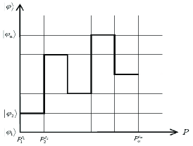
Figure 4: The consistent history in the state-operator lattice space. There exist $n$ eigenstates within the scope, and the number of the projection (activer) $\alpha$ represents the evolve of time. When the states become continuum, the lattice space becomes continuous space. The black polylines stands for the consistent history.

Kraus Operator for open system Kraus . We study via the widely concerned model of the pure universe wang ; Popescu . Let universe $\mathcal{U}$ be composed with system $\mathcal{S}$ and environment $E$, labeled as $\mathcal{U}=\mathcal{S}+E$. The initial state is $|\psi_{S}(0)\rangle$ and $|\psi_{E}(0)\rangle$, correspondingly, the initial state for the universe is thus $|\psi(0)\rangle=|\psi_{S}(0)\rangle|\psi_{E}(0)\rangle$. The evolution of the wave function is $|\psi(t)\rangle=U(t)|\psi(0)\rangle$, with the evolution operator $U(t)$. The reduced density matrix for the system is

$$\rho_{S}(t) = \textrm{Tr}_{E}|\psi(t)\rangle\langle\psi(t)|$$

$$= \sum_{i}\langle i|U(t)|\psi_{S}(0)\rangle|\psi_{E}(0)\rangle\langle\psi_{S}(0)|\langle\psi_{E}(0)|U^{\dagger}(t)|i\rangle$$

$$= \sum_{i}K_{i}(t)\rho_{S}(0)K^{\dagger}_{i}(t),$$

where $\rho_{S}(0)=|\psi_{S}(0)\rangle\langle\psi_{S}(0)|$, $K_{i}(t)=\langle i|U(t)|0\rangle$, and we let $|\psi_{E}(0)\rangle=|0\rangle$. The normalization rule is

$$\sum_{i}\langle 0|U^{\dagger}(t)|i\rangle\langle i|U(t)|0\rangle=1.$$ (61)

The Kraus operator representation demonstrates the openness and the evolution in time of quantum system. However, although there is evolution in time, the logical relations between operators remains. For instance, the relation $\sum_{i}K_{i}^{\dagger}K_{i}=1$ does not depends on time. Below, we show that this method is consistent with the CH method.

The physical role of the evolution operator $U(t)$ can be substituted by the class operator $\mathcal{C}_{\alpha}$, the state of the system at time $t_{n}$ is $|\psi_{S}(t_{n})\rangle=\mathcal{C}_{\alpha}|\psi_{S}(0)\rangle$, where $|\psi_{S}(0)\rangle$ is the initial state. We know

$$\mathcal{D}(\alpha)=\textrm{Tr}(\mathcal{C}_{\alpha}|\psi(0)\rangle\langle\psi(0)|\mathcal{C}^{\dagger}_{\alpha}),$$ (62)

and

$$\sum_{\alpha}\mathcal{D}(\alpha) = \sum_{\alpha}\textrm{Tr}\mathcal{C}_{\alpha}|\psi(0)\rangle\langle\psi(0)|\mathcal{C}^{\dagger}_{\alpha}$$

$$= \textrm{Tr}\sum_{\alpha}\mathcal{C}_{\alpha}|\psi(0)\rangle\langle\psi(0)|\mathcal{C}^{\dagger}_{\alpha}$$

$$= \textrm{Tr}\sum_{\alpha}\mathcal{C}_{\alpha}\rho_{S}(0)\mathcal{C}^{\dagger}_{\alpha}$$

$$= 1,$$

thus $\sum_{\alpha}\mathcal{C}_{\alpha}\mathcal{C}_{\alpha}^{\dagger}=1$, which is the same as the normalization of the Kraus operator, physically.

Interacting Faculties. The concept of “potentiality”, originated from Aristotle Aristotle , is quite widely studied in QM. The actuality (reality) and potentiality were systematically studied recently, where the authors stated that potentiality could be a mode of existence, and the concept of “faculty” was introduced to replace “entity” Ronde . The faculty describes a level which does not pertain to things but rather to potential actions. Possessing a faculty offers the ability to do something. According to our understanding, yet, the concept of faculty is the analogy of potentiality. This approach relates to the property $4$ in section III.2, yet it does not aim to provide the direct physical meaning of wave function and the superposition principle.

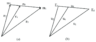
Figure 5: The models for the two-body problem in CM (a) and the mixtures of qubit in QM. The meaning for the symbols is explained in the text.

Appendix C Reduced entanglement

Consider the mixtures of Bell states $|\Psi\rangle=(|01\rangle\pm|10\rangle)/\sqrt{2}$, $|\Phi\rangle=(|00\rangle\pm|11\rangle)/\sqrt{2}$. According to our definition, the state $|\Psi\rangle$ is the “cross” state, and $|\Phi\rangle$ is the “direct” state. So the mixture (ensemble) can be viewed as the mixture of two kinds of systems. The classical analogy is, e.g., the mixture of two kinds of gases. There exists the center of mass for each of the gases, so the problem can be simplified as the two-body problem in classical mechanics, as shown in Fig. 5(a). The two objects $m_{1}$ and $m_{2}$ exist in the configuration space, the coordinates are ${\bf r_{1}}$ and ${\bf r_{2}}$, respectively. The kinetic energy is

$$E_{k} = \frac{1}{2}(m_{1}\dot{{\bf r}}_{1}^{2}+m_{2}\dot{{\bf r}}_{2}^{2})$$

$$= \frac{1}{2}(M\dot{{\bf r}}_{c}^{2}+\mu\dot{{\bf r}}_{0}^{2}),$$

where $M=m_{1}+m_{2}$ is the total mass, $\mu=\frac{m_{1}m_{2}}{m_{1}+m_{2}}$ is the reduced mass, ${\bf r_{c}}=\frac{m_{1}{\bf r_{1}}+m_{2}{\bf r_{2}}}{m_{1}+m_{2}}$ is the coordinate of the mass center of the system, and ${\bf r_{0}}={\bf r_{1}}-{\bf r_{2}}$ is the relative displacement between the two objects.

Now, consider velocity ${\bf v}=\dot{{\bf r}}$. As we know, there exists the maximum speed as the light speed $c$. Let $c=1$, thus, the set of speed $v=|{\bf v}|/c$ forms the probability space with $0\leqslant v\leqslant 1$. The kinetic energy is written as

$$E_{k}=\frac{1}{2}(Mv_{c}^{2}+\mu v_{0}^{2}).$$ (65)

Consider the mixtures of Bell states. The density matrix can be written as

$$\rho=p_{1}|\Phi\rangle\langle\Phi|+p_{2}|\Psi\rangle\langle\Psi|.$$ (66)

The entanglement of the mixture is

$$\mathcal{E}_{\rho} = p_{1}\mathcal{E}_{d}+p_{2}\mathcal{E}_{c}$$

$$= (\mathcal{E}_{d}+\mathcal{E}_{c})p_{c}+\frac{\mathcal{E}_{d}\mathcal{E}_{c}}{\mathcal{E}_{d}+\mathcal{E}_{c}}p_{0},$$

where by introducing the probability amplitude $u=\sqrt{p}$, $u_{c}=\frac{u_{1}\mathcal{E}_{d}+u_{2}\mathcal{E}_{c}}{\mathcal{E}_{d}+\mathcal{E}_{c}}$, $u_{0}=|u_{1}-u_{2}|$, and $\frac{\mathcal{E}_{d}\mathcal{E}_{c}}{\mathcal{E}_{d}+\mathcal{E}_{c}}\equiv\mathcal{E}^{\dagger}$ is the reduced entanglement. The situation is depicted in Fig. 5(b).

By comparison, the entanglement is the analogy of mass, the probability is the analogy of $v^{2}$.

For high-dimensional and many-body problems, there is no obvious form of reduced mass, also the reduced entanglement. Yet, we can apply the rough bi-party partition to deduce the apparent reduced mass or entanglement.

However, we have to say, there are significant differences. For instance, the quantum probabilities $p_{1}$ and $p_{2}$ each exist in the probability space, and also they together exist in another probability space. But, the classical speed (square) $v_{1}^{2}$ and $v_{2}^{2}$ do not exist in the probability space with each other. This relates to the problem of Special Relativity, this simple mode may have implication for the relation between QM and Relativity.

Appendix D Entanglement measure

According to our study, entanglement and quantum information (entropy) are different. Entanglement is the shared coherence by the parties of the entangled state. Also, we find nonorthogonality is the shared coherence within the local states of each party of the whole state. Quantum information ($\mathcal{I}_{q}$) is the improved form of classical information (correlation) ($\mathcal{I}_{c}$) due to nonorthogonality ($\bar{\mathcal{O}}$) or entanglement ($\mathcal{E}$). Thus, $\mathcal{I}_{q}$ can be the function of $\bar{\mathcal{O}}$ or entanglement $\mathcal{E}$. Here, we compare our definition with the usual entanglement measure.

Entanglement of formation. In QIQC, the mixtures of Bell states, i.e., ensemble of qubits, are often prepared, the entanglement of formation, also cost and distillation are studied bbps ; Hill ; Bennett . The entanglement of formation, which measures quantum information instead of entanglement, is defined as

$$E_{f}(\rho)=\textrm{min}\sum_{i}^{n}p_{i}E(\psi_{i}),$$ (68)

and the density matrix is written as $\rho=\sum_{i}^{n}p_{i}|\psi_{i}\rangle\langle\psi_{i}|$. This decomposition is the ensemble of entangled qudit. Here we prove one simple property of $E_{f}(\rho)$ as follows.

When the density matrixes $\omega$, $\sigma$, and $\rho$ satisfying

$$\omega = r_{1}\rho+r_{2}\sigma$$

$$= r_{1}\sum_{i=1}^{i=n}p_{i}|\psi_{i}\rangle\langle\psi_{i}|+r_{2}\sum_{j=1}^{j=m}q_{j}|\phi_{j}\rangle\langle\phi_{j}|$$

$$= \sum_{i=1}^{i=n}r_{1}p_{i}|\psi_{i}\rangle\langle\psi_{i}|+\sum_{i=n+1}^{i=n+m}r_{2}q_{i}|\phi_{i}\rangle\langle\phi_{i}|.$$

The entanglement of formation of $\omega$ is

$$E_{f}(\omega) = \textrm{min}(r_{1}\sum_{i=1}^{i=n}p_{i}E(\psi_{i})+r_{2}\sum_{i=n+1}^{i=n+m}q_{i}E(\phi_{i}))$$ (70)

$$= r_{1}E_{f}(\rho)+r_{2}E_{f}(\sigma).$$

Concurrence. Concurrence relies on the permutation symmetry of entangled state Werner89 . For pure state, concurrence describes the coherence. There are three kinds of basis to express the qubit.

(a). “Magic basis” $\{|e_{i}\rangle\}$ Hill . The qubit is written as $|\psi\rangle=\sum_{i}\alpha_{i}|e_{i}\rangle=(\alpha_{1}+i\alpha_{2},i\alpha_{3}+\alpha_{4},i\alpha_{3}-\alpha_{4},\alpha_{1}-i\alpha_{2})^{T}/2.$ Concurrence is

$$C=|\sum_{i}\alpha_{i}^{2}|=\alpha_{1}^{2}+\alpha_{2}^{2}+\alpha_{3}^{2}+\alpha_{4}^{2}.$$ (71)

(b). “Computation basis” $|00\rangle$, $|01\rangle$, $|10\rangle$, $|11\rangle$. The qubit is written as $|\psi\rangle=(a,b,c,d)^{T}$, and concurrence is

$$C=2|ad-bc|.$$ (72)

It is easy to see that the basis in case (a) can be viewed as the special case of (b).

(c). Schmidt basis $|ii\rangle$. The qubit is written as $|\psi\rangle=x|00\rangle+y|11\rangle$, with $x^{2}+y^{2}=1$, the density matrix is

$$\rho=\left(\begin{array}[]{cccc}x^{2}&0&0&xy\\ 0&0&0&0\\ 0&0&0&0\\ xy&0&0&y^{2}\end{array}\right),$$ (73)

and concurrence is

$$C=2|xy|.$$ (74)

The Schmidt basis can be rotated to the “computation basis” in case (b) by the local unitary transformation $U_{A}\otimes U_{B}$ Abouraddy .

The above three kinds of basis give the same results of concurrence. The entanglement of formation is defined as $E_{f}=h(\frac{1+\sqrt{1-C^{2}}}{2})$, where the binary entropy function $h(x)=-x\log_{2}x-(1-x)\log_{2}(1-x)$. We can form the entropy-concurrence matrix ($\Lambda$) as follows

$$\Lambda=\frac{1}{2}\left(\begin{array}[]{cc}1+\sqrt{1-C^{2}}&C\\ C&1-\sqrt{1-C^{2}}\end{array}\right).$$ (75)

Then, it is obvious that the entropy $E_{f}$ describes the property of the diagonal elements (population), and the concurrence $C$ describes the non-diagonal elements (coherence).

Negativity and Robustness. For pure state, the definition of negativity Vidal02 is the same with our definition of the degree of entanglement. Negativity is usually viewed as the absolute value of the sum of the negative eigenvalues of $\rho^{T_{A}}$

$$\mathcal{N}=\frac{||\rho^{T_{A}}||_{1}-1}{2}=|\sum_{i}\mu_{i}|,$$ (76)

where $\mu_{i}$ is the negative eigenvalues.

In deed, the negative eigenvalues are the results of the shared coherence of the entangled state. For pure qubit, the negativity is the same with concurrence, that is to say, the definition of negativity is more general than concurrence for bi-party pure state.

The robustness Vidal99 is the twice of the negativity for pure state. Physically, it describes the robustness of the entanglement to the minimal amount of external classical noise. The role of noise is to disturb and destroy the coherence. Physically, the robustness can describe the shared coherence, thus give the right quantity of entanglement. However, it is not easy to calculate since it is the indirect way to measure entanglement.

In addition, we discuss a little of the physical meaning of concurrence and negativity for the mixed state condition. It is well-known that the two are often different for mixed state, though the same for the pure state case. The physical reason is quite clear: they are the results of two different entanglement witness (operator) Brandao . Physically, in the mixed state there can be nonorthogonality, which can influence concurrence and negativity without being detected. That is to say, it is not proper to generalize concurrence and negativity to the mixed state, since the result is not necessarily entanglement.

Relative entropy. The quantum relative entropy of entanglement Vedral is defined as

$$E_{r}(\rho) = \inf_{\sigma\in X}S(\rho||\sigma)$$

$$= \inf_{\sigma\in X}\textrm{tr}(\rho\log\rho-\rho\log\sigma),$$

where the set $X$ can be taken as the set of separable states, states with positive partial transpose, nondistillable states, etc. The quantum discord Ollivier ; Luo and squashed entanglement Christandl , which we have studied in Ref. wang , can be viewed as the relative entropy.

Physically, $E_{r}$ does not quantify entanglement directly, yet it relates to entanglement. The relation between $E_{r}$ and entanglement also nonorthogonality can not be deduced easily especially for mixed state, since the detailed structure of the mixed state and the distribution of coherence are not clear. As a result, the relative entropy is only an effective way to measure quantum information instead of entanglement.

References

- (1) D. Bohm, Quantum Theory (Prentice-Hall, Inc., Englewood Cliffs, New Jersey, 1951).
- (2) M. Jammer, The Philosophy of Quantum Mechanics (Wiley, New York, 1974).
- (3) J. S. Bell, Speakable and Unspeakable in Quantum Mechanics (Cambridge University Press, Cambridge, England, 1987).
- (4) M. A. Nielsen and I. L. Chuang, Quantum Computation and Quantum Information (Cambridge University Press, Cambridge, England, 2000).
- (5) W. H. Zurek, Rev. Mod. Phys. 75, 715 (2003).
- (6) M. Schlosshauer, Rev. Mod. Phys. 76, 1267 (2004).
- (7) C. G. Timpson, arXiv:quant-ph/0611187.
- (8) R. F. Werner and M. M. Wolf, arXiv:quant-ph/0107093; A. J. Leggett, Found. Phys. 33, 1469 (2003). N. Gisin, arXiv:quant-ph/0702021.
- (9) A. Einstein, B. Podolsky, and N. Rosen, Phys. Rev. 47, 777 (1935).
- (10) E. Schrödinger, Phys. Rev. 28, 1049 (1926).
- (11) D. Bohm, Phys. Rev. 85, 166 (1952).
- (12) J. von Neumann, Mathematical Foundations of Quantum Mechanics (Princeton University Press, 1955).
- (13) H. Everett, Rev. Mod. Phys. 29, 454 (1957); B. S. DeWitt and N. Graham, The Many Worlds Interpretation of Quantum Mechanics (Princeton University Press, Princeton NJ, 1973); D. Deutsch, Int. J. Theor. Phys. 24, 1 (1985).
- (14) H. D. Zeh, Found. Phys. 1, 69 (1970); 3, 109 (1973).
- (15) L. E. Ballentine, Rev. Mod. Phys. 42, 358 (1970).
- (16) P. Pearle, Phys. Rev. D 13, 857 (1976); N. Gisin, Phys. Rev. Lett. 52, 1657 (1984); G. C. Ghirardi, A. Rimini, and T. Weber, Phys. Rev. D 34, 470 (1986).
- (17) M. Gell-Mann and J. B. Hartle, in Complexity, Entropy and the Physics of Information, Santa Fe Institute Studies in the Science of Complexity Vol. VIII edited by W. Zurek (Addison-Wesley, Redwood City, CA, 1990); Phys. Rev. D 47, 3345 (1993); R. B. Griffiths, J. Stat. Phys. 36, 219 (1984); R. Omnés, Rev. Mod. Phys. 64, 339 (1992); H. F. Dowker and J. J. Halliwell, Phys. Rev. D 46, 1580 (1992); J. J. Halliwell, Phys. Rev. D 58, 105015 (1998); Phys. Rev. Lett. 83, 2481 (1999).
- (18) J. G. Cramer, Rev. Mod. Phys. 58, 647 (1986).
- (19) B. van Fraassen, Quantum Mechanics: An Empiricist View (Clarendon, Oxford, 1991).
- (20) N. D. Mermin, Pramana 51, 549 (1998); Am. J. Phys. 66, 753 (1998).
- (21) C. Dewdney, G. Horton, M. M. Lain, Z. Malik, and M. Schraidt, Found. Phys. 22, 1217 (1992).
- (22) Y. Aharonov and L. Vaidman, arXiv:quant-ph/0105101.
- (23) D. Aerts, arXiv:quant-ph/1005.3767.
- (24) C. de Ronde, arXiv:quant-ph/0711.4738.
- (25) C. Jansson, arXiv:quant-ph/0802.3625.
- (26) L. Hardy, arXiv:quant-ph/0101012; arXiv:quant-ph/ 1005.5164.
- (27) C. M. Caves, C. A. Fuchs, and R. Schack, Phys. Rev. A 65, 022305 (2002).
- (28) S. Popescu and D. Rohrlich, Found. Phys. 24, 379 (1994); J. Barrett, Phys. Rev. A 75, 032304 (2007); N. Gisin, Science 326, 1357 (2009).
- (29) R. Clifton, J. Bub, and H. Halvorson, Found. Phys. 33, 1561 (2003); G. Brassard, Nature Phys. 1, 2 (2005); J. Oppenheim and B. Reznik, arXiv:quant-ph/0312149; G. M. D’Ariano, arXiv:quant-ph/1012.0535; Jae-Weon Lee, arXiv:hep-th/1011.1657; P. Goyal, arXiv:quant-ph/0702124; arXiv:quant-ph/0702149.
- (30) A. Ashtekar and T. A. Schilling, arXiv:gr-qc/9706069.
- (31) N. N. Gorobey and A. S. Lukyanenko, arXiv:quant-ph/0807.3508.
- (32) A. Caulton and J.Butterfield, arXiv:quant-ph/1002.3730.
- (33) B. Z. Iliev, arXiv:quant-ph/9803084.
- (34) A. Döring and C. J. Isham, arXiv:quant-ph/0703062.
- (35) As Bohr said: “There is no quantum world. There is only an abstract quantum physical description. It is wrong to think that the task of physics is to find out how nature is. Physics concerns what we can say about Nature.” From N. Bohr, Atomic Theory and the Description of Nature (Cambridge Univ. Press, New York, 1934).
- (36) D.-S. Wang, arXiv:quant-ph/1101.0503.
- (37) U. Fano, Rev. Mod. Phys. 29, 74 (1957); L. D. Landau and L. M. Lifshitz, Quantum Mechanics (Non-Relativistic Theory) (Butterworth-Heinemann, Oxford, 1981).
- (38) E. Calzetta and F. D. Mazzitelli, Phys. Rev. D 42, 4066 (1990); F. Lombardo and F. D. Mazzitelli, Phys. Rev. D 53, 2001 (1996).
- (39) S. Habib, Y. Kluger, E. Mottola, and J. P. Paz, Phys. Rev. Lett. 76, 4660 (1996); G. Mahajan and T. Padmanabhan, Gen. Rel. Grav. 40, 661 (2008); A. Giraud and J. Serreau, Phys. Rev. Lett. 104, 230405 (2010).
- (40) S. Popescu, A. J. Short, and A. Winter, Nature Phys. 2, 754 (2006); arXiv:quant-ph/0511225.
- (41) J. Cho and M. S. Kim, Phys. Rev. Lett. 104, 170402 (2010).
- (42) E. Schmidt, Math. Ann. 63, 433 (1906).
- (43) E. P. Wigner, Phys. Rev. 40, 749 (1932).
- (44) H. W. Lee, Phys. Rep. 259, 147 (1995).
- (45) P. A. M. Dirac, The Principles of Quantum Mechanics, 4th ed. International Series of Monographs on Physics, Vol. 27 (Oxford University Press, Oxford, England, 1981).
- (46) For the problems of time in physics, please see H. D. Zeh, The Physical Basis of the Direction of Time (Springer, New York, 2001).
- (47) J. Grabowski, M. Kuś, and G. Marmo, arXiv:math-ph/0507045; Jon M. Leinaas, J. Myrheim, and E. Ovrum, Phys. Rev. A 74, 012313 (2006); D. Chruściński, J. Phys.: Conf. Ser. 30, 9 (2006).
- (48) Aristotle, Metaphysics (Oxford, Clarendon Press, 2006).
- (49) W. Heisenberg, Physics and Philosophy (George and Unwin, 1958); H. Margenau, Phys. Today 7(10), 6 (1954).
- (50) B. d’Espagnat, Found. Phys. 35, 1943 (2005).
- (51) D. Wallace, arXiv:quant-ph/0712.0149.
- (52) I. I. Rabi, Phys. Rev. 51, 652 (1937).
- (53) P. G. Kwiat, K. Mattle, H. Weinfurter, A. Zeilinger, A. V. Sergienko and Y. Shih, Phys. Rev. Lett. 75, 4337 (1995).
- (54) R. J. Glauber, Phys. Rev. 131, 2766 (1963); A. Miranowicz et al., Phys. Rev. A 82, 013824 (2010), and references therein.
- (55) G. Vidal, J. Mod. Opt. 47, 355 (2000); M. B. Plenio and S. Virmani, Quantum Inf. Comput. 7, 1 (2007); R. Horodecki, P. Horodecki, M. Horodecki, and K. Horodecki, Rev. Mod. Phys. 81, 865 (2009).
- (56) A. Aspect, J. Dalibard, and G. Roger, Phys. Rev. Lett. 49, 1804 (1982).
- (57) C. H. Bennett and G. Brassard, Proceedings of the IEEE International Conference on Computers, Systems and Signal Processing (IEEE Computer Society, New York, 1984), pp. 175-179.
- (58) C. H. Bennett, Phys. Rev. Lett. 68, 3121 (1992).
- (59) F. Grosshans et al., Nature 421, 238 (2003).
- (60) H.-K. Lo, X. Ma, K. Chen, Phys. Rev. Lett. 94, 230504 (2005).
- (61) E. Knill and R. Laflamme, Phys. Rev. Lett. 81, 5672 (1998).
- (62) A. Datta, arXiv:quant-ph/0807.4490.
- (63) J. Barrett, L. Hardy, and A. Kent, Phys. Rev. Lett. 95, 010503 (2005).
- (64) J. A. Wheeler and K. Ford, Geons, black holes quantum foam: a life in physics (New York: W.W. Norton Co, 1998).
- (65) J. A. Wheeler, In W. Zurek, editor, Complexity, Entropy and the Physics of Information, pages 3-28. (Addison-Wesley, Redwood City, CA 1990).
- (66) R. Landauer, Proc. Workshop on Physics and Computation PhysComp ’92 (IEEE Comp. Sci. Press, Los Alamitos, 1993) pp. 1-4.
- (67) A. Zeilinger, Found. Phys. 29(4), 631 (1999); Q. Schiermeier, Nature 434, 1066 (2005); M. Arndt et al., arXiv:quant-ph/0505187.
- (68) R. F. Werner, Phys. Rev. A 40, 4277 (1989).
- (69) D. M. Greenberger, M. A. Horne, and A. Zeilinger, Going Beyond Bell’s Theorem in Bell’s Theorem, and Conceptions of the Universe (Kluwer Academic, Dordrecht, 1989); Phys. Today 8, 22 (1993); D. M. Greenberger, M. A. Horne, A. Shimony, and A. Zeilinger, Am. J. Phys. 58, 1131 (1990).
- (70) A. Peres, Phys. Rev. Lett. 77, 1413 (1996).
- (71) G. Vidal and R. F. Werner, Phys. Rev. A 65, 032314 (2002).
- (72) C. H. Bennett, H. J. Bernstein, S. Popescu, B. Schumacher, Phys. Rev. A 53, 2046 (1996).
- (73) S. Hill and W. K. Wootters, Phys. Rev. Lett. 78, 5022 (1997); W. K. Wootters, Phys. Rev. Lett. 80, 2245 (1998).
- (74) C. H. Bennett, D. P. DiVincenzo, J. A. Smolin, and W. K. Wootters, Phys. Rev. A 54, 3824 (1996).
- (75) V. Vedral and M. B. Plenio, Phys. Rev. A 57, 1619 (1998)
- (76) G. Vidal and R. Tarrach, Phys. Rev. A 59, 141 (1999).
- (77) M. Steiner, Phys. Rev. A 67, 054305 (2003).
- (78) H. Ollivier and W. H. Zurek, Phys. Rev. Lett. 88, 017901 (2001); W. H. Zurek, Phys. Rev. A 67, 012320 (2003); L. Henderson and V. Vedral, J. Phys. A 34, 6899 (2001).
- (79) S. Luo, Phys. Rev. A 77, 022301 (2008).
- (80) M. Christandl and A. Winter, J. Math. Phys.(N.Y.) 45, 829 (2004).
- (81) F. G. S. L. Brandão, Phys. Rev. A 72, 022310 (2005).
- (82) O. Gittsovich, O. Gühne, P. Hyllus, and J. Eisert, Phys. Rev. A 78, 052319 (2008).
- (83) M. Lewenstein and A. Sanpera, Phys. Rev. Lett. 80, 2261 (1998).
- (84) M. Horodecki, P. Horodecki, R. Horodecki, Phys. Rev. Lett. 80, 5239 (1998); L. Pankowski, M. Piani, M. Horodecki, and P. Horodecki, arXiv:quant-ph/0711.2613; R. Simon, arXiv:quant-ph/0608250.
- (85) S. D. Bartlett, T. Rudolph, and R. W. Spekkens, Rev. Mod. Phys. 77, 555 (2007).
- (86) L. de Broglie, An Introduction to the Study of Wave Mechanics (E. P. Dutton and Co., New York, 1930); L. de Broglie, J. Physique (serie 6) VIII (5), 225 (1927).
- (87) K. Kraus, States, Effects and Operations: Fundamental Notions of Quantum Theory (Academic, Berlin, 1983).
- (88) A. F. Abouraddy, B. E. A. Saleh, A. V. Sergienko, and M. C. Teich, Phys. Rev. A 64, 050101(R) (2001).