Robustness of Estimators of Long-Range Dependence and Self-Similarity under non-Gaussianity

Abstract

Memory, Paradigmatic Models, Multiplicative Noise Long-range dependence and non-Gaussianity are ubiquitous in many natural systems like ecosystems, biological systems and climate. However, it is not always appreciated that both phenomena may occur together in natural systems and that self-similarity in a system can be a superposition of both phenomena. These features, which are common in complex systems, impact the attribution of trends and the occurrence and clustering of extremes. The risk assessment of systems with these properties will lead to different outcomes (e.g. return periods) than the more common assumption of independence of extremes.

Two paradigmatic models are discussed which can simultaneously account for long-range dependence and non-Gaussianity: Autoregressive Fractional Integrated Moving Average (ARFIMA) and Linear Fractional Stable Motion (LFSM). Statistical properties of estimators for long-range dependence and self-similarity are critically assessed. It is found that the most popular estimators can be biased in the presence of important features of many natural systems like trends and multiplicative noise. Also the long-range dependence and non-Gaussianity of two typical natural time series are discussed.

1 Introduction

Meteorology has been both a seedbed and a testbed for many advances in the mathematics of complex systems; the former being seen in its contribution of the Lorenz model to nonlinear science (Lorenz 1963), while the latter is exemplified by ensemble forecasting. This parallel evolution of theory and practise has identified important problems, e.g., the need to model the effect of extra, noise-like, degrees of freedom on deterministic low dimensional dynamics. Other well established paradigms such as Hasselmann’s stochastic model (Hasselmann 1976), have highlighted the importance of red noise to mathematical climatology.

However, since the pioneering work of the late Benoit Mandelbrot, increasing attention is paid to two self-similar (or “fractal”) aspects of time series: long-range dependence (LRD) in time, and the spatial counterpart of LRD, heavy tailed probability distributions in amplitude. First identified in hydrology, and since studied in research areas as diverse as biology, telecommunications, social networks, econometrics and the climate system, LRD is characterised by its low frequency singular behaviour, the so-called $1/f$ power spectrum. When present in a signal the correlations captured by LRD will both hamper the identification and the attribution of deterministic trends (e.g. Franzke 2010), and impede the quantification of their significance. As was the case in the original context of hydrology, the presence of LRD in climate time series has been intensely debated, and it is still sometimes ascribed to transient effects, calibration issues or other forms of nonstationarity (Maraun et al. 2004, Rust et al. 2008).

LRD is also of practical significance. By making systems subject to longer-lived fluctuations (Beran 1994) it changes the information available to make predictions about the state of a complex system. It impacts the occurrence and clustering of extremes (Bunde et al. 2005, Bogachev et al. 2008, Kropp and Schellnhuber 2010) which are important for risk assessments and mitigation strategies, e.g. insurance pricing and flood defence. The traditional assumption is that extremes are independent events. But there is growing evidence for clustering of extreme extra-tropical storms (e.g. Mailier et al. 2006) and precipitation events (e.g. 2007 United Kingdom floods). This clustering of extremes will lead to higher return periods of extreme events than the more common assumption of independence. Recently, detrended fluctuation analysis (DFA), a tool originally developed to detect LRD, has found application in the prediction of dangerous bifurcations in dynamical systems such as climate “tipping points” (Livina and Lenton 2007, Lenton et al. 2011, Sieber and Thompson 2011). Our contribution to this volume is focused both on i) the problem of accurately estimating LRD in the presence of other signal elements, and ii) the complicating effects of heavy-tailed amplitude distributions, when they are present.

A process is long range dependent when the prediction of its next state depends on the whole of its past. An imprint of this dependence structure is that the covariance $\ r(k)=Cov(X(k),X(0))$ decays slowly, as$\ k\rightarrow\infty$, so that

$$\sum_{k=0}^{\infty}|r(k)|=\infty.$$ (1)

This slow decay of the covariances means that the values of the process X are strongly dependent over long periods of time. This contrasts with the more familiar short-range dependent system where $\sum_{k=0}^{\infty}|r(k)|=C<\infty$. In a short-range dependent process the next state only depends on the current state and the recent past. The archetype of a short-range dependent process is a first order Markov process where the next state depends only on the present state and is conditionally independent of past states. See Beran (1994) for more details.

Long-range dependence of a system is characterised by the parameter $d$ in the statistics literature and sometimes by Mandelbrot’s Joseph parameter $J$, for example in the physics literature. Temporal long-range dependence has been detected in the water level of the river Nile (Hurst 1951, Hurst et al. 1965). It was observed that the range of values grows as $\tau^{J}$, where $J$ refers to the Joseph exponent (e.g. Mandelbrot 2001, p. 157) and $\tau$ to the time period under consideration. The growth of range was anomalously large compared to that in the familiar paradigms of random walks and Brownian motion, which have both played a central role in understanding diffusion. In the random walk, the variance grows as the square root of time $\tau^{1/2}$ (Einstein 1905). The subsequent theoretical explanation of the difference between the observed anomalous diffusion and the Brownian motion paradigm came first through the use of a self-similar process, in particular via the study of fractional Brownian motion (fBm; Mandelbrot & Wallis 1968). Here, self-similarity means that the statistical properties on all scales are similar. This property is controlled by the self-similarity parameter $H$. A stochastic process $S$ is self-similar when a rescaling of time by a factor $\lambda$ leads to a rescaling of the amplitude of the process $S$ by $\lambda^{H}$. Thus, a process is said to be $H$-self-similar when the following relation holds (Embrechts and Maejima 2002):

$$S(\lambda t)\stackrel{{\scriptstyle d}}{{\sim}}\lambda^{H}S(t).$$ (2)

where $\stackrel{{\scriptstyle d}}{{\sim}}$ denotes equality in distribution. It is not always appreciated, and is sometimes confused in the literature, that two different aspects of a time series can contribute to its self-similarity $H$. The first is LRD, which is synonymous with persistence, referred to by Mandelbrot and Wallis (1968) as the Joseph effect. Persistent systems exhibit longevity by having a tendency to maintain the way they have been recently. Examples are heat waves and drought conditions. The second source of self-similarity identified by Mandelbrot, the so-called Noah effect is the property that change in a system can be rather large and can occur very abruptly i.e. time series drawn from systems can exhibit sharp discontinuities, e.g., Earth quakes.

It may at first seem odd that both phenomena occur simultaneously in natural systems because they pull in opposite directions. On reflection, taken together, however, we see that the two effects capture the facts that coherent structures in nature are real and that they can emerge, change or even vanish very quickly. The archetypal model of the Noah effect is non-Gaussian jumps whose complementary cumulative distribution function decays with a power law in size $s$, $p(s)\sim s^{-\alpha}$. Here, $\alpha$ denotes the stability exponent (referred to as tail exponent in the statistics literature). Thus, the self-similarity parameter is

$$H=J-\frac{1}{2}+\frac{1}{\alpha}=d+\frac{1}{\alpha},\quad H\in(0,1).$$ (3)

The distinction between $H$ and $J=d+\frac{1}{2}$ is important because not all observed time series have Gaussian fluctuations. As such one may find that popular diagnostics, as shown below, may be insensitive to heavy tails, measuring J and not H. However, in many situations both heavy tails and the clustering of extremes caused by LRD are very important and both contribute to the value of H. This makes it necessary to be able to measure both H and J independently.

Many estimators for the LRD exponent $d$ have thus been developed, and are widely used in the respective literatures. Much of what has been rigorously established about the estimators, however, is for a particular LRD Gaussian model: fBm, which is also $H$ self-similar and has a particularly simple relation between $H$ and $J$, i.e. $H=J+\frac{1}{2}-\frac{1}{2}=J$ ($\alpha=2$ for Gaussian increments). Most observed time series depart from the assumptions of fBm in some way or another, so it is important to critically evaluate how sensitive the estimators are to deviations from fractional Gaussian noise (fGn). fBm is a random walk with long-range correlated increments and the value of $J$ in such $H$-self-similar walks is directly connected to the presence of LRD in their increments.

In this study we critically re-evaluate 4 popular methods for measuring $d$ and two for measuring $H$: variable bandwidth estimator (Schmittbuhl et al. 1995) and wavelets (WL; Stoev and Taqqu 1995), Detrended Fluctuation Analysis (DFA; Peng et al. 1994), the Re-Scaled Range analysis ($R/S$; Hurst 1951, Mandelbrot 2001), exact Whittle estimator (Shimotsu and Phillips 2005, 2006) and semi-parametric estimators (in this study we will focus on the Geweke-Porter-Hudak (GPH) estimator; Geweke & Porter-Hudak 1983; semi-parametric estimators are also described in Bardet et al. 1998, Robinson 1995a, 1995b, Hurvich et al. 2005). This is a not a complete set of estimators for the self-similarity or long-range dependence parameter (other estimators, which are well established in the statistics community include FEXP (Hurvich et al. 2002)). Here we want to focus on some of the most popular estimators in the physics and geosciences communities ($R/S$: Tuck and Hovde 1999, Price and Newman 2001, Ogurtsov, 2004, Scipioni et al, 2008, Ghil et al. 2011, DFA: Chen et al. 2002, Bunde et al. 2005, Bashan et al. 2008, Ghil et al (2011), GPH: Vyushin and Kushner 2009, Huybers and Curry 2006, Franzke 2010, $\mathrm{VB}$: Escorcia-Garcia et al. 2009, WL: Stoev and Taqqu 2005, Stoev et al. 2005).

We show scatter plots which compare the imposed parameters for a number of trials with the values detected by the above methods. These have the advantage of visually indicating which methods measure the complete self-similarity exponent $H$, and which, instead, measure long range dependence via $d$. For evaluating the performance of these estimators we employ 2 well-established paradigmatic time series models: A self-similar process (Linear Fractional Stable Motion (LFSM); Samorodnitsky & Taqqu 1994) and an asymptotically self-similar process (Autoregressive Fractional Integrated Moving Average (ARFIMA); e.g. Beran 1994).

In most natural systems trends are common properties, so we systematically examine the performance of the various estimators when a linear trend is superposed on each time series. This is an important issue because in practice it is not always easy to remove trends. That they typically manifest themselves in higher moments presents further challenges still. Trends are the hardest to deal with because long-range dependent processes can produce apparent trends over rather long periods of time (e.g. Franzke 2010). Therefore, it can be difficult to decide if a trend is due to external forcing or due to finite time series length.

In section 2 we present the two paradigmatic time series models in more detail and discuss various special cases. In section 3 we introduce the estimators of long-range dependence and self-similarity. We test their utility in section 4. In section 5 we discuss the LRD and self-similarity properties of two exemplary time series from nature and in section 6 we provide conclusions.

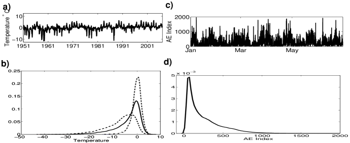
Figure 1: a) Faraday-Vernadsky station temperature time series in degree Celsius (annual cycle is subtracted) (01.01.1951 - 28.02.2007), b) Probability density function of the Faraday-Vernadsky station temperature time series estimated by a Kernel density estimator: Solid line: whole year; Dashed line: Cold season data May through September; Dashed-Dotted line: Warm season data November through March. c) Auroral electrojet index from January through June 2006 in nanotesla and d) Probability density function of the Auroral electrojet index.

2 Paradigmatic Models of Natural Time Series

2.1 Natural Time Series Examples

The most prominent and widely used paradigmatic LRD time series model, especially in the physics literature, is fGn. However, most natural time series are not strictly Gaussian and many are actually highly non-Gaussian. To illustrate this point we discuss two time series from nature. In Fig. 1a we display monthly mean temperature from the Antarctic station Faraday-Vernadsky (Turner et al. 2004, Franzke 2010). It is easy to see that the raw time series is highly non-Gaussian. This is confirmed by the probability distribution functions (PDFs) plotted in Fig. 1b. There is also a striking seasonal signal visible in the skewness of the PDFs. However, it must to be noted that polar temperature time series are much more non-Gaussian than mid-latitude ones which are typically nearly Gaussian. Our second exemplary time series is the auroral electrojet (AE) index (Fig. 1, e.g., Davis & Sugiura 1966, Watkins 2002). The AE index is derived from 1 minute resolution time series from 12 high latitude magnetometers. Reflecting the intermittent nature of the ionospheric and solar wind processes which influence it, the AE index is seen to be spiky and strongly non-Gaussian (Fig. 1d). Clearly, many natural time series are non-Gaussian.

2.2 Paradigmatic Models

While fGn and fBm are Gaussian, they are still useful idealised paradigmatic models for understanding many observed phenomena. A paradigmatic model is an idealised framework which captures some properties of observed time series, though not all. Most paradigmatic models allow analytical work, although at the expense of an over-idealisation of the physical or biological phenomena. There is a need for better paradigmatic models of observed phenomena which allow simultaneously non-Gaussian statistics and LRD. Such models are needed e.g., for hypothesis testing and time series simulation. Thus, we briefly discuss two paradigmatic time series models which exhibit LRD and non-Gaussianity. The widely used fGn and fBm are special cases in the Gaussian limit of these more general models, thereby retaining some of the analytical tractability of these models.

In this study we use two classes of processes with symmetric$\ \alpha$-stable (S$\alpha$S) distributions. They are the LFSM and the ARFIMA model with S$\alpha$S innovations. Stoev and Taqqu (2004) present efficient methods for the simulation of these processes using the Fast Fourier Transform.

2.2.1 Linear Fractional Stable Motion

LFSM is a model which exhibits LRD and heavy tails at the same time. It is an extension to the simpler Brownian random walk model. It links individual heavy tailed jumps by means of a retarded memory kernel. It can be represented by a stochastic process$\ X_{H,\alpha}=\left\{X_{H,\alpha}(t),t\in\mathbb{R}\right\}$, which is defined by the following stochastic integral

$$X_{H,\alpha}(t)=C_{H,\alpha}^{-1}\int_{\mathbb{R}}\left((t-s)^{H-\frac{1}{\alpha}}_{+}-(-s)^{H-\frac{1}{\alpha}}_{+}\right)dL_{\alpha}(s),$$ (4)

where $0<H<1$, $\alpha\in(0,2)$, and where $L_{\alpha}=\left\{L_{\alpha}(s),s\in\mathbb{R}\right\}$ is a standard symmetric $\alpha$-stable (S$\alpha$S) Levy process. The process $\ X_{H,\alpha}$ is called LFSM and is self-similar with self-similarity parameter H. Thus, it satisfies relation (2) and has stationary increments. The parameter $\alpha$ controls the tails of the distribution of an S$\alpha$S random variable $\xi$, that is,

$$\mathbb{P}\left(|\xi|\geq x\right)\sim x^{-\alpha},\mbox{as }x\rightarrow\infty.$$ (5)

The greater the value of$\ \alpha$, the lower the probability of extreme fluctuations of the S$\alpha$S process$\ X_{H,\alpha}$. We recommend the introductions by Taqqu (2003) and Mercik et al. (2003) for detailed expositions.

2.2.2 Fractional Brownian Motion (fBm)

In the Gaussian case we have that $\alpha=2$ and the LFSM process (4) reduces to fBm. In this case the self-similarity parameter $H$ will always equal the Joseph exponent $J$, thus, $H=J=d+\frac{1}{2}$.

2.2.3 Ordinary Lévy Motion (oLm)

In the memory-less case we have $d=0$ and $0<\alpha<2$. In this case equation (5) holds and the tails of the distribution decay according to a power-law and consequently $L_{\alpha}$ has infinite variance and is called ordinary Lévy motion. This encapsulates the Noah effect. In this case the self-similarity exponent is $H=\frac{1}{\alpha}$.

2.2.4 Autoregressive Fractional Integrated Moving Average

Another paradigmatic model exhibiting LRD with heavy-tailed fluctuations is ARFIMA, which has the added ability of exhibiting short-range dependent behaviour. This model, denoted ARFIMA(p,d,q), $p,q\in\mathbb{N}$, extends the usual Autoregressive Integrated Moving Average ARIMA(p,d,q) models, in which $d$ takes integer values (Box & Jenkins 1970). An ARIMA model is written as:

$$\Phi(B)(1-B)^{d}X_{t}=\Psi(B)\epsilon_{t},$$ (6)

where B denotes the back shift operator defined by $BX_{t}=X_{t-1}$,$B^{2}X_{t}=X_{t-2}$… The polynomials $\Phi$ and $\Psi$ are defined as $\Phi(x)=1-\sum_{j=1}^{p}a_{j}x^{j}$ and $\Psi(x)=1+\sum_{j=1}^{q}b_{j}x^{j}$, where p and q are integers. The innovations $\epsilon_{t}~{}(t=1,2...)$ are usually independent and identically distributed (iid) normal variables with zero expectation and variance $\sigma_{\epsilon}^{2}$, but can also be $\alpha$-stable distributed. The widely used autoregressive process of first order (AR(1)) is a special case with $p=1$, $d=0$ and $q=0$. Typically $d$ is an integer. In the case that $d$ is a fractional real number, X(t) is an ARFIMA(p,d,q) process with $-\frac{1}{2}<d<\frac{1}{2}$ and exhibits LRD. In the Gaussian case ARFIMA is stationary. An ARFIMA $(0,d,0)$ is asymptotically equivalent to fBm (Taqqu 2003). An ARFIMA$(p,d,q)$ with $p>0$ and $q>0$ is long-range dependent but not self-similar. However, it is asymptotically self-similar for long time scales.

3 Estimators of Long-Range Dependence and Self-Similarity

Here we briefly describe the four estimators of the self-similarity and LRD parameters used in this study.

3.1 Variable Bandwidth

The variable bandwidth ($\mathrm{VB}$) method (Schmittbuhl et al. 1995) is a technique for estimating the self-similarity exponent, $H$, from a time series $x(t)$. The time series of length $T$ is divided into windows or ‘bands’ of width $r$. The $\mathrm{VB}$ method can deploy two different algorithms to estimate $H$. (i) The standard deviation of the time series, $\sigma(r)$, is computed in each band; or (ii) the difference between the maximum and minimum values in each band, $\epsilon(r)$, is computed. Then $\sigma(r)$ and $\epsilon(r)$ are averaged over all the possible bands by varying the origin at fixed $r$

$$\mathrm{VB}_{w}(r)=\frac{1}{L_{r}}\sum_{i=1}^{L_{r}}\sigma_{i}(r)\mbox{\;\;\;\;\; and \;\;\;\;\;}\mathrm{VB}_{\delta}(r)=\frac{1}{L_{r}}\sum_{i=1}^{L_{r}}\epsilon_{i}(r),$$ (7)

where $L_{r}$ is the number of windows of length $r$. This is repeated over a range of window sizes. Both quantities follow a power-law behaviour for self-similar time series (Schmittbuhl et al. 1995) such that $\mathrm{VB}_{w}(r)=r^{H}$ and $\mathrm{VB}_{\delta}(r)=r^{H}$. Thus, the self-similarity exponent, $H$, is obtained from the slope of the corresponding log-log plot.

3.2 Wavelets

A wavelet $\psi$ is a function with zero average and is normalised to one. A family of wavelets is generated by scaling $\psi$ by a factor $s$ and translating it by $u$ ($\psi_{u,s}(t)=\frac{1}{\sqrt{s}}\psi\left(\frac{t-u}{s}\right)$). The wavelet transform allows to construct a time-frequency representation of a signal, the wavelet spectrum. One can then infer the self-similarity parameter from the wavelet spectrum via ordinary least squares at large wavelet scales (Abry and Veitch 1998, Stoev and Taqqu 2005).

3.3 Rescaled Range

The rescaled range $R/S$ (Hurst 1965) is a technique for estimating the LRD parameter $d$ from a time series. The $R/S$ estimator is given by

$$R/S(\tau)=\frac{\max x(t,\tau)-\min x(t,\tau)}{\sqrt{\frac{1}{\tau}\sum_{t=1}^{\tau}({\xi(t)-\langle\xi\rangle_{\tau}})^{2}}},$$ (8)

where $1\leq t\leq\tau$, $x(t,\tau)=\sum_{u=1}^{t}{x(u)-\langle x\rangle_{\tau}}$, $\langle x\rangle_{\tau}=\frac{1}{\tau}\sum_{t=1}^{\tau}x(t)$. It scales like $\tau^{J}$ where the value of $J$ can be estimated from the slope of $R/S$ from a log-log plot.

3.4 Detrended Fluctuation Analysis

Detrended Fluctuation Analysis (DFA; Peng et al. 1994) also estimates the LRD parameter $d$ from a time series. In DFA, a profile is first computed by $Y(i)=\sum_{t=1}^{N}x(t)$. The profile is cut into $N_{s}$ non-overlapping segments of equal length$\ s$ and then the local trend is subtracted for each segment $v$ by a polynomial least-squares fit of the data. Linear (DFA1), quadratic (DFA2), cubic (DFA3) or higher order polynomials can be used for detrending. In the $n^{th}$ order DFA, trends of order $n$ in the profile, and of order $n-1$ in the original record, are eliminated. Next the variance for each of the$\ N_{s}$ segments is calculated by averaging over all data points$\ i$ in the$\ v^{th}$ segment:

$$F_{s}^{2}(v)=\langle Y_{s}^{2}(i)\rangle=\frac{1}{s}\sum_{i=1}^{s}Y_{s}^{2}\left[(v-1)s+i\right].$$ (9)

Finally, the average over all segments is computed and the square root is applied to obtain the following fluctuation function

$$F(s)=\sqrt{\frac{1}{N_{s}}\sum_{v=1}^{N_{s}}F_{s}^{2}(v)}.$$ (10)

For different detrending orders, $n$, we obtain different fluctuation functions $F(s)$, which are denoted by $F^{(n)}(s)$. The fluctuation function scales according to $F^{(n)}(s)\sim s^{\zeta}$, with $d=\zeta-\frac{1}{2}$. There are many variants of DFA, but use of standard DFA is recommended by Basahn et al. (2008) if the functional form of a trend is not a priori known.

3.5 Exact Whittle Estimator

The Exact Whittle estimator is a semi-parametric estimator (Shimotsu and Phillips 2005, 2006). This method assumes that the underlying model of LRD can be represented by $(1-B)^{d}X_{t}=\varepsilon_{t}$, where $\varepsilon$ is iid noise. See Shimotsu and Phillips (2005, 2006) for more details.

3.6 Power Spectral Method

As a semi-parametric estimator we use the power spectral method of Geweke & Porter-Hudak (1983) and Hurvich et al. (2001). Spectral methods find $d$ by estimating the spectral slope. The periodogram is used, which is an estimate of the spectral density of a finite-length time series and is given by:

$$\hat{S}(\lambda_{j})=\frac{1}{N}\left|\sum_{t=1}^{N}X(t)e^{-i2\pi t\lambda_{j}}\right|^{2},\quad j=1,...,[N/2],$$ (11)

where$\ \lambda_{j}=j/N$ is the frequency and the square brackets denote rounding towards zero. A series with LRD has a spectral density proportional to $\left|\lambda\right|^{-2d}$ close to the origin. Since $\hat{S}(\lambda)$ is an estimator of the spectral density, $d$ is estimated by a regression of the logarithm of the periodogram versus the logarithm of the frequency $\lambda$. Thus having calculated the spectral density estimate $\hat{S}(\lambda)$, semi-parametric estimators fit a power law of the form $f(\lambda,b,d)=b\left|\lambda\right|^{d}$, where $b$ is the scaling factor.

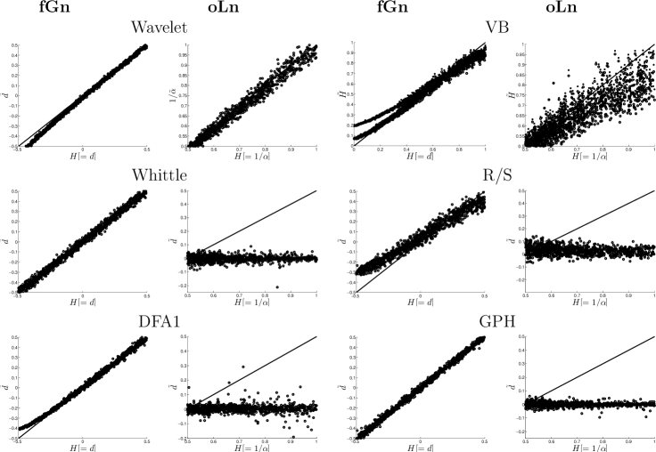
Figure 2: Estimates of $H$ for walks derived from fractional Gaussian noise (fGn) and ordinary Levy noise (oLn) for Wavelet method and the Variable Bandwidth estimator $\mathrm{VB}$ (crosses denote $\mathrm{VB}_{\delta}$ and circles $\mathrm{VB}_{w}$). Estimates of $d$ for fGn and oLn for Whittle estimator, $R/S$, DFA1 and GPH. The solid line indicates the true self-similarity parameter $H$ (d in the case of fGn or $1/\alpha$ for oLn).

4 Empirical Tests

In order to examine the statistical properties of the LRD estimators, like bias, spread and outliers, we generate various test time series from the above paradigmatic models. Specifically, we generate ensembles of 1000 members with randomly selected parameters from uniform distributions: fGn with $d\in(-0.5,0.5)$, oLn with $\alpha\in(1,2)$, ARFIMA with Gaussian increments ARFIMA-G$(1,d,1)$ and with ordinary Levy increments ARFIMA-L$(1,d,1)$ with the autoregressive coefficient $a_{1}\in(-\frac{1}{2},\frac{1}{2})$, and the moving average coefficient $b_{1}\in(0,1)$, $d\in(-\frac{1}{2},\frac{1}{2})$, and $\alpha\in(1,2)$. We also use various first order autoregressive processes with parameters randomly chosen in (-1,1). The time series length is always $2^{15}-M$ with $M=6000$ (see Stoev & Taqqu (2004) for an explanation of $M$) which is comparable to the length of most observed climatic and other natural time series, thus long enough for our purposes.

4.1 Paradigmatic Time Series

First we examine how well the SS and LRD estimators work for the models of self-similarity. Most of the methods (e.g. DFA and $R/S$) require a regression fit in order to estimate the SS or LRD parameters. As shown by Chen et al. (2002) non-stationarities and short-range dependencies can cause crossovers in the fluctuation curves. Because of this we only regress on the long-range part of the fluctuation curves. Our results are robust to the particular choice of the cut off.

As can be seen in Fig. 2 the Wavelet and the $\mathrm{VB}$ methods are the only methods which are able to infer the self-similarity of oLn. While the Wavelet method has no large estimation spread, the $\mathrm{VB}$ method exhibits with large errors. All other estimators estimate $d$ rather than $H$, with $R/S$ producing the largest estimation variance, while Whittle, DFA1 and GPH have considerably smaller estimation variances but with the odd outlier (Fig. 2). All four estimators do a reasonably good job of inferring $H$ from fGn with $\mathrm{VB}_{w}(r)$ having the largest bias for $H$ close to 0 and close to 1, and $R/S$ also having some bias at small $H$ with a relatively large estimation variance. Wavelet, DFA1 and GPH produce very tight estimates, with Wavelet and DFA1 only biased for small values, and Whittle and GPH working well over the entire range. For these paradigmatic time series the two semi-parametric estimators, Whittle and GPH, give the best estimates. This picture changes once we allow for short-term dependence structures to contaminate the pure self-similar character of fGn and oLn. As Fig. 3 shows all estimators work considerably worse for ARFIMA surrogate data with large estimation spreads and many outliers. Again the Whittle estimator and GPH perform better than the other estimators.

Before we go on to examine how well the estimators work with superimposed trends, we test their accuracy on data generated from three basic short-range dependence models: independent white noise, AR(1) and ARFIMA(1,0,1). As Figs. 4a, b and c show, Whittle estimator, GPH and DFA have the least bias. But it also has to be noted that all estimators have many outliers, suggesting that given an individual time series the estimates of $d$ or $H$ can be severely biased. The performance of higher order DFA is very similar to DFA1 in the above test cases (not shown). These results are consistent with previous empirical studies (e.g. Taqqu et al. 1995).

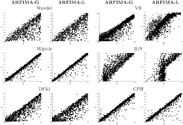
Figure 3: Estimates of $H$ for walks derived from ARFIMA-G(1,d,1) and ARFIMA-L(1,d,1) with the Wavelet method and Variable Bandwidth estimator $\mathrm{VB}$. Estimates of $d$ for ARFIMA-G(1,d,1) and ARFIMA-L(1,d,1) for the Whittle estimator, $R/S$, DFA1 and GPH. The solid line indicates the true self-similarity parameter $H$.

4.2 Trends

Another important test is to see how the presence of trends affects the various estimators. Here we consider three cases: 1) a linear trend superimposed by realisations of fGn, oLn, ARFIMA-G and ARFIMA-L; and 2) a linear trend only in the second half of the time series superimposed by realisations of fGn, oLn, ARFIMA-G and ARFIMA-L; 3) a linear trend in the variance. Cases 2 and 3 are motivated by climate change where the time series may (case 2) or may not (case 1) include the pre-industrial era, and where climate change also influences the frequency and strength of fluctuations (e.g. storms; case 3). Based on the evidence gathered so far, it is reasonable to expect this can lead to bias any long-range dependence estimate.

For cases 1 and 2, we assume the magnitude of the linear trend to be 1. The empirical tests reveal that the GPH estimator is slightly biased for fGn, ARFIMA-G and ARFIMA-L and has a relatively large negative bias for oLn (Figs. 5). DFA is least biased for fGn data but has considerable bias for oLn, ARFIMA-G and ARFIMA-L (Figs. 5) generated data. Both ARFIMA-G and ARFIMA-L estimators have a large number of outliers. Both $R/S$ and $\mathrm{VB}$ show qualitatively similar behaviour compared to GPH (not shown). Our results are qualitatively consistent with the study by Hu et al. (2001).

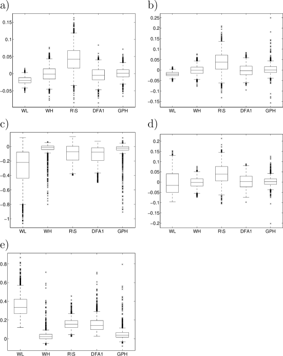
Figure 4: Box plots of the difference between the nominal parameter value and the empirical parameter estimate: a) uncorrelated Gaussian white noise, b) AR(1) and c) ARFIMA-G(1,0,1), d) AR(1) process with linear trend in variance and e) Markovian SDE with CAM noise. On each box the central mark is the median, the edges of the boxes are the 25th and 75th percentiles, the whiskers extend to the most extreme data points not considered to be outliers and outliers are marked individually.

Now we examine how the estimators handle a trend in the variance (case 3). For this purpose we use an AR(1) model with increasing variance:

$$x_{t+1}=F+\alpha x_{t}+\sigma(1+\frac{t}{10000})\zeta_{t}.$$ (12)

Here, again, we generate 1000 realisations by sampling values for F from a uniform distribution $U(0,2)$, using $\alpha\in U(-0.5,0.5)$, and $\sigma\in U(0,1)$. For this case DFA is the least biased and GPH and $R/S$ show considerable bias while the $\mathrm{VB}$ estimators have a huge bias, although, their estimates are very narrow (Fig. 4e).

4.3 CAM noise

Both LFSM and ARFIMA are additive noise models. In previous studies it has been shown that multiplicative noise is important in natural systems (e.g. Majda et al. 2009, Steinbrecher and Weyssow 2004). This raises the question of what the effect of multiplicative noise would be on long-range dependence estimators. To investigate, we use data generated from a process which has a so called Correlated Additive and Multiplicative (CAM) noise term. An example is the normal form for reduced climate models (Majda et al. 2009), which is given by the following Stochastic Differential Equation (SDE):

$$dx=(F+ax+bx^{2}-cx^{3})dt+\sigma(L+Ix)dW.$$ (13)

As shown in Majda et al. (2009), the PDF of Eq. (13) exhibits a power-law decay over a particular range, although its tail ultimately decays exponentially. We generate 1000 realisations by sampling random values for the SDE parameters from an uniform distribution while complying with the parameter relations as described in Majda et al. (2009).

The GPH estimator is slightly biased towards positive values while DFA and $R/S$ have larger biases. Observe that the Wavelet estimator (as well as both $\mathrm{VB}$ estimators (not shown)) estimate self-similar behaviour (Fig. 4f). While the PDF of Eq. (13) decays in a power-law like way over a given range it is not self-similar because its ultimate decay is exponential (Majda et al. 2009). This makes the estimates obtained by the wavelet and $\mathrm{VB}$ estimators questionable. Furthermore, $R/S$, DFA, GPH and the Whittle estimator again show an uncomfortably large number of outliers, again suggesting that the estimators may not be very reliable for this case, or that the signal is not characterised simply by $H$ and $d$. We note that Kantelhardt et al. (2002) have studied the performance of more general multifractal DFA methods which were found to extract the full range of scaling exponents in a particular multifractal test case.

5 Natural Time Series Examples

Now we return to the two natural time series from Section 2, and analyse their self-similarity and LRD characteristics. We have shown above that the two time series are non-Gaussian; are they also long-range dependent or self-similar?

Applying the various estimation methods to the Faraday-Vernadsky temperature time series gives evidence for long-range dependence but with a wide variety of values: Whittle $d=0.24$, GPH $d=0.28$, DFA2 $d=0.43$, $R/S$ $d=0.33$, Wavelet $H=0.53$, $\mathrm{VB}_{w}$ $H=0.92$ and $\mathrm{VB}_{\delta}$ $H=0.96$. While the three LRD estimators all provide evidence for long range dependence, they provide a rather large range of values of the LRD parameter, $d$. However, all of the estimates are between 0 and 0.5, suggesting a long-range dependent but stationary process. The $H$ estimates are larger than the $d$ estimates; this might suggest self-similarity with $\alpha\approx 1.5$.

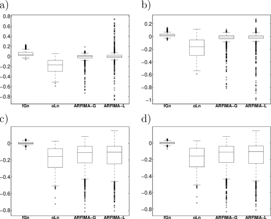
Figure 5: Box plots of the difference between the nominal parameter value and the empirical parameter estimate a) GPH estimator for noise plus linear trend, b) GPH estimator for noise plus linear trend in second half of time series, c) DFA2 estimator for noise plus linear trend and d) DFA2 estimator for noise plus linear trend in second half of time series. On each box the central mark is the median, the edges of the boxes are the 25th and 75th percentiles, the whiskers extend to the most extreme data points not considered to be outliers and outliers are marked individually.

There is also evidence for long-range dependence in the AE index, again with a wide variety of estimates from the various estimators: Whittle $d=0.28$, GPH $d=0.72$, DFA2 $d=0.66$, $R/S$ $d=0.4$, Wavelet $H=0.94$, $\mathrm{VB}_{w}$ $H=0.97$ and $\mathrm{VB}_{\delta}$ $H=0.99$. The estimates from GPH and DFA2 are larger than 0.5, suggesting a non-stationary time series, while the Whittle and $R/S$ estimates suggests a stationary long-range dependent time series. Again the $H$ estimates are larger than the $d$ estimates, providing some evidence for self-similarity. Other evidence has been presented that AE may not be a simple fractal (Consolini et al. 1996); recently work has focused on high-frequency non-stationary and lower-frequency $1/f$ properties (Rypdal and Rypdal 2010).

While all LRD estimators agree that there is evidence for LRD in these two time series they provide a rather large range of possible values, illustrating the problem of statistically robust LRD estimation in practice and the need for further investigation of the performance of statistical indicators in the presence of departures from fractality, including possible multifractality.

6 Conclusions

There are two contributions to self-similarity: (i) long-range dependence and (ii) non-Gaussian jumps. This is not always appreciated in the various communities with interests in detecting self-similarity and long-range dependence. We have shown that empirical estimators of long-range dependence are at best biased for fractional Gaussian noise, but at worst not robust for processes which deviate from this idealised model. We have also shown that the empirical estimators are not very robust in the presence of trends and multiplicative noise.

Our results have several important implications for the modelling of natural time series. In our view the ARFIMA model is a much better paradigmatic model of natural time series than fGn since it allows one to explicitly model short-range and long-range behaviour while also allowing for non-Gaussian increments.

Finally, there is a need for estimation procedures which can deal with multiplicative noise and trends in the variance. Such effects introduce sizeable biases and estimation uncertainty. As such, all estimations of LRD have to be taken with precaution. While it is true that all of the estimators we tested perform reasonably well for fractional Gaussian noise, once a time series is non-Gaussian or is non-stationary (in trend or volatility) the estimators can be problematic.

- [1] Abry, P. and D. Veitch, 1998: Wavelet Analysis of Long-Range-Dependent Traffic. IEEE Trans. Inform. Theo., 44, 2-15.
- [2] Bardet, J.-M., E. Moulines and P. Soulier: Recent advances on the semi-parametric estimation of the long-range dependence coefficient. ESAIM Proc., 5, 29-41, Soc. Math. Appl. Indust., 1998.
- [3] Bashan, A., R. Bartsch, J. W. Kantelhardt and S. Havlin: Comparison of detrending methods for fluxtuation analysis, Physica A, 387, 5080-5090, 2008.
- [4] Beran, J., Statistics for Long-Memory Processes. Chapman Hall, 1994.
- [5] Bogachev, M., J. Eichner and A. Bunde: On the occurrence of extreme events in long-term correlated and multifractal data sets. Pure Appl. Geophysics, 165, 1195-1207, 2008.
- [6] Box, G. and G. Jenkins, Time series analysis: forecasting and control, Holden Day, San Francisco, 1970
- [7] Bunde, A., J. Eichner, J. Kantelhardt and S. Havlin: Long-term memory: A natural mechanism for the clustering of extreme events and anomalous residual times in climate records. Phys. Rev. Lett., 94, 2005, doi:10.1103/PhysRevLett.94.048701
- [8] Chen, Z., P. Ch. Ivanov, K. Hu and H. E. Stanley: Effect of nonstationarities on detrended fluctuation analysis, Phys. Rev. E., 65, 041107, 2002.
- [9] Consolini, G., M. F. Marcucci and M. Candidi: Multifractal structure of Auroral Electrojet index data. Phys. Rev. Lett., 76, 4082-4085.
- [10] Davis, T. and M. Sugiura: Auroral Electrojet Activity Index AE and its universal time variations. J. Geophys. Res., 71, 785-801, 1966
- [11] Einstein, A.: Über die von der molekularkinetischen Theorie der Wärme geförderte Bewegung von in ruhenden Flüssigkeiten suspendierten Teilchen. Annalen der Physik, 17, 549-560, 1905.
- [12] Embrechts, P. and M. Maejima: Selfsimilar Processes. Princeton Series in Applied Mathematics. Princeton University Press. 111p, 2002.
- [13] Escorcia-Garcia, J., R. Cruz-Silva and V. Agarwal: Self-affinity study of nano-structured porous silicon-crystalline silicon interfaces. Applied Surface Science, 256, 645-649, 2009.
- [14] Franzke, C.: Long-range dependence and climate noise characteristics of Antarctic temperature data. J. Climate, 23, 2010, doi: 10.1175/2010JCLI3654.1.
- [15] Geweke, J. and S. Porter-Hudak, The estimation and application of long-memory time series models, Journal of Time Series Analysis, 4:221-238, 1983
- [16] Ghil, M., et al.: Extreme Events: Dynamics, Statistics and Prediction. Nonlin. Processes Geophys., 18, 295-350, 2011. doi:10.5194/npg-18-295-2011
- [17] Kantelhardt, J., S. A. Zschiegner, E. Koscielny-Bunde, S. Havlin, A. Bunde and H. E. Stanley: Multifractal detrended fluctuation analysis of nonstationary time series. Physica A, 316, 87-114, 2002.
- [18] Kropp, J. and H.-J. Schellnhuber: In Extremis: Disruptive Events and Trends in Climate and Hydrology, Springer, 320pp, 2010.
- [19] Hasselmann, K.: Stochastic climate models. Part I: Theory. Tellus, 6, 473-484, 1976.
- [20] Hu, K., P. Ch. Ivanov, Z. Chen, P. Cadrena and H. E. Stanley: Effect of nonstationarities on detrended fluctuation analysis, Phys. Rev. E., 64, 011114, 2001.
- [21] Hurst, H., Long-Term Storage capacity of reservoirs, Trans. Am. Resour. Res., 14(3), 509-516, 1951
- [22] Hurst, H., R. Black and Y. Simaika, Long-Term Storage: An Experimental Study, Constable, London, 1965
- [23] Hurvich, C., R. Deo and J. Brodsky, The mean squared error of Geweke and Porter-Hudak’s estimator of the memory parameter of a long memory time series, Journal of Time Series Analysis, 19:19-46, 2001
- [24] Hurvich, C., E. Moulines and P. Soulier, The FEXP estimator for potentially non-stationary linear time series, Stochastic Process. Appl., 97:307-340, 2002
- [25] Hurvich, C., E. Moulines and P. Soulier, Estimating long memory in volatility, Econometrica, 73:1283-1328, 2005
- [26] Huybers, P and W. Curry: Links between annual, Milankovitch and continuum temperature variability. Nature, 441, 329-332, 2006. doi:10.1038/nature04745
- [27] Lenton, T. M., V. N. Livina, V. Dakos, E. H. van Nes and M. Scheffer, 2011: Early warning of climate tipping points from critical slowing down: comparing methods to improve robustness. Phil. Trans. R. Soc. A, this issue.
- [28] Livina, V. N. and T. M. Lenton: A modified method for detecting incipient bifurcations in a dynamical system. Geophys. Res. Lett., 34, L03712, doi:10.1029/2006GL028672, 2007
- [29] Lorenz, E. N.: Deterministic Nonperiodic Flow. J. Atmos. Sci., 20, 130-141, 1963
- [30] Majda, A., C. Franzke and D. Crommelin: Normal forms for reduced stochastic climate models. Proc. Nat. Acad. Sci. USA, 106, doi:10.1073/pnas.0900173106, 2009.
- [31] Mailier, P., D. Stephenson and C. Ferro, Serial Clustering of Extratropical Storms. Mon. Wea. Rev., 134, 2224-2240, 2006
- [32] Mandelbrot, B. and J. Wallis: Noah, Joseph, and Operational Hydrology. Water Resources Res., 4, 909-918, 1968.
- [33] Mandelbrot, B.: Gaussian Self-Afinity and Fractals, Springer, New York, 2001.
- [34] Maraun, D., H. W. Rust and J. Timmer: Tempting long-memory - on the interpretation of DFA results. Nonlinear Proc. Geophys., 11, 495-503, 2004.
- [35] Mercik, S., K. Weron, K. Burnecki and A. Weron: Enigma of self-similarity of fractional Levy stable motions. Acta Phys. Pol. B. 34, 3773, 2003.
- [36] Ogurtsov, M. G., New evidence for long-term persistence in the sun’s activity, Solar Physics, 220, 93-105, 2004.
- [37] Peng, C., S. Buldyrev, S. Havlin, M. Simons, H. Stanley and A. Goldberger, Mosaic organization of DNA nucleotides, Phys. Rev. E, 49:1685-1689, 1994
- [38] Price, C. P. and D. E. Newman: Using the R/S statistic to analyze AE data, Journal of Atmospheric and Solar-Terrestrial Physics, 63, 1387-1397,2001.
- [39] Robinson, P. M.: Log-periodogram regression of time series with long-range dependence. Ann. Statist., 23, 1048-1072, 1995a.
- [40] Robinson, P. M.: Gaussian semiparametric estimation of long range dependence. Ann. Statis., 23, 1630-1661, 1995b.
- [41] Rust, H. W., O. Mestre and V. K. C. Venema: Fewer jumps, less memory: Homogenized temperature records and long memory. J. Geophys. Res., 113, D19110, 2008, doi: 10.1029/2008JD009919
- [42] Rypdal, M. and K. Rypdal: Stochastic modeling of the AE index and its relation to fluctuations in of the IMF on time scales shorter than substorm duration. J. Geophys. Res., 115, A11216, 2010. doi:10.1029/2010JA015463
- [43] Samorodnitsky, G. and M. Taqqu: Stable non-Gaussian Random Processes. Chapman & Hall, 632p., 1994
- [44] Scipioni, A., P. Rischette, G. Bonhomme, and P. Devynck, Characterization of self-similarity properties of turbulence in magnetized plasmas, Phys. Plasmas, 15, 112303, doi:10.1063/1.3006075, 2008.
- [45] Shimotsu, K. and P. C. B. Phillips, 2005: Exact Local Whittle Estimation of Fractional Integration. Annals of Statistics, 33, 1890-1933.
- [46] Shimotsu, K. and P. C. B. Phillips, 2006: Local Whittle Estimation of Fractional Integration and some of its variants. J. Econometrics, 130, 209-233.
- [47] Sieber, J. and M. T. Thompson, 2011: Nonlinear softening as a predictive precursor to climate tipping. Phil. Trans. R. Soc. A., this issue.
- [48] Schmittbuhl, J., Vilotte, J.-P. and S. Roux: Reliability of self-affine measurements. Phys. Rev. E, 51, 131-147, 1995.
- [49] Steinbrecher, G. & B. Weyssow, 2004: Generalized randomly amplified linear system driven by Gaussian noises: Extreme heavy tail and algebraic correlation decay in plasma turbulence. Phys. Rev. Lett., 92, doi: 10.1103/PhysRevLett.92.125003
- [50] Stoev, S. and M. Taqqu, Simulation methods for linear fractional stable motion and FARIMA using the Fast Fourier Transform, Fractals, 12:95-121, 2004
- [51] Stoev, S. and M. Taqqu, 2005: Asymptotic self-similarity and wavelet estimation for long-range dependent fractional autoregressive integrated moving average time series with stable innovations, J. Time Series Ana., 26, 211-249.
- [52] Stoev, S., M. S. Taqqu, C. Park and J. S. Marron: On the wavelet spectrum diagnostic for Hurst parameter estimation in the analysis of Internet traffic. Computer Networks, 48, 423-445, 2005.
- [53] Taqqu, M.: Fractional Brownian motion and long-range dependence. In Doukhan et al., Eds. 2003, Theory and Applications of Long-range dependence. Birkhäuser. pp. 5-42.
- [54] Taqqu, M. , V. Teverosky and W. Willinger: Estimators for long-range dependence: an empirical study. Fractals, 3, 785-798, 1995.
- [55] Tuck, A. F. and S. J. Hovde: Fractal behavior of ozone, wind and temperature in the lower stratosphere. Geophys. Res. Lett., 26, 1271-1274, 1999. doi:10.1029/1999GL900233
- [56] Turner, J., et al: The SCAR READER Project: Toward a high-quality database of mean Antarctic Meteorological Observations. J. Climate, 17, 2890-2898, 2004.
- [57] Vyushin, D and P. Kushner: Power-law and long-memory characteristics of the atmospheric general circulation. J. Climate, 22, 2890-2904, 2009.
- [58] Watkins, N.: Scaling in the space climatology of the auroral indices: is SOC the only possible description? Nonlin. Processes Geophys., 9, 389-397, 2002.