Order Statistics Based List Decoding Techniques for Linear Binary Block Codes

Abstract

The order statistics based list decoding techniques for linear binary block codes of small to medium block length are investigated. The construction of the list of the test error patterns is considered. The original order statistics decoding is generalized by assuming segmentation of the most reliable independent positions of the received bits. The segmentation is shown to overcome several drawbacks of the original order statistics decoding. The complexity of the order statistics based decoding is further reduced by assuming a partial ordering of the received bits in order to avoid the complex Gauss elimination. The probability of the test error patterns in the decoding list is derived. The bit error rate performance and the decoding complexity trade-off of the proposed decoding algorithms is studied by computer simulations. Numerical examples show that, in some cases, the proposed decoding schemes are superior to the original order statistics decoding in terms of both the bit error rate performance as well as the decoding complexity.

I Introduction

A major difficulty in employing forward error correction (FEC) coding is the implementation complexity especially of the decoding at the receiver and the associated decoding latency for long codewords. Correspondingly, the FEC coding is often designed to trade-off the bit error rate (BER) with the decoding complexity and latency. Many universal decoding algorithms have been proposed for the decoding linear binary block codes [1]. The decoding algorithms in [3]–[11] are based on the testing and re-encoding of the information bits as initially considered by Dorsch in [2]. In particular, a list of the likely transmitted codewords is generated using the reliabilities of the received bits, and then, the most likely codeword is selected from this list. The list of the likely transmitted codewords can be constructed from a set of the test error patterns. The test error patterns can be predefined as in [3] and [4] and in this paper, predefined and optimized for the channel statistics as in [5], or defined adaptively for a particular received sequence as suggested in [6]. The complexity of the list decoding can be further reduced by the skipping and stopping rules as shown, for example, in [3] and [4].

Among numerous variants of the list decoding techniques, the order statistics decoding (OSD) is well-known [3], [4]. The structural properties of the FEC code are utilized to reduce the OSD complexity in [7]. The achievable coding gain of the OSD is improved by considering the multiple information sets in [8]. The decoding proposed in [9] exploits randomly generated biases to present the decoder with the multiple received soft-decision values. The sort and match decoding of [10] divides the received sequence into two disjoint segments. The list decoding is then performed for each of the two segments independently, and the two lists are combined using the sort and match algorithm to decide on the most likely transmitted codeword. The box and match decoding strategy is developed in [11]. An alternative approach to the soft-decision decoding of linear binary block codes relies on the sphere decoding techniques [12, 13]. For example, the input sphere decoder (ISD) discussed in this paper can be considered to be a trivial sphere decoding algorithm.

In this paper, we investigate the OSD-based decoding strategies for linear binary block codes. Our aim is to obtain low-complexity decoding schemes that provide sufficiently large or valuable coding gains, and most importantly, that are well-suited for implementation in communication systems with limited hardware resources, e.g., at nodes of the wireless sensor network. We modify the original OSD by considering the disjoint segments of the most reliable independent positions (MRIPs). The segmentation of the MRIPs creates flexibility that can be exploited to fine tune a trade-off between the BER performance and the decoding complexity. Thus, the original OSD can be considered to be a special case of the segmentation-based OSD having only one segment corresponding to the MRIPs. Since the complexity of obtaining a row echelon form of the generator matrix for every received codeword represents a significant part of the overall decoding complexity, we examine a partial-order statistics decoding (POSD) when only the systematic part of the received codeword is ordered.

This paper is organized as follows. System model is described in Section II. Construction of the list of test error patterns is investigated in Section III. The list decoding algorithms are developed in Section IV. The performance analysis is considered in Section V. Numerical examples to compare the BER performance and the decoding complexity of the proposed decoding schemes are presented in Section VI. Finally, conclusions are given in Section VII.

II System Model

Consider transmission of codewords of a linear binary block code $\mathcal{C}$ over an additive white Gaussian noise (AWGN) channel with Rayleigh fading. The code $\mathcal{C}$, denoted as $(N,K,{d_{\mathrm{min}}})$, has block length $N$, dimension $K$, and the minimum Hamming distance between any two codewords ${d_{\mathrm{min}}}$. Binary codewords $\mathbf{c}\in\mathbb{Z}_{2}^{N}$ where $\mathbb{Z}_{2}=\{0,1\}$ are generated from a vector of information bits $\mathbf{u}\in\mathbb{Z}_{2}^{K}$ using the generator matrix $\mathbf{G}\in\mathbb{Z}_{2}^{K\times N}$, i.e., $\mathbf{c}=\mathbf{u}\mathbf{G}$, and all binary operations are considered over a Galois field $\mathrm{GF}(2)$. If the code $\mathcal{C}$ is systematic, the generator matrix has the form, $\mathbf{G}=[\mathbf{I}\ \mathbf{P}]$, where $\mathbf{I}$ is the $K\times K$ identity matrix, and $\mathbf{P}\in\mathbb{Z}_{2}^{K\times(N-K)}$ is the matrix of parity checks. The codeword $\mathbf{c}$ is mapped to a binary phase shift keying (BPSK) sequence $\mathbf{x}\in\{+1,-1\}^{N}$ before transmission using a mapping, $x_{i}={\mathcal{M}}\left(c_{i}\right)=(-1)^{c_{i}}$, for $i=1,2,\cdots,N$. Assuming bits $u_{i}$ and $u_{j}$, the mapping $\mathcal{M}$ has the property,

$${\mathcal{M}}\left(u_{i}\oplus u_{j}\right)={\mathcal{M}}\left(u_{i}\right){\mathcal{M}}\left(u_{j}\right)$$ (1)

where $\oplus$ denotes the modulo $2$ addition. The encoded bit $c_{i}$ can be recovered from the symbol $x_{i}$ using the inverse mapping, $c_{i}={\mathcal{M}^{-1}}\left(x_{i}\right)=(1-x_{i})/2$. For brevity, we also use the notation, $\mathbf{x}={\mathcal{M}}\left(\mathbf{c}\right)$ and $\mathbf{c}={\mathcal{M}^{-1}}\left(\mathbf{x}\right)$, to denote the component-wise modulation mapping and de-mapping, respectively. The code $\mathcal{C}$ is assumed to have equally probable values of the encoded bits, i.e., the probability, $\mathrm{Pr}\!\left\{c_{i}=0\right\}=\mathrm{Pr}\!\left\{c_{i}=1\right\}=1/2$, for $i=1,2,\cdots,N$. Consequently, all the codewords are transmitted with the equal probability, i.e., $\mathrm{Pr}\!\left\{\mathbf{c}\right\}=2^{-K}$ for $\forall\mathbf{c}\in\mathcal{C}$.

The signal at the output of the matched filter at the receiver can be written as,

$$y_{i}=h_{i}x_{i}+w_{i}$$

where the frequency non-selective channel fading coefficients $h_{i}$ as well as the AWGN samples $w_{i}$ are mutually uncorrelated zero-mean circularly symmetric complex Gaussian random variables. The variance of $h_{i}$ is unity, i.e., $\mathrm{E}\!\left[|h_{i}|^{2}\right]=1$ where $\mathrm{E}\!\left[\cdot\right]$ is expectation, and $|\cdot|$ denotes the absolute value. The samples $w_{i}$ have the variance, $\mathrm{E}\!\left[|w_{i}|^{2}\right]=(R\gamma_{c})^{-1}$, where $R=K/N$ is the coding rate of $\mathcal{C}$, and $\gamma_{c}$ is the signal-to-noise ratio (SNR) per transmitted encoded binary symbol. The covariance, $\mathrm{E}\!\left[h_{i}h_{j}^{\ast}\right]=0$ for $i\neq j$, where $(\cdot)^{\ast}$ denotes the complex conjugate, corresponds to the case of a fast fading channel with ideal interleaving and deinterleaving. For a slowly block-fading channel, the covariance, $\mathrm{E}\!\left[h_{i}h_{j}^{\ast}\right]=1$ for $\forall i,j=1,2,\cdots,N$, and the fading coefficients are uncorrelated between transmissions of adjacent codewords.

In general, denote as $f(\cdot)$ the probability density function (PDF) of a random variable. The reliability $r_{i}$ of the received signal $y_{i}$ corresponds to a ratio of the conditional PDFs of $y_{i}$ [14], i.e.,

$$\frac{f(y_{i}|x_{i}=+1,h_{i})}{f(y_{i}|x_{i}=-1,h_{i})}\propto\mathrm{Re}\!\left\{h_{i}^{\ast}y_{i}\right\}=r_{i}$$

since the PDF $f(y_{i}|x_{i},h_{i})$ is conditionally Gaussian. Thus, the reliability $r_{i}$ can be written as,

$$r_{i}=\mathrm{Re}\!\left\{h_{i}\right\}\mathrm{Re}\!\left\{y_{i}\right\}+\mathrm{Im}\!\left\{h_{i}\right\}\mathrm{Im}\!\left\{y_{i}\right\}=|h_{i}|^{2}x_{i}+|h_{i}|w_{i}.$$

The bit-by-bit quantized (i.e., hard) decisions are then defined as,

$$\hat{c}_{i}={\mathcal{M}^{-1}}\left(\mathrm{sign}\!\left(r_{i}\right)\right)$$

where $\mathrm{sign}\!\left(\cdot\right)$ denotes the sign of a real number.

More importantly, even though the primary metric of our interest is the BER performance of the code $\mathcal{C}$, it is mathematically more convenient to obtain and analyze the list decoding algorithms assuming the probability of codeword error. Thus, we assume that the list decoding with a given decoding complexity obtained for the probability of codeword error will also have a good BER performance. The maximum likelihood (ML) decoder minimizing the probability of codeword error provides the decision $\hat{\mathbf{c}}_{\mathrm{ML}}$ on the most likely transmitted codeword, i.e.,

$$\hat{\mathbf{c}}_{\mathrm{ML}} = \mathop{\rm argmin}_{\mathbf{c}\in\mathcal{C}:\ \mathbf{x}={\mathcal{M}}\left(\mathbf{c}\right)}\left\|\mathbf{y}-\mathbf{h}\odot\mathbf{x}\right\|^{2}$$ (2)

$$= \mathop{\rm argmax}_{\mathbf{c}\in\mathcal{C}}\sum_{i=1}^{N}\mathrm{Re}\!\left\{y_{i}h_{i}^{\ast}x_{i}^{\ast}\right\}\overset{\mbox{\footnotesize BPSK}}{=}\mathop{\rm argmax}_{\mathbf{c}\in\mathcal{C}:\ \mathbf{x}={\mathcal{M}}\left(\mathbf{c}\right)}\ \mathbf{r}\cdot\mathbf{x}$$

where $\mathbf{y}$, $\mathbf{h}$, $\mathbf{x}$, and $\mathbf{r}$ denote the $N$-dimensional row vectors of the received signals $y_{i}$, the channel coefficients $h_{i}$, the transmitted symbols $x_{i}$, and the reliabilities $r_{i}$ within one codeword, respectively, $\left\|\cdot\right\|$ is the Euclidean norm of a vector, $\odot$ is the component-wise (Hadamard) product of vectors, and the binary operator $\cdot$ is used to denote the dot-product of vectors. The codewords $\mathbf{c}\in\mathcal{C}$ used in (2) to find the maximum or the minimum value of the ML metric are often referred to as the test codewords. In the following subsection, we investigate the soft-decision decoding algorithms with low implementation complexity to replace the computationally demanding ML decoding (2).

II-A List Decoding

We investigate the list-based decoding algorithms. For simplicity, we assume binary block codes that are linear and systematic [15]. We note that whereas the extension of the list-based decoding algorithms to non-systematic codes is straightforward, the list based decoding of non-linear codes is complicated by the fact that the list of the test codewords is, in general, dependent on the received sequence. The decoding (time) complexity $O$ of the list decoding algorithms can be measured as the list size given by the number of the test codewords that are examined in the decoding process. Thus, the ML decoding (2) has the complexity, $O_{\mathrm{ML}}=2^{K}$, which is prohibitive for larger values of $K$. Among the practical list-based decoding algorithms with the acceptable decoding complexity, we investigate the order statistics decoding (OSD) [3] based list decoding algorithms for soft-decision decoding of linear binary block codes.

The OSD decoding resumes by reordering the received sequence of reliabilities as,

$$|\tilde{r}_{1}^{\prime}|\geq|\tilde{r}_{2}^{\prime}|\geq\cdots|\tilde{r}_{N}^{\prime}|$$ (3)

where the tilde is used to denote the ordering. This ordering of the reliabilities defines a permutation, $\lambda^{\prime}$, i.e.,

$$\tilde{\mathbf{r}}^{\prime}=\lambda^{\prime}\!\left[\mathbf{r}\right]=(\tilde{r}_{1}^{\prime},\cdots,\tilde{r}_{N}^{\prime}).$$

The permutation $\lambda^{\prime}$ corresponds to the generator matrix $\tilde{\mathbf{G}}^{\prime}=\lambda^{\prime}\!\left[\mathbf{G}\right]$ having the reordered columns. In order to obtain the most reliable independent positions (MRIPs) for the first $K$ bits in the codeword, additional swapping of the columns of $\tilde{\mathbf{G}}^{\prime}$ may have to be used which corresponds to the permutation $\lambda^{\prime\prime}$, and the generator matrix $\tilde{\mathbf{G}}^{\prime\prime}=\lambda^{\prime\prime}\!\left[\tilde{\mathbf{G}}^{\prime}\right]$. The matrix $\tilde{\mathbf{G}}^{\prime\prime}$ can be manipulated into a row (or a reduced row) echelon form using the Gauss (or the Gauss-Jordan) elimination. To simplify the notation, let $\tilde{\mathbf{r}}$ and $\tilde{\mathbf{G}}$ denote the reordered sequence of the reliabilities $\mathbf{r}$ and the reordered generator matrix $\tilde{\mathbf{G}}$ in a row (or a reduced row) echelon form, respectively, after employing the permutations $\lambda^{\prime}$ and $\lambda^{\prime\prime}$, to decode the received sequence $\mathbf{y}$. Thus, for $i\geq j$, the reordered sequence $\tilde{\mathbf{r}}$ has elements, $|\tilde{r}_{i}|\geq|\tilde{r}_{j}|$, for $i,j=1,\cdots,K$, and for $i,j=K+1,\cdots,N$.

The complexity of the ML decoding (2) of the received sequence $\mathbf{y}$ can be reduced by assuming a list of the $L$ test codewords, so that $L\ll 2^{K}$. Denote such a list of the test codewords of cardinality $L$ generated by the matrix $\tilde{\mathbf{G}}$ as, $\mathcal{E}_{L}=\{\mathbf{e}_{0},\mathbf{e}_{2},\cdots,\mathbf{e}_{L_{-}1}\}$, and let $\mathbf{e}_{0}=\mathbf{0}$ be the all-zero codeword. Then, the list decoding of $\mathbf{y}$ is defined as,

$$\hat{\mathbf{c}}=\mathop{\rm argmax}_{\mathbf{e}\in\mathcal{E}_{L}:\ \mathbf{x}={\mathcal{M}}\left(\hat{\mathbf{c}}_{0}\oplus\mathbf{e}\right)}\tilde{\mathbf{r}}\cdot\mathbf{x}$$ (4)

where the systematic part of the codeword $\hat{\mathbf{c}}_{0}$ is given by the hard-decision decoded bits at the MRIPs. The decoding step to obtain the decision $\hat{\mathbf{c}}_{0}$ is referred to as the $0$-th order OSD reprocessing in [3]. In addition, due to linearity of $\mathcal{C}$, we have that $(\mathbf{c}_{0}\oplus\mathbf{e})\in\mathcal{C}$, and thus, the test codewords $\mathbf{e}\in\mathcal{E}_{L}$ can be also referred to as the test error patterns in the decoding (4). Using the property (1), we can rewrite the decoding (4) as,

$$\hat{\mathbf{c}}=\mathop{\rm argmax}_{\mathbf{e}\in\mathcal{E}_{L}}\ \tilde{\mathbf{r}}\cdot\hat{\mathbf{x}}_{0}\cdot{\mathcal{M}}\left(\mathbf{e}\right)=\mathop{\rm argmax}_{\mathbf{e}\in\mathcal{E}_{L}}\ \tilde{\mathbf{r}}_{0}\cdot{\mathcal{M}}\left(\mathbf{e}\right)$$ (5)

where we denoted $\hat{\mathbf{x}}_{0}={\mathcal{M}}\left(\hat{\mathbf{c}}_{0}\right)$ and $\tilde{\mathbf{r}}_{0}=\tilde{\mathbf{r}}\odot\hat{\mathbf{x}}_{0}$. The system model employing the list decoding (5) is illustrated in Fig. 1. More importantly, as indicated in Fig. 1, the system model can be represented as an equivalent channel with the binary vector input $\mathbf{c}$ and the vector soft-output $\tilde{\mathbf{r}}_{0}$.

III List Selection

The selection of the test error patterns $\mathbf{e}$ to the list $\mathcal{E}_{L}$ as well as the list size $L$ have a dominant effect upon the probability of incorrect codeword decision by the list decoding. Denote such probability of codeword error as $\mathrm{P_{e}}$, and let $\mathbf{c}_{\mathrm{Tx}}$ be the transmitted codeword. In [12], the probability $\mathrm{P_{e}}$ is expanded as,

$$\mathrm{P_{e}} = \mathrm{Pr}\!\left\{\hat{\mathbf{c}}\neq\mathbf{c}_{\mathrm{Tx}}|\hat{\mathbf{c}}_{\mathrm{ML}}\neq\mathbf{c}_{\mathrm{Tx}}\right\}\mathrm{Pr}\!\left\{\hat{\mathbf{c}}_{\mathrm{ML}}\neq\mathbf{c}_{\mathrm{Tx}}\right\}$$

$$+\mathrm{Pr}\!\left\{\hat{\mathbf{c}}\neq\mathbf{c}_{\mathrm{Tx}}|\hat{\mathbf{c}}_{\mathrm{ML}}=\mathbf{c}_{\mathrm{Tx}}\right\}\mathrm{Pr}\!\left\{\hat{\mathbf{c}}_{\mathrm{ML}}=\mathbf{c}_{\mathrm{Tx}}\right\}$$

where the decision $\hat{\mathbf{c}}$ is obtained by the decoding (5), and the condition, $\hat{\mathbf{c}}_{\mathrm{ML}}\neq\mathbf{c}_{\mathrm{Tx}}$, is true provided that the vectors $\hat{\mathbf{c}}_{\mathrm{ML}}$ and $\mathbf{c}_{\mathrm{Tx}}$ differ in at least one component, i.e., $\hat{\mathbf{c}}_{\mathrm{ML}}=\mathbf{c}_{\mathrm{Tx}}$ if and only if all the components of the vectors are equal. Since, for any list $\mathcal{E}_{L}$, the probability, $\mathrm{Pr}\!\left\{\hat{\mathbf{c}}\neq\mathbf{c}_{\mathrm{Tx}}|\hat{\mathbf{c}}_{\mathrm{ML}}\neq\mathbf{c}_{\mathrm{Tx}}\right\}=1$, and usually, the probability, $\mathrm{Pr}\!\left\{\hat{\mathbf{c}}_{\mathrm{ML}}=\mathbf{c}_{\mathrm{Tx}}\right\}$ is close to $1$, $\mathrm{P_{e}}$ can be tightly upper-bounded as,

$$\mathrm{P_{e}}\leq\mathrm{Pr}\!\left\{\hat{\mathbf{c}}_{\mathrm{ML}}\neq\mathbf{c}_{\mathrm{Tx}}\right\}+\mathrm{Pr}\!\left\{\hat{\mathbf{c}}\neq\mathbf{c}_{\mathrm{Tx}}|\hat{\mathbf{c}}_{\mathrm{ML}}=\mathbf{c}_{\mathrm{Tx}}\right\}.$$ (6)

The first term on the right hand side of (6) is the codeword error probability of the ML decoding, and the second term is the conditional codeword error probability of the list decoding. The probability, $\mathrm{Pr}\!\left\{\hat{\mathbf{c}}\neq\mathbf{c}_{\mathrm{Tx}}|\hat{\mathbf{c}}_{\mathrm{ML}}=\mathbf{c}_{\mathrm{Tx}}\right\}$, is decreasing with the list size. In the limit of the maximum list size when the list decoding becomes the ML decoding, the bound (6) becomes, $\mathrm{P_{e}}=\mathrm{Pr}\!\left\{\hat{\mathbf{c}}_{\mathrm{ML}}\neq\mathbf{c}_{\mathrm{Tx}}\right\}$. The bound (6) is particularly useful to analyze the performance of the list decoding (5). However, in order to construct the list of the test error patterns, we consider the following expansion of the probability $\mathrm{P_{e}}$, i.e.,

$$\mathrm{P_{e}} = \mathrm{Pr}\!\left\{\hat{\mathbf{c}}\neq\mathbf{c}_{\mathrm{Tx}}|(\mathbf{c}_{\mathrm{Tx}}\oplus\hat{\mathbf{c}}_{0})\in\mathcal{E}_{L}\right\}\mathrm{Pr}\!\left\{(\mathbf{c}_{\mathrm{Tx}}\oplus\hat{\mathbf{c}}_{0})\in\mathcal{E}_{L}\right\}$$

$$+\mathrm{Pr}\!\left\{\hat{\mathbf{c}}\neq\mathbf{c}_{\mathrm{Tx}}|(\mathbf{c}_{\mathrm{Tx}}\oplus\hat{\mathbf{c}}_{0})\not\in\mathcal{E}_{L}\right\}\mathrm{Pr}\!\left\{(\mathbf{c}_{\mathrm{Tx}}\oplus\hat{\mathbf{c}}_{0})\not\in\mathcal{E}_{L}\right\}$$

$$= 1-\underbrace{\mathrm{Pr}\!\left\{\hat{\mathbf{c}}=\mathbf{c}_{\mathrm{Tx}}|(\mathbf{c}_{\mathrm{Tx}}\oplus\hat{\mathbf{c}}_{0})\in\mathcal{E}_{L}\right\}}_{\mathrm{P_{I}}}\underbrace{\mathrm{Pr}\!\left\{(\mathbf{c}_{\mathrm{Tx}}\oplus\hat{\mathbf{c}}_{0})\in\mathcal{E}_{L}\right\}}_{\mathrm{P_{II}}}.$$

Using (4) and (5), the probability $\mathrm{P_{I}}$ that the list decoding (5) selects the transmitted codeword provided that such codeword is in the list (more precisely, provided that the error pattern $\mathbf{c}_{\mathrm{Tx}}\oplus\hat{\mathbf{c}}_{0}$ is in the list) can be expressed as,

$$\mathrm{P_{I}}=\mathrm{Pr}\!\left\{\tilde{\mathbf{r}}\cdot{\mathcal{M}}\left(\mathbf{c}_{\mathrm{Tx}}\oplus\hat{\mathbf{c}}_{0}\right)\geq\tilde{\mathbf{r}}_{0}\cdot{\mathcal{M}}\left(\mathbf{e}\right),\forall\mathbf{e}\in\mathcal{E}_{L}\right\}.$$ (7)

The probability (7) decreases with the list size, and, in the limit of the maximum list size $L=2^{K}$, $\mathrm{P_{I}}=1-\mathrm{P_{e}}$. On the other hand, the probability $\mathrm{P_{II}}$ that the transmitted codeword is in the decoding list increases with the list size, and $\mathrm{P_{II}}=1$, for $L=2^{K}$.

Since the coding $\mathcal{C}$ and the communication channel are linear, then, without loss of generality, we can assume that the all-zero codeword, $\mathbf{c}_{\mathrm{Tx}}=\mathbf{0}$, is transmitted. Consequently, given the list decoding complexity $L$, the optimum list $\mathcal{E}_{L}^{\ast}$ minimizing the probability $\mathrm{P_{e}}$ is constructed as,

$$\mathcal{E}_{L}^{\ast}=\mathop{\rm argmax}_{\mathcal{E}:\ |\mathcal{E}|=L}\mathrm{Pr}\!\left\{\hat{\mathbf{c}}=\mathbf{0}|\hat{\mathbf{c}}_{0}\in\mathcal{E}\right\}\mathrm{Pr}\!\left\{\hat{\mathbf{c}}_{0}\in\mathcal{E}\right\}$$ (8)

where $|\mathcal{E}|$ is the cardinality of the test list $\mathcal{E}$, and the hard-decision codeword $\hat{\mathbf{c}}_{0}\in\mathcal{C}$ represents the error pattern observed at the receiver after transmission of the codeword $\mathbf{c}_{\mathrm{Tx}}=\mathbf{0}$. For a given list of the error patterns $\mathcal{E}$ in (8), and for the system model in Section II with asymptotically large SNR, the probability $\mathrm{P_{I}}=\mathrm{Pr}\!\left\{\hat{\mathbf{c}}=\mathbf{0}|\hat{\mathbf{c}}_{0}\in\mathcal{E}\right\}$ is dominated by the error events corresponding to the error patterns with the smallest Hamming distances. Since the error patterns are also codewords of $\mathcal{C}$, the smallest Hamming distance between any two error patterns in the list $\mathcal{E}$ is at least ${d_{\mathrm{min}}}$. Assuming that the search in (8) is constrained to the lists $\mathcal{E}$ having the minimum Hamming distance between any two error patterns given by ${d_{\mathrm{min}}}$, the probability $\mathrm{P_{I}}$ is approximately constant for all the lists $\mathcal{E}$, and we can consider the suboptimum list construction,

$$\mathcal{E}_{L}=\mathop{\rm argmax}_{\mathcal{E}:\ |\mathcal{E}|=L}\mathrm{Pr}\!\left\{\hat{\mathbf{c}}_{0}\in\mathcal{E}\right\}.$$ (9)

The list construction (9) is recursive in its nature, since the list $\mathcal{E}$ maximizing (9) consists of the $L$ most probable error patterns. However, in order to achieve a small probability of decoding error $\mathrm{P_{e}}$ and approach the probability of decoding error, $\mathrm{Pr}\!\left\{\hat{\mathbf{c}}_{\mathrm{ML}}\neq\mathbf{c}_{\mathrm{Tx}}\right\}$, of the ML decoding, the list size $L$ must be large. We can obtain a practical list construction by assuming the $L$ sufficiently probable error patterns rather than assuming the $L$ most likely error patterns. We restate Theorem 1 and Theorem 2 in [3] to obtain the likely error patterns and to define the practical list decoding algorithms.

Denote as $\mathrm{P}(i_{1},i_{2},\cdots,i_{n})$ the $n$-th order joint probability of bit errors at bit positions $1\leq i_{1}<i_{2}<\cdots<i_{n}\leq N$ in the received codeword after the ordering $\lambda^{\prime}$ and $\lambda^{\prime\prime}$ and before the decoding. Since the test error pattern $\mathbf{e}$ is a codeword of $\mathcal{C}$, the probability $\mathrm{P}(i_{1},i_{2},\cdots,i_{n})$, for $i_{n}\leq K$, is equal to the probability $\mathrm{Pr}\!\left\{\mathbf{e}=\hat{\mathbf{c}}_{0}\right\}$ assuming that the $n$ bit errors occurred during the transmission corresponding to the positions (after the ordering) $i_{1},i_{2},\cdots,i_{n}$. We have the following lemma.

Lemma 1

For any bit positions $\mathcal{I}_{1}\subseteq\mathcal{I}\subseteq\{1,2,\cdots,N\}$,

$$\mathrm{P}(\mathcal{I})\leq\mathrm{P}(\mathcal{I}_{1}).$$

Proof:

The lemma is proved by noting that $\mathrm{P}(\mathcal{I})=\mathrm{P}(\mathcal{I}_{1},\mathcal{I}\backslash\mathcal{I}_{1})=\mathrm{P}(\mathcal{I}\backslash\mathcal{I}_{1}|\mathcal{I}_{1})\mathrm{P}(\mathcal{I}_{1})\leq\min\{\mathrm{P}(\mathcal{I}_{1}),\mathrm{P}(\mathcal{I}\backslash\mathcal{I}_{1}|\mathcal{I}_{1})\}\leq\mathrm{P}(\mathcal{I}_{1})$ where $\mathcal{I}\backslash\mathcal{I}_{1}$ denotes the difference of the two sets. ∎

Using Lemma 1, we can show, for example, that, $\mathrm{P}(i,j)\leq\mathrm{P}(i)$ and $\mathrm{P}(i,j)\leq\mathrm{P}(j)$. We can now restate Theorem 1 and Theorem 2 in [3] as follows.

Theorem 1

Assume bit positions $1\leq i<j<k\leq N$, and let the corresponding reliabilities be $|\tilde{r}_{i}|\geq|\tilde{r}_{j}|\geq|\tilde{r}_{k}|$. Then, the bit error probabilities,

$$\mathrm{P}(i) \leq \mathrm{P}(j)$$

$$\mathrm{P}(i,j) \leq \mathrm{P}(i,k).$$

Proof:

Without loss of generality, we assume that the symbols $x_{i}=-1$, $x_{j}=-1$ and $x_{k}=-1$ have been transmitted. Then, before the decoding, the received bits would be decided erroneously if the reliabilities $\tilde{r}_{i}>0$, $\tilde{r}_{j}>0$, and $\tilde{r}_{k}>0$. Conditioned on the transmitted symbols, let $f(\cdot)$ denote the conditional PDF of the ordered reliabilities $\tilde{r}_{i}$, $\tilde{r}_{j}$ and $\tilde{r}_{k}$.

Consider first the inequality $\mathrm{P}(i)\leq\mathrm{P}(j)$. Since, for $\tilde{r}_{i}>0$, $f(\tilde{r}_{i})<f(-\tilde{r}_{i})$, using $f(\tilde{r}_{i},\tilde{r}_{j})=f(\tilde{r}_{i}|\tilde{r}_{j})f(\tilde{r}_{j})$, we can show that, for $\tilde{r}_{i}>0$ and any $\tilde{r}_{j}$, $f(\tilde{r}_{i},\tilde{r}_{j})<f(-\tilde{r}_{i},\tilde{r}_{j})$. Similarly, using $f(-\tilde{r}_{i},\tilde{r}_{j})=f(\tilde{r}_{j}|-\tilde{r}_{i})f(-\tilde{r}_{i})$, we can show that, for $\tilde{r}_{j}>0$ and any $\tilde{r}_{i}$, $f(-\tilde{r}_{i},\tilde{r}_{j})<f(-\tilde{r}_{i},-\tilde{r}_{j})$. Then, the probability of error for bits $i$ and $j$, respectively, is,

$$\mathrm{P}(i) = \int_{0}^{\infty}\int_{-\tilde{r}_{i}}^{\tilde{r}_{i}}f(\tilde{r}_{i},\tilde{r}_{j}){\mathrm{d}}\tilde{r}_{j}{\mathrm{d}}\tilde{r}_{i}$$

$$= \int_{0}^{\infty}\int_{0}^{\tilde{r}_{i}}f(\tilde{r}_{i},\tilde{r}_{j}){\mathrm{d}}\tilde{r}_{j}{\mathrm{d}}\tilde{r}_{i}+\int_{0}^{\infty}\int_{-\tilde{r}_{i}}^{0}f(\tilde{r}_{i},\tilde{r}_{j}){\mathrm{d}}\tilde{r}_{j}{\mathrm{d}}\tilde{r}_{i}$$

$$\mathrm{P}(j) = \int_{-\infty}^{\infty}\int_{0}^{|\tilde{r}_{i}|}f(\tilde{r}_{i},\tilde{r}_{j}){\mathrm{d}}\tilde{r}_{j}{\mathrm{d}}\tilde{r}_{i}$$

$$= \int_{0}^{\infty}\int_{0}^{\tilde{r}_{i}}f(\tilde{r}_{i},\tilde{r}_{j}){\mathrm{d}}\tilde{r}_{j}{\mathrm{d}}\tilde{r}_{i}+\int_{0}^{\infty}\int_{-\tilde{r}_{i}}^{0}f(-\tilde{r}_{i},-\tilde{r}_{j}){\mathrm{d}}\tilde{r}_{j}{\mathrm{d}}\tilde{r}_{i}$$

and thus, $\mathrm{P}(i)\leq\mathrm{P}(j)$.

The second inequality, $\mathrm{P}(i,j)\leq\mathrm{P}(i,k)$, can be proved by assuming conditioning, $\mathrm{P}(i,j)=\mathrm{P}(j|i)\mathrm{P}(i)$, $\mathrm{P}(i,k)=\mathrm{P}(k|i)\mathrm{P}(i)$, and $f(\tilde{r}_{i},\tilde{r}_{j},\tilde{r}_{k})=f(\tilde{r}_{j},\tilde{r}_{k}|\tilde{r}_{i})f(\tilde{r}_{i})$, and by using inequality $\mathrm{P}(i)\leq\mathrm{P}(j)$, and following the steps in the first part of the theorem proof. ∎

IV List Decoding Algorithms

Using Theorem 1 and Theorem 2 in [3], the original OSD assumes the following list of error patterns,

$$\mathcal{E}_{L}=\{\mathbf{e}\mathbf{G}:\ 0\leq w_{\mathrm{H}}\!\left[\mathbf{e}\right]\leq I,\ \mathbf{e}\in\mathbb{Z}_{2}^{K}\}$$ (10)

where $I$ is the so-called reprocessing order of the OSD, and $w_{\mathrm{H}}\!\left[\mathbf{e}\right]$ is the Hamming weight of the vector $\mathbf{e}$. The list (10) uses a $K$-dimensional sphere of radius $I$ defined about the origin $\mathbf{0}=(0,\cdots,0)$ in $\mathbb{Z}_{2}^{K}$. The decoding complexity for the list (10) is $L=\sum_{l=0}^{I}\binom{K}{l}$ where $l$ is referred to as the phase of the order $I$ reprocessing in [3]. Assuming an AWGN channel, the recommended reprocessing order is $I=\lceil{d_{\mathrm{min}}}/4\rceil\ll K$ where $\lceil\cdot\rceil$ is the ceiling function. Since the OSD algorithm may become too complex for larger values of $I$ and $K$, a stopping criterion for searching the list $\mathcal{E}_{L}$ was developed in [7].

We can identify the following inefficiencies of the original OSD algorithm. First, provided that no stopping nor skipping rules for searching the list of the test error patterns are used, once the MRIPs are found, the ordering of bits within the MRIPs according to their reliabilities becomes irrelevant. Second, whereas the BER performance of the OSD is modestly improving with the reprocessing order $I$, the complexity of the OSD increases rapidly with $I$ [7]. Thus, for given $K$, the maximum value of $I$ is limited by the allowable OSD complexity to achieve a certain target BER performance. We can address the inefficiencies of the original OSD by more carefully exploiting the properties of the probability of bit errors given by Lemma 1 and Theorem 1. Hence, our aim is to construct a well-defined list of the test error patterns without considering the stopping and the skipping criteria to search this list.

Recall that the error patterns can be uniquely specified by bits in the MRIPs whereas the bits of the error patterns outside the MRIPs are obtained using the parity check matrix. In order to design a list of the test error patterns independently of the particular generator matrix of the code as well as independently of the particular received sequence, we consider only the bit errors within the MRIPs. Thus, we can assume that, for all error patterns, the bit errors outside the MRIPs affect the value of the metric in (5) equally. More importantly, in order to improve the list decoding complexity and the BER performance trade-off, we consider partitioning of the MRIPs into disjoint segments. This decoding strategy employing the segments of the MRIPs is investigated next.

IV-A Segmentation-Based OSD

Assuming $Q$ disjoint segments of the MRIPs, the error pattern $\mathbf{e}$ corresponding to the $K$ MRIPs can be expressed as a concatenation of the $Q$ error patterns $\mathbf{e}^{(q)}$ of length $K_{q}$ bits, $q=1,\cdots,Q$, i.e.,

$$\mathbf{e}=(\mathbf{e}^{(1)},\cdots,\mathbf{e}^{(Q)})\in\mathbb{Z}_{2}^{K}$$

so that $\sum_{q=1}^{Q}K_{q}=K$, and $w_{\mathrm{H}}\!\left[\mathbf{e}\right]=w_{\mathrm{H}}\!\left[\mathbf{e}^{(1)}\right]+\cdots+w_{\mathrm{H}}\!\left[\mathbf{e}^{(Q)}\right]$. As indicated by Lemma 1 and Theorem 1, more likely error patterns have smaller Hamming weights and they correct the bit positions with smaller reliabilities. In addition, the decoding complexity given by the total number of error patterns in the list should grow linearly with the number of segments $Q$. Consequently, for a small number of segments $Q$, it is expected that a good decoding strategy is to decode each segment independently, and then, the final decision is obtained by selecting the best error (correcting) pattern from each of the segments decodings. In this paper, we refine this strategy for $Q=2$ segments as a generalization of the conventional OSD having only $Q=1$ segment.

Assuming that the two segments of the MRIPs are decoded independently, the list of error patterns can be written as,

$$\mathcal{E}_{L}=\mathcal{E}^{(1)}_{L_{1}}\cup\mathcal{E}^{(2)}_{L_{2}}$$ (11)

where $\mathcal{E}^{(1)}_{L_{1}}$ and $\mathcal{E}^{(2)}_{L_{2}}$ are the lists of error patterns corresponding to the list decoding of the first segment and of the second segment, respectively, and $L=L_{1}+L_{2}$. Obviously, fewer errors, and thus, fewer error patterns can be assumed in the shorter segments with larger reliabilities of the received bits. Similarly to the conventional OSD having one segment, for both MRIPs segments, we assume all the error patterns up to the maximum Hamming weight $I_{q}$, $q=1,2$. Then, the lists of error patterns in (11) can be defined as,

$$\begin{array}[]{rcl}\mathcal{E}^{(1)}_{L_{1}}&=&\{(\mathbf{e},\mathbf{0})\mathbf{G}:\ 0\leq w_{\mathrm{H}}\!\left[\mathbf{e}\right]\leq I_{1},\ \mathbf{e}\in\mathbb{Z}_{2}^{K_{1}}\}\\ \mathcal{E}^{(2)}_{L_{2}}&=&\{(\mathbf{0},\mathbf{e})\mathbf{G}:\ 0\leq w_{\mathrm{H}}\!\left[\mathbf{e}\right]\leq I_{2},\ \mathbf{e}\in\mathbb{Z}_{2}^{K_{2}}\}.\end{array}$$ (12)

The decoding complexity of the segmentation-based OSD with the lists of error patterns defined in (12) is,

$$L=\sum_{l=0}^{I_{1}}\binom{K_{1}}{l}+\sum_{l=0}^{I_{2}}\binom{K_{2}}{l}$$

where $K=K_{1}+K_{2}$, and we assume $I_{1}\ll K_{1}$ and $I_{2}\ll K_{2}$.

Recall that the original OSD, denoted as $\mathrm{OSD}(I)$, has one segment of length $K$ bits, and that the maximum number of bit errors assumed in this segment is $I$. The segmentation-based OSD is denoted as $\mathrm{OSD}(I_{1},I_{2})$, and it is parametrized by the segment length $K_{1},$ and $K_{2}$, and the maximum number of errors $I_{1}$ and $I_{2}$, respectively. The segment sizes $K_{1}$ and $K_{2}$ are chosen empirically to minimize the BER for a given decoding complexity and for a class of codes under consideration. In particular, for systematic block codes of block length $N<128$ and of rate $R\geq 1/2$, we found that the recommended length of the first segment is,

$$K_{1}\approx 0.35K$$

so that the second segment length is $K_{2}=K-K_{1}$. The maximum number of bit errors $I_{1}$ and $I_{2}$ in the two segments are selected to fine-tune the BER performance and the decoding complexity trade-off. For instance, we can obtain the list decoding schemes having the BER performance as well as the decoding complexity between those corresponding to the original decoding schemes $\mathrm{OSD}(I)$ and $\mathrm{OSD}(I+1)$.

Finally, we note that it is straightforward to develop the skipping criteria for efficient searching of the list of error patterns in the OSD-based decoding schemes. In particular, one can consider the Hamming distances for one or more segments of the MRIPs between the received hard decisions (before the decoding) and the temporary decisions obtained using the test error patterns from the list. If any or all of the Hamming distances are above given thresholds, the test error pattern can be discarded without re-encoding and calculating the corresponding Euclidean distance. For the $Q=2$ segments OSD, our empirical results indicate that the thresholds for the first and the second segments should be $0.35\,{d_{\mathrm{min}}}$ and ${d_{\mathrm{min}}}$, respectively.

IV-B Partial-Order Statistics Decoding

The Gauss (or the Gauss-Jordan) elimination employed in the OSD-based decoding algorithms represents a significant portion of the overall implementation complexity. A new row (or a reduced row) echelon form of the generator matrix must be obtained after every permutation $\lambda^{\prime\prime}$ until the MRIPs are found. Hence, we can devise a partial-order statistics decoding (POSD) that completely avoids the Gauss elimination, and thus, it further reduces the decoding complexity of the OSD-based decoding. The main idea of the POSD is to order only the first $K$ received bits according to their reliabilities, so that the generator matrix remains in its systematic form. The ordering of the first $K$ received bits in the descending order can improve the coding gain of the segmentation-based OSD. Assuming $Q=2$ segments, we use the notation $\mathrm{POSD}(I_{1},I_{2})$. The parameters $K_{1}$, $K_{2}$, $I_{1}$ and $I_{2}$ of $\mathrm{POSD}(I_{1},I_{2})$ can be optimized similarly as in the case of $\mathrm{OSD}(I_{1},I_{2})$ to fine-tune the BER performance versus the implementation complexity. On the other hand, we will show in Section V that the partial ordering (i.e., the ordering of the first $K$ out of $N$ received bits) is irrelevant for the OSD decoding having one segment of the MRIPs and using the list of error patterns (10). In this case, the $\mathrm{POSD}(I)$ decoding can be referred to as the input-sphere decoding $\mathrm{ISD}(I)$.

IV-C Implementation Complexity

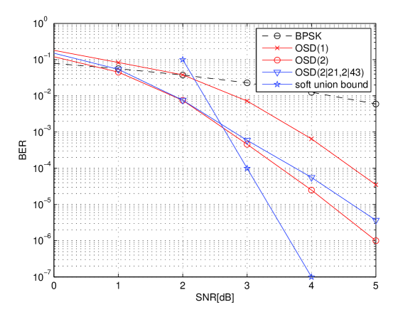
Figure 4: The BER of the $(128,64,22)$ BCH code over an AWGN channel.

We compare the number of binary operations (BOPS) and the number of floating point operations (FLOPS) required to execute the decoding algorithms proposed in this paper. Assuming a $(N,K,{d_{\mathrm{min}}})$ code, the complexity of the OSD and the POSD are given in Table I and Table II. The implementation complexity expressions in Table I for $\mathrm{OSD}(I)$ are from the reference [3]. For example, the OSD decoding of the BCH code $(128,64,22)$ requires at least $1152$ FLOPS and $528448$ BOPS to find the MRIPs and to obtain the corresponding equivalent generator matrix in a row echelon form. All this complexity can be completely avoided by assuming the partial ordering in the POSD decoding. The number of the test error patterns is $L=2080$ for $\mathrm{OSD}(2)$, and $L=1177$ for $\mathrm{OSD}(2,2)$ with $K_{1}=21$ and $K_{2}=43$ whereas the coding gain of $\mathrm{OSD}(2)$ can be only slightly better than the coding gain of $\mathrm{OSD}(2,2)$; see, for example, Fig. 4. Hence, the overall complexity of the OSD-based schemes can be substantially reduced by avoiding the Gauss (Gauss-Jordan) elimination.

V Performance Analysis

Recall that we assume a memoryless communication channel as described in Section II. We derive the probability $\mathrm{Pr}\!\left\{\hat{\mathbf{c}}_{0}\in\mathcal{E}_{L}\right\}$ in (9) that the error pattern $\hat{\mathbf{c}}_{0}$ observed at the receiver after transmission of the codeword $\mathbf{c}_{\mathrm{Tx}}=\mathbf{0}$ is an element of the chosen decoding list $\mathcal{E}_{L}$. The derivation relies on the following generalization of Lemma 3 in [3].

Lemma 2

For any ordering of the $N$ received bits, consider the $I$ bit positions $\mathcal{I}\subseteq\{1,2,\cdots,N\}$, and the $\binom{I}{I_{1}}$ subsets $\mathcal{I}_{1}\subseteq\mathcal{I}$ of $I_{1}\leq I\leq N$ bit positions. Then, the total probability of the $I_{1}$ bit errors within the $I$ bits can be calculated as,

$$\sum_{\mathcal{I}_{1}:\ |\mathcal{I}_{1}|=I_{1}}\mathrm{P}(\mathcal{I}_{1})=\binom{I}{I_{1}}\,p_{0}^{I_{1}}$$

where $p_{0}$ is the probability of bit error corresponding to the bit positions $\mathcal{I}$.

Proof:

The ordering of the chosen $I$ bits given by the set $\mathcal{I}$ is irrelevant since all subsets $\mathcal{I}_{1}$ of $I_{1}$ errors within the $I$ bits $\mathcal{I}$ are considered. Consequently, the bit errors in the set $\mathcal{I}$ can be considered to be independent having the equal probability denoted as $p_{0}$. ∎

Using Lemma 2, we observe that the lists of error patterns (10) and (12) are constructed, so that the ordering of bits within the segments is irrelevant. Then, the bit errors in a given segment can be considered to be conditionally independent. This observation is formulated as the following corollary of Lemma 2.

Corollary 1

For the $\mathrm{OSD}(I)$ and the list of error patterns (10), the bit errors in the MRIPs can be considered as conditionally independent. Similarly, for the $\mathrm{POSD}(I_{1},I_{2})$ and the list of error patterns (12), the bit errors in the two segments can be considered as conditionally independent.

Thus, the bit errors in Corollary 1 are independent conditioned on the particular segment being considered as shown next.

Let $\mathrm{P}_{0}$ be the bit error probability of the MRIPs for the $\mathrm{OSD}(I)$ decoding. Similarly, let $\mathrm{P}_{1}$ and $\mathrm{P}_{2}$ be the bit error probabilities in the first and the second segments of the $\mathrm{OSD}(I_{1},I_{2})$ decoding, respectively. Denote the auxiliary variables, $v_{1}=|\tilde{r}_{K_{1}}|$, $v_{2}=|\tilde{r}_{K_{1}+1}|$, and $v_{3}=|\tilde{r}_{K+1}|$ of the order statistics (3), and let $u\equiv|r_{i}|$, $i=1,2,\cdots,K$. Hence, always, $v_{1}\geq v_{2}$, and, for simplicity, ignoring the second permutation $\lambda^{\prime\prime}$, also, $v_{2}\geq v_{3}$. The probability of bit error $\mathrm{P}_{0}$ for the MRIPs is calculated as,

$$\mathrm{P}_{0}=\mathrm{E}_{u}\!\left[\int_{0}^{u}\frac{f_{v_{3}}(v)}{1-F_{u}(v)}{\mathrm{d}}v\right]$$

where $\mathrm{E}_{u}\!\left[\cdot\right]$ denotes the expectation w.r.t. (with respect to) $u$, $f_{v_{3}}(v)$ is the PDF of the $(K+1)$-th order statistic in (3), and $F_{u}(v)$ is the cumulative distribution function (CDF) of the magnitude (the absolute value) of the reliability of the received bits (before ordering). Similarly, the probability of bit error $\mathrm{P}_{1}$ for the first segment is calculated as,

$$\mathrm{P}_{1}=\mathrm{E}_{u}\!\left[\int_{0}^{u}\frac{f_{v_{2}}(v)}{1-F_{u}(v)}{\mathrm{d}}v\right]$$

where $f_{v_{2}}(v)$ is the PDF of the $(K_{1}+1)$-th order statistic in (3). The probability of bit error $\mathrm{P}_{2}$ for the second segment is calculated as,

$$\mathrm{P}_{2}=\mathrm{E}_{u}\!\left[\int_{0}^{u}\!\int_{u}^{\infty}\frac{f_{v_{1}}(v)f_{v_{3}}(v^{\prime})}{(F_{u}(v)-F_{u}(v^{\prime}))(1-F_{v_{1}}(v^{\prime}))}{\mathrm{d}}v{\mathrm{d}}v^{\prime}\right]$$

where $f_{v_{1}}(v)$ and $F_{v_{1}}(v^{\prime})$ is the PDF and the CDF of the $K_{1}$-th order statistic in (3), respectively. The values of the probabilities $\mathrm{P}_{0}$, $\mathrm{P}_{1}$ and $\mathrm{P}_{2}$ have to be evaluated by numerical integration. Finally, we use Lemma 2 and substitute the probabilities $\mathrm{P}_{0}$, $\mathrm{P}_{1}$ and $\mathrm{P}_{2}$ for $p_{0}$ to calculate the probability $\mathrm{Pr}\!\left\{\hat{\mathbf{c}}_{0}\in\mathcal{E}_{L}\right\}$ of the error patterns in the list $\mathcal{E}_{L}$.

VI Numerical Examples

We use computer simulations to compare the BER performances of the proposed soft-decision decoding schemes. All the block codes considered are linear and systematic.

The BER of the $(31,16,7)$ BCH code over an AWGN channel is shown in Fig. 2 assuming $\mathrm{ISD}(2)$ and $\mathrm{ISD}(3)$ with $K=16$ having $137$ and $697$ test error patterns, respectively, and assuming $\mathrm{POSD}(1,3)$ and $\mathrm{POSD}(2,3)$ with $K_{1}=6$ and $K_{2}=10$ having $183$ and $198$ test error patterns, respectively. We observe that $\mathrm{POSD}(1,3)$ achieves the same BER as $\mathrm{ISD}(3)$ while using much less error patterns which represents the gain of the ordering of the received information bits into two segments. At the BER of $10^{-4}$, $\mathrm{POSD}(1,3)$ outperforms $\mathrm{ISD}(2)$ by $1.1$ dB using approximately $50\%$ more test error patterns. Thus, the $\mathrm{POSD}(1,3)$ decoding provides $2.3$ dB coding gain with the small implementation complexity at the expense of $2$ dB loss compared to the ML decoding.

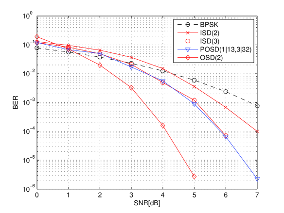
Figure 3: The BER of the $(63,45,14)$ BCH code over an AWGN channel.

Fig. 3 shows the BER of the $(63,45,14)$ BCH code over an AWGN channel. The number of test error patterns for the $\mathrm{ISD}(2)$, $\mathrm{ISD}(3)$, $\mathrm{POSD}(1,3)$ and $\mathrm{OSD}(2)$ decodings are $1036$, $15226$, $5503$ and $1036$, respectively. We observe from Fig. 3 that $\mathrm{ISD}(3)$ has the same BER as $\mathrm{POSD}(1,3)$ with two segments of $K_{1}=13$ and $K_{2}=32$ bits. However, especially for the high rate codes (i.e. of rates greater than $1/2$), one has to also consider the complexity of the Gauss elimination to obtain the row echelon form of the generator matrix for the OSD. For example, the Gauss elimination for the $(63,45,14)$ code requires approximately $20,400$ BOPS; cf. Table I.

The BER of the $(128,64,22)$ BCH code over an AWGN channel is shown in Fig. 4 assuming $\mathrm{OSD}(1)$ and $\mathrm{OSD}(2)$ with $K=64$, and assuming $\mathrm{OSD}(2,2)$ with $K_{1}=21$ and $K_{2}=43$. The number of test error patterns for the $\mathrm{OSD}(1)$, $\mathrm{OSD}(2)$ and $\mathrm{OSD}(2,2)$ decodings are $64$, $2081$ and $1179$. A truncated union bound of the BER in Fig. 4 is used to indicate the ML performance [14, Ch. 10]. We observe that both $\mathrm{OSD}(2)$ and $\mathrm{OSD}(2,2)$ have the same BER performance for the BER values larger than $10^{-3}$, and $OSD(2)$ outperforms $\mathrm{OSD}(2,2)$ by at most $0.5$ dB for the small values of the SNR. Our numerical results indicate that, in general, $\mathrm{OSD}(2,2)$ decoding can achieve approximately the same BER as $\mathrm{OSD}(2)$ for small to medium SNR while using about $50\%$ less error patterns. Thus, a slightly smaller coding gain (less than $0.5$dB) of $\mathrm{OSD}(2,2)$ in comparison with $\mathrm{OSD}(2)$ at larger values of the SNR is well-compensated for by the reduced decoding complexity. More importantly, $\mathrm{OSD}(2,2)$ can trade-off the BER performance and the decoding complexity between those provided by $\mathrm{OSD}(1)$ and $\mathrm{OSD}(2)$, especially at larger values of SNR.

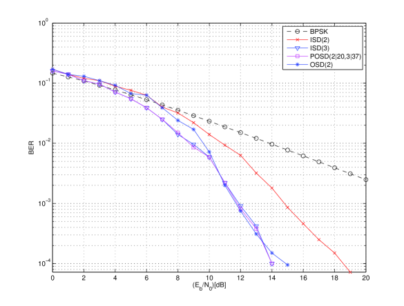
Figure 6: The BER of the $(64,57,4)$ BCH coded over a Rayleigh fading channel.

The BER of the $(31,16,7)$ BCH code over a fast Rayleigh fading channel is shown in Fig. 5. We assume the same decoding schemes as in Fig. 2. The $\mathrm{POSD}(1,3)$ decoding with $183$ error patterns achieves the coding gain of $17$ dB over an uncoded system, the coding gain of $4$ dB over $\mathrm{ISD}(2)$ with $137$ error patterns, and it has the same BER as $\mathrm{OSD}(3)$ with $697$ error patterns. The BER of the high rate BCH code $(64,57,4)$ over a fast Rayleigh channel is shown in Fig. 6. In this case, the number of test error patterns for the $\mathrm{ISD}(2)$, $\mathrm{ISD}(3)$, $\mathrm{POSD}(2,3)$ and $\mathrm{OSD}(2)$ decoding is $1654$, $30914$, $8685$ and $1654$, respectively. We observe that, for small to medium SNR, $\mathrm{POSD}(2,3)$ which does not require the Gauss elimination (corresponding to approximately $3,000$ BOPS) outperforms $\mathrm{OSD}(2)$ by $1$dB whereas, for large SNR values, these two decoding schemes achieve approximately the same BER performance.

VII Conclusions

Low-complexity soft-decision decoding techniques employing a list of the test error patterns for linear binary block codes of small to medium block length were investigated. The optimum and suboptimum construction of the list of error patterns was developed. Some properties of the joint probability of error of the received bits after ordering were derived. The original OSD algorithm was generalized by assuming a segmentation of the MRIPs. The segmentation of the MRIPs was shown to overcome several drawbacks of the original OSD and to enable flexibility for devising new decoding strategies. The decoding complexity of the OSD-based decoding algorithms was reduced further by avoiding the Gauss (or the Gauss Jordan) elimination using the partial ordering of the received bits in the POSD decoding. The performance analysis was concerned with the problem of finding the probability of the test error patterns contained in the decoding list. The BER performance and the decoding complexity of the proposed decoding techniques were compared by extensive computer simulations. Numerical examples demonstrated excellent flexibility of the proposed decoding schemes to trade-off the BER performance and the decoding complexity. In some cases, both the BER performance as well as the decoding complexity of the segmentation-based OSD were found to be improved compared to the original OSD.

Appendix

We derive the probabilities $\mathrm{P}_{0}$, $\mathrm{P}_{1}$ and $\mathrm{P}_{2}$ in Section V. Without loss of generality, we assume that the all-ones codeword was transmitted, i.e., $x_{i}=-1$ for $\forall i$. Then, after ordering, the $i$-th received bit, $i=1,2,\cdots,N$, is in error, provided that $\tilde{r}_{i}>0$. The probability of bit error $\mathrm{P}_{0}$ for the MRIPs is obtained as,

$$\mathrm{P}_{0}=\int_{0}^{\infty}\!\int_{0}^{\infty}f_{u}(u|u\geq v_{3})f_{v_{3}}(v_{3}){\mathrm{d}}v_{3}{\mathrm{d}}u$$

where the conditional PDF [16],

$$f_{u}(u|u\geq v_{3})=\left\{\begin{array}[]{cc}\frac{f_{u}(u)}{1-F_{u}(v_{3})}&u\geq v_{3}\\ 0&u<v_{3}\end{array}\right.$$

and $f_{u}(u)$ and $F_{u}(v_{3})$ are the PDF and the CDF of the reliability of the received bits, respectively, so that,

$$\mathrm{P}_{0}=\int_{0}^{\infty}\!f_{u}(u)\int_{0}^{u}\frac{f_{v_{3}}(v_{3})}{1-F_{u}(v_{3})}{\mathrm{d}}v_{3}{\mathrm{d}}u.$$

Similarly, the probability of bit error $\mathrm{P}_{1}$ for the first segment is calculated as,

$$\mathrm{P}_{1} = \int_{0}^{\infty}\int_{0}^{\infty}f_{u}(u|u\geq v_{2})f_{v_{2}}(v_{2}){\mathrm{d}}v_{2}{\mathrm{d}}u$$

$$= \int_{0}^{\infty}\!f_{u}(u)\int_{0}^{u}\frac{f_{v_{2}}(v_{2})}{1-F_{u}(v_{2})}{\mathrm{d}}v_{2}{\mathrm{d}}u.$$

The probability of bit error $\mathrm{P}_{2}$ for the second segment is calculated as,

$$\mathrm{P}_{2}=\int_{0}^{\infty}\int_{0}^{\infty}\!\int_{0}^{\infty}f_{u}(u|v_{1}\geq u\geq v_{3})f_{v_{1},v_{3}}(v_{1},v_{3}){\mathrm{d}}v_{1}{\mathrm{d}}v_{3}{\mathrm{d}}u$$

where the conditional PDF,

$$f_{u}(u|v_{1}\geq u\geq v_{3})=\left\{\begin{array}[]{cc}\frac{f_{u}(u)}{F_{u}(v_{1})-F_{u}(v_{3})}&v_{1}\geq u\geq v_{3}\\ 0&\mbox{otherwise}\end{array}\right.$$

and the joint PDF of the order statistics $v_{1}\geq v_{3}$ is,

$$f_{v_{1},v_{3}}(v_{1},v_{3})=\left\{\begin{array}[]{cc}\frac{f_{v_{1}}(v_{1})}{1-F_{v_{1}}(v_{3})}f_{v_{3}}(v_{3})&v_{1}\geq v_{3}\\ 0&v_{1}<v_{3}\end{array}\right.$$

and thus,

$$\mathrm{P}_{2}=\int_{0}^{\infty}f_{u}(u)\int_{0}^{u}\!\int_{u}^{\infty}\frac{f_{v_{1}}(v)f_{v_{3}}(v^{\prime})}{(F_{u}(v)-F_{u}(v^{\prime}))(1-F_{v_{1}}(v^{\prime}))}{\mathrm{d}}v{\mathrm{d}}v^{\prime}{\mathrm{d}}u.$$

TABLE I: Implementation Complexity of the OSD and the POSD

$\mathrm{OSD}(I_{1})$ and $\mathrm{OSD}(I_{1},I_{2})$
operation	complexity
$\mathbf{r}$	$2N$ FLOPS
$\tilde{\mathbf{r}}^{\prime}$	$N\log_{2}(N)$ FLOPS
Gauss el. $\mathbf{G}^{\prime}$	$N\min(K,N-K)^{2}$ BOPS
$\tilde{\mathbf{r}}^{\prime\prime}$	$K+K(N-K)$ BOPS
$\mathrm{POSD}(I_{1})\equiv\mathrm{ISD}(I_{1})$
operation	complexity
$\mathbf{r}$	$2N$ FLOPS
$\tilde{\mathbf{r}}^{\prime}$	$0$ BOPS
$\mathrm{POSD}(I_{1},I_{2})$
operation	complexity
$\mathbf{r}$	$2N$ FLOPS
$\tilde{\mathbf{r}}^{\prime}$	$K\log_{2}(K)$ FLOPS

TABLE II: Decoding List Sizes for the OSD and the POSD

$\mathrm{OSD}(I)$	$\sum_{l=0}^{I}\binom{K}{l}$
$\mathrm{OSD}(I_{1},I_{2})$	$\sum_{l=0}^{I_{1}}\binom{K_{1}}{l}+\sum_{l=0}^{I_{2}}\binom{K_{2}}{l}$
$\mathrm{POSD}(I)\equiv\mathrm{ISD}(I)$	$\sum_{l=0}^{I}\binom{K}{l}$
$\mathrm{POSD}(I_{1},I_{2})$	$\sum_{l=0}^{I_{1}}\binom{K_{1}}{l}+\sum_{l=0}^{I_{2}}\binom{K_{2}}{l}$

Figure 1: The system model and an equivalent vector channel with the binary vector input $\mathbf{c}$ and the vector soft-output $\tilde{\mathbf{r}}_{0}$.

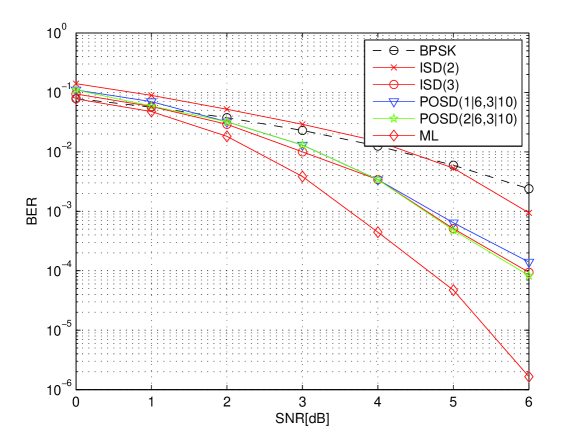
Figure 2: The BER of the $(31,16,7)$ BCH code over an AWGN channel.

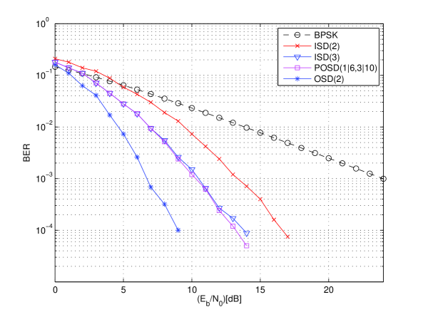
Figure 5: The BER of the $(31,16,7)$ BCH code over a Rayleigh fading channel.

References

- [1] H. Yagi, “A study on complexity reduction of the reliability-based maximum likelihood decoding algorithm for block codes,” PhD dissertation, Waseda University, 2005.
- [2] B. Dorsch, “A decoding algorithm for binary block codes and -ary output channels,” IEEE Trans. Inf. Theory, vol. 20, pp. 391-394, 1974.
- [3] M. P. C. Fossorier and S. Lin, “Soft-decision decoding of linear block codes based on ordered statistics,” IEEE Trans. Inf. Theory, vol. 41, pp. 1379-1396. Sept. 1995.
- [4] D. Gazelle and J. Snyders, “Reliability-based code-search algorithms for maximum-likelihood decoding of block codes,” IEEE Trans. Inf. Theory, vol. 43, pp. 239-249, Jan. 1997.
- [5] A. Kabat, F. Guilloud and R. Pyndiah, “New approach to order statistics decoding of long linear block codes,” in Proc. Globecom, pp. 1467-1471, Nov. 2007.
- [6] H. Yagi, T. Matsushima and S. Hirasawa, “Fast algorithm for generating candidate codewords in reliability-based maximum likelihood decoding,” IEICE Trans. Fundamentals, vol. E89-A, pp. 2676-2683, Oct. 2006.
- [7] M. Fossorier and S. Lin, “Computationally efficient soft decision decoding of linear block codes based on ordered statistics,” IEEE Trans. Inf. Theory, vol. 42, pp. 738-750, May 1996.
- [8] M. Fossorier, “Reliability-based soft-decision decoding with iterative information set reduction,” IEEE Trans. Inf. Theory., vol. 48, no. 12, pp. 3101-3106, Dec. 2002.
- [9] W. Jin and M. Fossorier, “Reliability based soft decision decoding with multiple biases,” IEEE Trans. Inf. Theory, vol. 53, no. 1, pp. 105-119, Jan. 2007.
- [10] A. Valembois and M. Fossorier, “Sort-and-match algorithm for soft-decision decoding,” IEEE Trans. Inf. Theory, vol. 45, pp. 2333-2338, Nov. 1999.
- [11] A. Valembois and M. Fossorier, “Box and match techniques applied to soft decision decoding,” IEEE Trans. Inf. Theory, vol. 50, no. 5, pp. 796-810, May 2004.
- [12] M. El-Khamy, H. Vialko, B. Hassibi and R. McEliecce,“Performance of sphere decoding of block codes,” IEEE Trans. Comms., vol. 57, pp. 2940–2950, Oct. 2009.
- [13] H. Vikalo and B. Hassibi, “On joint detection and decoding of linear block codes on Gaussian vector channels,” IEEE Trans. Signal Proc., vol. 54, pp. 3330–3342, Sep. 2006.
- [14] S. Benedetto and E. Biglieri, Principles of Digital Transmission With Wireless Applications, Kluwer Academic, 1999.
- [15] S. Lin and D. J. Costello, Error Control Coding: Fundamentals and Applications, Prentice-Hall, 1983.
- [16] A. Papoulis and S. U. Pillai, Probability, Random Variables, and Stochastic Processes, 4th Ed., McGraw-Hill, 2002.