Cosmological effects on the observed flux and fluence distributions of gamma-ray bursts:
Are the most distant bursts in general the faintest ones?

Abstract

Context. Several claims have been put forward that an essential fraction of long-duration BATSE gamma-ray bursts should lie at redshifts larger than 5. This point-of-view follows from the natural assumption that fainter objects should, on average, lie at larger redshifts. However, redshifts larger than 5 are rare for bursts observed by Swift, seemingly contradicting the BATSE estimates.

Aims. The purpose of this article is to clarify this contradiction.

Methods. We derive the cosmological relationships between the observed and emitted quantities, and we arrive at a prediction that can be tested on the ensembles of bursts with determined redshifts. This analysis is independent on the assumed cosmology, on the observational biases, as well as on any gamma-ray burst model. Four different samples are studied: 8 BATSE bursts with redshifts, 13 bursts with derived pseudo-redshifts, 134 Swift bursts with redshifts, and 6 Fermi bursts with redshifts.

Results. The controversy can be explained by the fact that apparently fainter bursts need not, in general, lie at large redshifts. Such a behaviour is possible, when the luminosities (or emitted energies) in a sample of bursts increase more than the dimming of the observed values with redshift. In such a case $dP(z)/dz>0$ can hold, where $P(z)$ is either the peak-flux or the fluence. All four different samples of the long bursts suggest that this is really the case. This also means that the hundreds of faint, long-duration BATSE bursts need not lie at high redshifts, and that the observed redshift distribution of long Swift bursts might actually represent the actual distribution.

1 Introduction

Until the last years, the redshift distribution of gamma-ray bursts (GRBs) has only been poorly known. For example, the Burst and Transient Source Experiment (BATSE) instrument on Compton Gamma Ray Observatory detected around 2700 GRBs, but only a few of these have directly measured redshifts from the afterglow (AG) observations (Schaefer (2003); Piran (2004)). During the last couple of years the situation has improved, mainly due to the observations made by the Swift satellite. There are already dozens of directly determined redshifts (Mészáros (2006)). Nevertheless, this sample is only a small fraction of the, in total, thousands of detected bursts.

Beside the direct determination of redshifts from the AGs, there are several indirect methods, which utilize the gamma-ray data alone. In essence, there are two different methods which provide such determinations. The first one makes only statistical estimations; the fraction of bursts in a given redshift interval is deduced. The second one determines an actual value of the redshift for a given GRB (”pseudo-redshift”).

Already at the early 1990’s, that is, far before the observation of any AG, and when even the cosmological origin was in doubt, there were estimations made in the sense of the first method (see, e.g., Paczyński (1992) and the references therein). In Mészáros & Mészáros (1996) a statistical study indicated that a fraction of GRBs should be at very large redshifts (up to $z\simeq 20$). In addition, there was no evidence for the termination of the increase of the numbers of GRBs for $z>5$ (see also Mészáros & Mészáros (1995); Horváth et al. (1996), and Reichart & Mészáros (1997)). In other words, an essential fraction (a few or a few tens of %) of GRBs should be in the redshift interval $5<z<20$. Again using this type of estimation, Lin et al. (2004) claims that even the majority of bursts should be at these high redshifts.

The estimations of the pseudo-redshifts in the sense of the second method are more recent. Ramirez-Ruiz & Fenimore (2000), Reichart et al. (2001), Schaefer et al. (2001) and Lloyd-Ronning et al. (2002) developed a method allowing to obtain from the so-called variability the intrinsic luminosity of a GRB, and then from the measured flux its redshift. The redshifts of hundred of bursts were obtained by this method. Nevertheless, the obtained pseudo-redshifts are in doubt, because there is an $(1+z)$ factor error in the cosmological formulas (Norris (2004), Band et al. 2004). Other authors also query these redshifts (e.g., Guidorzi et al. (2005)). Norris et al. (2000) found another relation between the spectral lag and the luminosity. This method seems to be a better one (Schaefer et al. (2001); Norris (2002); Ryde et al. (2005)), and led to the estimation of $\sim 1200$ burst redshifts. Remarkably, again, an essential fraction of long GRBs should have $z>5$, and the redshift distribution should peak at $z\sim 10$. A continuation of this method (Band et al. (2004), Norris 2004), which corrected the $(1+z)$ error in Norris (2002), gave smaller redshifts on average, but the percentage of long GRBs at $z>5$ remains open. Bagoly et al. (2003) developed a different method allowing to obtain the redshifts from the gamma spectra for 343 bright GRBs. Due to the two-fold character of the estimation, the fraction of GRBs at $z>5$ remains further open. No doubt has yet emerged concerning this method. Atteia (2003) also proposed a method in a similar sense for bright bursts. Other methods of such estimations also exist (Amati et al. (2002); Ghirlanda et al. (2005)). These pseudo-redshift estimations (for a survey see, e.g. Sect.2.6 of Mészáros (2006)) give the results that even bright GRBs should be at redshifts $z\sim(1-5)$. For faint bursts in the BATSE data set (i.e. for GRBs with peak-fluxes smaller than $\simeq 1$ photon/(cm²s)) one hardly can have good pseudo-redshift estimations, but on average they are expected to be at larger redshifts, using the natural assumption that these bursts are observationally fainter due to their larger distances. Hence, it is remarkable that all these pseudo-redshift estimations also supports the expectation, similarly to the results of the first method, that an essential fraction of GRBs is at very high redshifts.

Contrary to these estimations for the BATSE data set, only five long bursts with $z>5$ bursts have yet been detected from direct redshift measurements from AGs using more recent satellites. In addition, the majority of measured $z$-s are around $z=2-3$, and there is a clear decreasing tendency towards the larger redshifts. In other words, the redshifts of GRBs detected by the Swift satellite do not support the BATSE redshift estimations; the redshifts of GRBs detected by the non-Swift satellites are on average even at smaller redshifts (Bagoly et al. (2006)).

This can be interpreted in two essentially different ways. The first possibility is that a large fraction (a few tens of % or even the majority) of GRBs are at very high redshifts (at $z>5$ or so). In such case these bursts should mainly be seen only in the gamma-ray band due to some observational selection (Lamb & Reichart (2000)). The second possibility is that the AG data reflect the true distribution of bursts at high redshifts, and bursts at $z>5$ are really very rare. In this case, however, there has to be something wrong in the estimations of redshifts from the gamma-ray data alone. Since observational selections for AG detections of bursts at $z>5$ cannot be excluded (Lamb & Reichart (2000)), the first point-of-view could be also quite realistic.

The purpose of this paper is to point out some statistical properties of the GRBs, which may support the second possibility. Section 2 discusses these properties theoretically. In sections 3 and 4 we discuss the impact of such a behaviour on several observed burst samples. Section 5 summarizes the results of paper.

2 Theoretical considerations

2.1 The general consideration

Using the standard cosmological theory and some simple statistical considerations, we will now show that, under some conditions, apparently fainter bursts might very well be at smaller redshifts compared to the brighter ones.

As shown by Mészáros & Mészáros (1995), if there are given two photon-energies $E_{1}$ and $E_{2}$, where $E_{1}<E_{2}$, then the flux $F$ (in units photons/(cm²s)) of the photons with energies $E_{1}\leq E\leq E_{2}$ detected from a GRB having a redshift $z$ is given by

$$F_{\mathrm{ph}}(z)=\frac{(1+z)\tilde{L}_{\mathrm{ph}}(z)}{4\pi d_{\mathrm{l}}(z)^{2}}=\frac{\tilde{L}_{\mathrm{ph}}(z)}{4\pi d_{\mathrm{M}}(z)^{2}(1+z)},$$ (1)

where $\tilde{L}_{\mathrm{ph}}(z)$ is the isotropic luminosity of a GRB (in units photons/s) between the energy range $E_{1}(1+z)\leq E\leq E_{2}(1+z)$, and $d_{\mathrm{l}}(z)$ is the luminosity distance of the source. The reason of the notation $\tilde{L}(z)$, instead of the simple $L(z)$, is that $L(z)$ should mean the luminosity from $E_{1}\leq E\leq E_{2}$ (Mészáros et al. (2006)). One has $d_{\mathrm{l}}(z)=(1+z)d_{\mathrm{M}}(z)$, where $d_{\mathrm{M}}(z)$ is the proper motion distance of the GRB, given by the standard cosmological formula (Carroll et al. (1992)), and depends on the cosmological parameters $H_{0}$ (Hubble-constant), $\Omega_{\mathrm{M}}$ (the ratio of the matter density and the critical density), and $\Omega_{\mathrm{\Lambda}}=3\lambda c^{2}/(3H_{0}^{2})$ ($\lambda$ is the cosmological constant, $c$ is the velocity of light). In energy units one may write $F_{\mathrm{en}}(z)=\overline{E}F_{\mathrm{ph}}(z)$ and $\tilde{L}_{\mathrm{en}}(z)=(1+z)\overline{E}\tilde{L}_{\mathrm{ph}}(z)$, where $\overline{E}$ ($E_{1}<\overline{E}<E_{2}$) is a typical photon energy ensuring that the flux $F_{\mathrm{en}}(z)$ has the dimension erg/(cm²s). $\tilde{L}_{\mathrm{en}}(z)$ in erg/s unit gives the luminosity in the interval $E_{1}(1+z)\leq E\leq E_{2}(1+z)$. Except for an $(1+z)$ factor the situation is the same, when considering the fluence. Hence, in the general case, we have

$$P(z)=\frac{(1+z)^{N}\tilde{L}(z)}{4\pi d_{\mathrm{l}}(z)^{2}},$$ (2)

where $P(z)$ is either the fluence or the flux, and $\tilde{L}(z)$ is either the emitted isotropic total number of photons, or the isotropic total emitted energy or the luminosity. The following values of $N$ can be used: $N=0$ if the flux is taken in energy units erg/(cm²s) and $\tilde{L}$ is the luminosity with dimension erg/s; $N=1$ if either the flux and luminosity are in photon units, or the fluence in energy units and the total energy are taken; $N=2$ if the total number of photons are considered. All this means that for a given GRB - for which redshift, flux and fluence are measured - Eq.(2) defines immediately $\tilde{L}(z)$, which is then either the isotropic total emitted energy or the luminosity in the interval $E_{1}(1+z)\leq E\leq E_{2}(1+z)$. Hence, $\tilde{L}(z)$ is from the range $E_{1}(1+z)\leq E\leq E_{2}(1+z)$ and not from $E_{1}\leq E\leq E_{2}$.

Let us have a measured value of $P(z)$. Fixing this $P(z)$ Eq.(2) defines a functional relationship between the redshift $z$ and $\tilde{L}(z)$. For its transformation into the real intrinsic luminosities $L(z)$ the beaming must be taken into account as well (Lee et al. (2000); Ryde et al. (2005); Bagoly & Veres 2009a ; Petrosian et al. (2009); Bagoly & Veres 2009b ; Butler et al. (2010)). Additionally, we need to study the dependence of the obtained $\tilde{L}(z)$ on $z$, and to determine the real luminosities $L(z)$ by the K-corrections (Mészáros (2006)). It is not the aim of this paper to solve the transformation of $\tilde{L}(z)$ into $L(z)$. The purpose of this paper is to study the functional relationship among $P(z)$, $z$ and $\tilde{L}(z)$.

Using the proper motion distance $d_{\mathrm{M}}(z)$ Eq.(2) can be reordered as

$$4\pi d_{\mathrm{M}}(z)^{2}(1+z)^{2-N}P(z)=\tilde{L}(z).$$ (3)

The proper motion distance $d_{\mathrm{M}}(z)$ is bounded as $z\rightarrow\infty$ (Weinberg 1972, Chapter. 14.4.). This finiteness of the proper motion distance is fulfilled for any $H_{0},\;\Omega_{\mathrm{M}}$ and $\Omega_{\mathrm{\Lambda}}$. Hence, $\tilde{L}(z)$ is a monotonically increasing function of the redshift along with $(1+z)^{2-N}$ for the fixed $P(z)=P_{0}$ and for the given value of $N\leq 1$. It means $z_{1}<z_{2}$ implies $\tilde{L}(z_{1})<\tilde{L}(z_{2})$. Expressing this result in other words: the more distant and brighter sources may give the same observed value of $P_{0}$. Now, if a source at $z_{2}$ has a $\tilde{L}’>\tilde{L}(z_{2})$, its observed value $P^{\prime}_{obs}$ will have $P^{\prime}_{obs}>P_{0}$, i.e. it becomes apparently brighter despite its greater redshift than that of the source at $z_{1}$. The probability of the occurrence this kind of inversion depends on $f(\tilde{L}|z)$, on the conditional probability density of $\tilde{L}$ assuming $z$ is given, and on the spatial density of the objects.

It is obvious from Eq.(3) that for the increasing $z$ the $\tilde{L}(z)$ is also increasing. This effect gives a bias (Lee et al. (2000); Bagoly & Veres 2009a ; Petrosian et al. (2009); Bagoly & Veres 2009b ; Butler et al. (2010)) towards the higher $\tilde{L}(z)$ values among GRBs observed above a given detection threshold. [These questions are discussed in detail mainly by Petrosian et al. (2009).] There can be also that $\tilde{L}(z)$ is increasing with $z$ due to the metallicity evolution (Wolf & Podsiadlowski (2007)). There can be also an intrinsic evolution of the $L(z)$ itself in the energy range $[E_{1},E_{2}]$. Hence, keeping all this in mind, $\tilde{L}(z)$ can well be increasing on $z$, and the inverse behaviour can also occur.

2.2 A special assumption

Assume now that we have $\tilde{L}(z)\propto(1+z)^{\mathrm{q}}$, where $q$ is real number, and this relation holds for any $0<z<\infty$. This means that it holds $\tilde{L}(z)=\tilde{L}_{0}(1+z)^{\mathrm{q}}$, where $\tilde{L}(z=0)=\tilde{L}_{0}$. Of course, this special assumption is a loss of generality, because $\tilde{L}(z)$ can be really a function of $z$, but in general it need not have this special form. In addition, to calculate $\tilde{L}(z)$ the cosmological parameters must be specified, which is a further loss of generality. Nevertheless, if this special assumption is taken, the inverse behavior may well be demonstrated.

If $(N+q)>2$, then one has a highly interesting mathematical behaviour of the function $P(z)$ (Eq.2). For $z\ll 0.1$, $P(z)$ decreases as $z^{-2}$, that is, larger redshifts gives smaller fluxes or fluences as expected. However, after some $z=z_{\mathrm{turn}}$ this behavior must change, because as $z$ tends to $\infty$, the function $(1+z)^{\mathrm{N}}\tilde{L}/d_{\mathrm{l}}^{2}$ tends to infinity following $\propto(1+z)^{\mathrm{N+q-2}}$. In other words, for $z>z_{\mathrm{turn}}$ as redshift increases, the measured $P(z)$ will also increase. Equivalently stated, ”fainter bursts are closer to us”. The possibility of this ”inverse” behaviour is quite remarkable. It is important to note that the existence of a $z_{\mathrm{turn}}$ is exclusively determined by the value $q$, and the necessary and sufficient condition for it is given by the inequality $(N+q)>2$. For the existence of a $z_{\mathrm{turn}}$ the values $H_{0},\Omega_{\mathrm{M}}$ and $\Omega_{\mathrm{\Lambda}}$ are unimportant. The value of $z_{\mathrm{turn}}$ can vary depending on the choice of the $\Omega$ parameters, but, however, its existence or non-existence is unaffected.

Moreover, the value of $z_{\mathrm{turn}}$ itself is independent on the Hubble-constant $H_{0}$. This can be seen as follows. To find $z_{\mathrm{turn}}$ one must simply search for the minimum of the function $Q(z)=(1+z)^{N+q}/d_{\mathrm{l}}(z)^{2}$, that is, when $dQ(z)/dz=0$. But, trivially, $Q(z)$ and $Q(z)/H_{0}^{2}$ have the same minimum.

The solution of the equation $dQ(z)/dz=0$ must be found numerically for the general case of Omega parameters. The left panel of Fig.1 shows the function $Q(z)$ for $\Omega_{\mathrm{M}}=0.27$ and $\Omega_{\mathrm{\Lambda}}=0.73$. For $\Omega_{\mathrm{\Lambda}}=0$ it can be found analytically, because $d_{\mathrm{M}}(z)$ is then an analytical function. For $\Omega_{\mathrm{M}}=1$ and $\Omega_{\mathrm{\Lambda}}=0$ the condition $dQ(z)/dz=0$ is easily solvable. For this special case one has to search for the minimum of function

$$\frac{(1+z)^{N+q-2}}{(1-(1+z)^{-1/2})^{2}},$$ (4)

because here $d_{\mathrm{M}}=(2c/H_{0})/(1-(1+z)^{-1/2})$. Then one has

$$z_{\mathrm{turn}}=\Bigl{(}\frac{{N+q-1}}{N+q-2}\Bigr{)}^{2}-1.$$ (5)

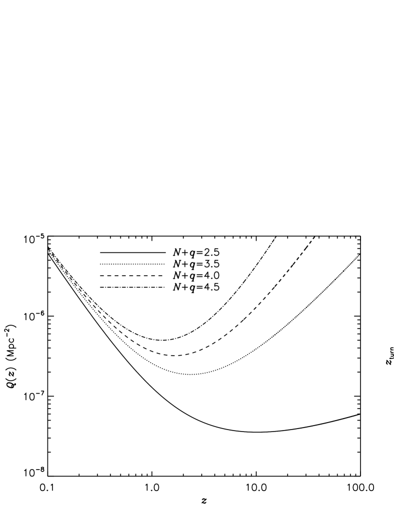
Figure 1: Left panel: Function $Q(z)$ for $\Omega_{\mathrm{M}}=0.27$ and $\Omega_{\mathrm{\Lambda}}=0.73$. Right panel: Dependence of $z_{\mathrm{turn}}$ on $q$ for $\Omega_{\mathrm{M}}=0.27$ and $\Omega_{\mathrm{\Lambda}}=0.73$.

3 The samples

3.1 The choice of burst samples

The frequency of the occurrence $\tilde{L}(z_{1})<\tilde{L}(z_{2})$ at $z_{1}<z_{2}$, but for their observed values $P(z_{1})<P(z_{2})$, i.e. the more distant GRB is apparently brighter for the observer, can be verified on a sample for which there are well-defined redshifts, as well as measured peak-fluxes and/or fluences. At a given redshift the luminosity $\tilde{L}(z)$ is a stochastic variable and starting from Eq.(3) one can get the probability for $P^{\prime}_{obs}>P(z)$, assuming that $f(\tilde{L}|z)$ is given.

There are two different subgroups of GRBs, which can be denoted as ”short-” and ”long-”duration bursts (Norris et al. (2001); Balázs et al. (2003); Mészáros et al. (2006); Zhang et al. (2009)). In addition, the existence of additional subgroups cannot be excluded (Horváth (1998, 2002); Hakkila et al. (2003); Borgonovo (2004); Varga et al. (2005); Horváth et al. (2008); Vavrek et al. (2008); Horváth et al. (2009)). The first direct redshift for a long (short) GRBs was determined in 1997 (2005) (for a detailed survey see, e.g., Piran (2004) and Mészáros (2006)). The few redshifts measured for short bursts are on average small (Mészáros et al. (2009)), which motivates us to concentrate on long-duration bursts only in this study.

Since we try to obtain consequences of the GRBs’ redshifts also in the BATSE Catalog, we should obviously study the BATSE sample. But only a few of these bursts have directly measured redshifts from afterglow data. Therefore we will also try to obtain conclusions from a sample that uses the so-called ”pseudo-redshifts”, i.e. the redshifts estimated exclusively from the gamma photon measurements alone. But for them one should keep in mind that they can be uncertain. Thus, the best is to compare the BATSE samples with other samples of long GRBs. The redshifts of GRBs detected by Swift satellite - obtained from afterglow data - can well serve for this comparison. On the other hand, the redshifts of GRBs - detected by other satellites (BeppoSAX, HETE-2, INTEGRAL) - are not good for our purpose, since they are strongly biased with selection effects (Lee et al. (2000); Bagoly et al. (2006); Butler et al. (2010)), and represent only the brightest bursts. All this means that we will discuss four samples here: BATSE GRBs with known redshifts, BATSE GRBs with pseudo-redshifts, the Swift sample and the Fermi sample. We will try to show the occurrence of the inverse behaviour, first, without the special assumptions of subsection 2.2., and, second, using this subsection.

3.2 Swift GRBs and the inversion in this sample

In the period of 20 November 2004 $-$ 30 April 2010 the Swift database gives a sample of 134 bursts with well determined redshifts from the afterglows together with BAT fluences and peak-fluxes in the energy range of $15-150$ keV. To abandon the short bursts only those with $T_{90}/(1+z)>2\,s$ were taken. They are collected in Tables 1-4.

The effect of inversion can be demonstrated by the scatter plots of the [log fluence; $z$] and [log peak-flux; $z$] planes as it can be seen in Fig. 2. To demonstrate the effect of inversion we marked the medians of the fluence and peak-flux with horizontal and that of the redshift with vertical dashed lines. The medians split the plotting area into four quadrants. It is easy to see that GRBs in the upper right quadrant are apparently brighter than those in the lower left one, although, their redshifts are larger. It is worth mentioning that the GRB having the greatest redshift in the sample has higher fluence than 50% of all the items in the sample.

Figure 2: Distribution of the fluences (left panel) and peak-fluxes (right panel) of the Swift GRBs with known redshifts. The medians separate the area into four quadrants. The objects in the upper right quadrant are brighter and have larger redshifts than the that of GRBs in the lower left quadrant.

Using the special assumption of subsection 2.2. the effect of inversion may be illustrated in the Swift sample distinctly also as follows. In Fig. 3 the fluences and peak-fluxes are typified against the redshifts. Be the luminosity distances calculated for $H_{0}=71$ km/(s Mpc), $\Omega_{\mathrm{M}}=0.27$ and $\Omega_{\mathrm{\Lambda}}=0.73$. Then the total emitted energy $\tilde{E}_{\mathrm{iso}}$ and the peak-luminosity $\tilde{L}_{\mathrm{iso}}$ can be calculated using Eq.(2) with $N=1$. In the figure the curves of fluences and peak-fluxes are shown after substituting $\tilde{L}_{\mathrm{iso}}=\tilde{L_{o}}(1+z)^{q}$ and $\tilde{E}_{\mathrm{iso}}=\tilde{E_{o}}(1+z)^{q}$ where $\tilde{L_{o}}$ and $\tilde{E_{o}}$ are constants, and $q=0;\;1,\;2$. The inverse behaviour is quite obvious for $q>1$ and roughly for $z>2$.

Figure 3: Distribution of the fluences (left panel) and peak-fluxes (right panel) of the Swift GRBs with known redshifts. On the left panel the curves denote the values of fluences for $\tilde{E}_{\mathrm{iso}}=\tilde{E_{o}}(1+z)^{q}$ (the three constant $\tilde{E_{o}}$ are in units $10^{51}$ erg: I. 0.1; II. 1.0; III. 10.0). On the right panel the curves denote the values of peak-fluxes for $\tilde{L}_{\mathrm{iso}}=\tilde{L_{o}}(1+z)^{q}$ (the three constant $\tilde{L_{o}}$ are in units $10^{58}$ ph/s: I. 0.01; II. 0.1; III. 1.0).

The same effect can be similarly illustrated also in Fig. 4 showing the relation $\tilde{E}_{\mathrm{iso}}$ vs. $(1+z)$, and the relation $\tilde{L}_{\mathrm{iso}}$ vs. $(1+z)$. They were calculated again for $H_{0}=71$ km/(s Mpc), $\Omega_{\mathrm{M}}=0.27$ and $\Omega_{\mathrm{\Lambda}}=0.73$. In the figure the curves of constant observable peak-fluxes and fluences are also shown. These curves discriminate the bursts of lower/higher measured values. GRBs below a curve at smaller redshifts are representing the inverse behaviour with respect to those at higher redshifts and above the curve.

Figure 4: Left panel: $\tilde{E}_{\mathrm{iso}}$ vs. $(1+z)$ (dots). Dashed contours denote constant fluences (in units $10^{-7}$ erg/cm²): I. the maximal fluence, i.e. 1050; II. 105; III. 10.5; IV. the minimal fluence, i.e. 0.68. Right panel: $\tilde{L}_{\mathrm{iso}}$ vs. $(1+z)$ (dots). Dashed contours denote constant peak-fluxes (in units ph cm^-2s^-1): I. the maximal peak-flux, i.e. 71; II. 7.1; III. 0.71; IV. the minimal peak-flux, i.e. 0.04. The objects below a curve at smaller redshifts together with those at higher redshifts and above the curve illustrate the inverse behaviour.

Table 1: Swift sample with known redshifts I.

GRB	Fluence	Peak-flux	$z$	$d_{\mathrm{l}}$	$\tilde{E}_{\mathrm{iso}}$	$\tilde{L}_{\mathrm{iso}}$
	$10^{-7}$ erg/cm2	ph/(cm2s)		Gpc	$10^{51}$ erg	$10^{58}$ ph/s
050126	8.38	0.71	1.29	9.12	3.6E+0	3.1E-1
050223	6.36	0.69	0.588	3.44	5.7E-1	6.1E-2
050315	32.2	1.93	1.949	15.24	3.0E+1	1.8E+0
050318	10.8	3.16	1.44	10.46	5.8E+0	1.7E+0
050319	13.1	1.52	3.24	28.37	3.0E+1	3.5E+0
050401	82.2	10.7	2.9	24.81	1.6E+2	2.0E+1
050505	24.9	1.85	4.27	39.49	8.8E+1	6.6E+0
050525A	153	41.7	0.606	3.57	1.5E+1	4.0E+0
050603	63.6	21.5	2.821	23.99	1.1E+2	3.9E+1
050724	9.98	3.26	0.258	1.29	1.6E-1	5.2E-2
050730	23.8	0.55	3.969	36.20	7.5E+1	1.7E+0
050802	20	2.75	1.71	12.96	1.5E+1	2.0E+0
050803	21.5	0.96	0.422	2.30	9.6E-1	4.3E-2
050814	20.1	0.71	5.3	50.99	9.9E+1	3.5E+0
050820A	34.4	2.45	2.613	21.85	5.4E+1	3.9E+0
050824	2.66	0.5	0.83	5.26	4.8E-1	9.0E-2
050826	4.13	0.38	0.297	1.52	8.8E-2	8.1E-3
050904	48.3	0.62	6.195	61.22	3.0E+2	3.9E+0
050908	4.83	0.7	3.346	29.49	1.2E+1	1.7E+0
051016B	1.7	1.3	0.936	6.11	3.9E-1	3.0E-1
051109A	22	3.94	2.346	19.15	2.9E+1	5.2E+0
051109B	2.56	0.55	0.08	0.36	3.7E-3	7.8E-4
051111	40.8	2.66	1.549	11.46	2.5E+1	1.6E+0
060108	3.69	0.77	2.03	16.03	3.7E+0	7.8E-1
060115	17.1	0.87	3.53	31.45	4.5E+1	2.3E+0
060123	3	0.04	1.099	7.47	9.5E-1	1.3E-2
060124	4.61	0.89	2.298	18.67	5.8E+0	1.1E+0
060210	76.6	2.72	3.91	35.55	2.4E+2	8.4E+0
060218	15.7	0.25	0.033	0.14	3.7E-3	5.9E-5
060223A	6.73	1.35	4.41	41.03	2.5E+1	5.0E+0
060418	83.3	6.52	1.49	10.91	4.8E+1	3.7E+0

Table 2: Swift sample with known redshifts II.

GRB	Fluence	Peak-flux	$z$	$d_{\mathrm{l}}$	$\tilde{E}_{\mathrm{iso}}$	$\tilde{L}_{\mathrm{iso}}$
	$10^{-7}$ erg/cm2	ph/(cm2s)		Gpc	$10^{51}$ erg	$10^{58}$ ph/s
060502A	23.1	1.69	1.51	11.10	1.4E+1	9.9E-1
060505	9.44	2.65	0.089	0.40	1.7E-2	4.7E-3
060510B	40.7	0.57	4.9	46.49	1.8E+2	2.5E+0
060512	2.32	0.88	0.443	2.44	1.1E-1	4.3E-2
060522	11.4	0.55	5.11	48.85	5.3E+1	2.6E+0
060526	12.6	1.67	3.21	28.05	2.8E+1	3.7E+0
060602A	16.1	0.56	0.787	4.92	2.6E+0	9.1E-2
060604	4.02	0.34	2.68	22.54	6.6E+0	5.6E-1
060605	6.97	0.46	3.76	33.93	2.0E+1	1.3E+0
060607A	25.5	1.4	3.082	26.71	5.3E+1	2.9E+0
060614	204	11.5	0.128	0.59	7.6E-1	4.3E-2
060707	16	1.01	3.43	30.39	4.0E+1	2.5E+0
060714	28.3	1.28	2.71	22.84	4.8E+1	2.2E+0
060729	26.1	1.17	0.54	3.10	1.9E+0	8.7E-2
060814	146	7.27	0.84	5.34	2.7E+1	1.3E+0
060904B	16.2	2.44	0.703	4.28	2.1E+0	3.1E-1
060906	22.1	1.97	3.685	33.12	6.2E+1	5.5E+0
060908	28	3.03	2.43	20.00	3.9E+1	4.2E+0
060912	13.5	8.58	0.937	6.12	3.1E+0	2.0E+0
060927	11.3	2.7	5.6	54.40	6.1E+1	1.4E+1
061007	444	14.6	1.262	8.87	1.8E+2	6.1E+0
061110A	10.6	0.53	0.758	4.70	1.6E+0	8.0E-2
061110B	13.3	0.45	3.44	30.49	3.3E+1	1.1E+0
061121	137	21.1	1.314	9.33	6.2E+1	9.5E+0
061210	11.1	5.31	0.41	2.22	4.7E-1	2.2E-1
061222B	22.4	1.59	3.355	29.59	5.4E+1	3.8E+0
070110	16.2	0.6	2.352	19.21	2.1E+1	7.9E-1
070208	4.45	0.9	1.165	8.03	1.6E+0	3.2E-1
070306	53.8	4.07	1.497	10.98	3.1E+1	2.4E+0
070318	24.8	1.76	0.838	5.32	4.6E+0	3.2E-1
070411	27	0.91	2.954	25.37	5.3E+1	1.8E+0
070419A	5.58	0.2	0.97	6.39	1.4E+0	5.0E-2
070508	196	24.1	0.82	5.18	3.5E+1	4.3E+0
070521	80.1	6.53	0.553	3.19	6.3E+0	5.1E-1
070529	25.7	1.43	2.5	20.70	3.8E+1	2.1E+0
070611	3.91	0.82	2.04	16.13	4.0E+0	8.4E-1
070612A	106	1.51	0.617	3.65	1.0E+1	1.5E-1

Table 3: Swift sample with known redshifts III.

GRB	Fluence	Peak-flux	$z$	$d_{\mathrm{l}}$	$\tilde{E}_{\mathrm{iso}}$	$\tilde{L}_{\mathrm{iso}}$
	$10^{-7}$ erg/cm2	ph/(cm2s)		Gpc	$10^{51}$ erg	$10^{58}$ ph/s
070714B	7.2	2.7	0.92	5.98	1.6E+0	6.0E-1
070721B	36	1.5	3.626	32.48	9.8E+1	4.1E+0
070802	2.8	0.4	2.45	20.20	4.0E+0	5.7E-1
070810A	6.9	1.9	2.17	17.40	7.9E+0	2.2E+0
071003	83	6.3	1.1	7.47	2.6E+1	2.0E+0
071010A	2	0.8	0.98	6.47	5.1E-1	2.0E-1
071010B	44	7.7	0.947	6.20	1.0E+1	1.8E+0
071021	13	0.7	5.0	47.61	5.9E+1	3.2E+0
071031	9	0.5	2.692	22.66	1.5E+1	8.3E-1
071112C	30	8	0.823	5.20	5.3E+0	1.4E+0
071117	24	11.3	1.331	9.48	1.1E+1	5.2E+0
071122	5.8	0.4	1.14	7.82	2.0E+0	1.4E-1
080210	18	1.6	2.641	22.13	2.9E+1	2.6E+0
080310	23	1.3	2.426	19.95	3.2E+1	1.8E+0
080319B	810	24.8	0.937	6.12	1.9E+2	5.7E+0
080319C	36	5.2	1.95	15.25	3.4E+1	4.9E+0
080330	3.4	0.9	1.51	11.10	2.0E+0	5.3E-1
080411	264	43.2	1.03	6.88	7.4E+1	1.2E+1
080413A	35	5.6	2.432	20.01	4.9E+1	7.8E+0
080413B	32	18.7	1.1	7.47	1.0E+1	6.0E+0
080430	12	2.6	0.759	4.70	1.8E+0	3.9E-1
080603B	24	3.5	2.69	22.64	4.0E+1	5.8E+0
080604	8	0.4	1.416	10.25	4.2E+0	2.1E-1
080605	133	19.9	1.64	12.30	9.1E+1	1.4E+1
080607	240	23.1	3.036	26.22	4.9E+2	4.7E+1
080707	5.2	1	1.23	8.59	2.1E+0	4.0E-1
080710	14	1	0.845	5.38	2.6E+0	1.9E-1
080721	120	20.9	2.597	21.68	1.9E+2	3.3E+1
080804	36	3.1	2.202	17.72	4.2E+1	3.6E+0
080805	25	1.1	1.505	11.06	1.5E+1	6.4E-1
080810	46	2	3.35	29.53	1.1E+2	4.8E+0
080905B	18	0.5	2.374	19.43	2.4E+1	6.7E-1
080906	35	1	2	15.74	3.5E+1	9.9E-1
080916A	40	2.7	0.689	4.18	4.9E+0	3.3E-1
080928	25	2.1	1.691	12.78	1.8E+1	1.5E+0

Table 4: Swift sample with known redshifts IV.

GRB	Fluence	Peak-flux	$z$	$d_{\mathrm{l}}$	$\tilde{E}_{\mathrm{iso}}$	$\tilde{L}_{\mathrm{iso}}$
	$10^{-7}$ erg/cm2	ph/(cm2s)		Gpc	$10^{51}$ erg	$10^{58}$ ph/s
081007	7.1	2.6	0.53	3.03	5.1E-1	1.9E-1
081008	43	1.3	1.968	15.42	4.1E+1	1.2E+0
081028A	37	0.5	3.038	26.24	7.6E+1	1.0E+0
081029	21	0.5	3.847	34.88	6.3E+1	1.5E+0
081118	12	0.6	2.58	21.51	1.9E+1	9.3E-1
081121	41	4.4	2.512	20.82	6.1E+1	6.5E+0
081203A	77	2.9	2.1	16.71	8.3E+1	3.1E+0
081222	48	7.7	2.747	23.22	8.3E+1	1.3E+1
090102	0.68	5.5	1.548	11.45	4.2E-1	3.4E+0
090313	14	0.8	3.374	29.79	3.4E+1	1.9E+0
090418A	46	1.9	1.608	12.01	3.0E+1	1.3E+0
090424	210	71	0.544	3.13	1.6E+1	5.4E+0
090516A	90	1.6	4.105	37.68	3.0E+2	5.3E+0
090519	12	0.6	3.87	35.12	3.6E+1	1.8E+0
090529	6.8	0.4	2.62	21.97	1.1E+1	6.4E-1
090618	1050	38.9	0.54	3.10	7.8E+1	2.9E+0
090715B	57	3.8	3	25.85	1.1E+2	7.6E+0
090726	8.6	0.7	2.71	22.84	1.4E+1	1.2E+0
090812	58	3.6	2.452	20.22	8.2E+1	5.1E+0
090926B	73	3.2	1.24	8.68	2.9E+1	1.3E+0
091018	14	10.3	0.971	6.40	3.5E+0	2.6E+0
091020	37	4.2	1.71	12.96	2.7E+1	3.1E+0
091024	61	2	1.092	7.40	1.9E+1	6.3E-1
091029	24	1.8	2.752	23.28	4.1E+1	3.1E+0
091109A	16	1.3	3.288	28.88	3.7E+1	3.0E+0
091127	90	46.5	0.49	2.75	5.5E+0	2.8E+0
091208B	33	15.2	1.063	7.16	9.8E+0	4.5E+0
100219A	3.7	0.4	4.622	43.38	1.5E+1	1.6E+0
100302A	3.1	0.5	4.813	45.51	1.3E+1	2.1E+0
100418A	3.4	1	0.624	3.70	3.4E-1	1.0E-1
100425A	4.7	1.4	1.755	13.38	3.7E+0	1.1E+0

3.3 BATSE sample with known redshifts

There are 11 bursts, which were observed by BATSE during the period 1997-2000 and for which there are observed redshifts from the afterglow data. For one of them, GRB980329 (BATSE trigger 6665), the redshift has only an upper limit ($z<3.5$), and hence will not be used here. Two cases (GRB970828 [6350] $z$ = 0.9578 and GRB000131 [7975] $z$ = 4.5) have determined redshifts, but they have no measured fluences and peak-fluxes, hence they are also excluded. There are remaining 8 GRBs, which are collected in Table 5 (see also Bagoly et al. (2003) and Borgonovo (2004)). For the definition of fluence we have chosen the fluence from the third BATSE channel between 100 and 300 keV ($F_{3}$). This choice is motivated by the observational fact that these fluences in the BATSE Catalog are usually well measured and correlate with other fluences (Bagoly et al. (1998); Veres et al. (2005)).

Table 5: BATSE sample with known redshifts.

GRB	BATSE	$z$	$F_{3}$	$P_{256}$	$d_{\mathrm{l}}$	$\tilde{E}_{\mathrm{iso}}$	$\tilde{L}_{\mathrm{iso}}$
	trigger		$10^{-6}$ erg/cm2	ph/(cm2s)	Gpc	$10^{51}$ erg	$10^{58}$ ph/s
970508	6225	0.835	0.88	1.18	5.3	1.6E+0	2.2E-1
971214	6533	3.42	4.96	2.32	30.3	1.2E+2	5.8E+0
980425	6707	0.0085	1.67	1.08	0.036	2.6E-4	1.7E-5
980703	6891	0.966	14.6	2.59	6.35	3.6E+1	6.4E-1
990123	7343	1.600	87.2	16.63	11.9	5.7E+2	1.1E+1
990506	7549	1.307	51.6	22.16	9.3	2.3E+2	9.9E+0
990510	7560	1.619	8.0	10.19	12.1	5.4E+1	6.8E+0
991216	7906	1.02	63.7	82.10	6.8	1.7E+2	2.3E+1

3.4 BATSE pseudo-redshifts

In the choice of a BATSE sample with estimated pseudo-redshifts one has to take care, since these redshifts are less reliable than the direct redshifts from AGs. We will use here the pseudo-redshifts based on the luminosity-lag relation, restricted to the sample in Ryde et al. (2005), where also the spectroscopic studies support the estimations. In Table 6 we collect 13 GRBs using Table 3 of Ryde et al. (2005). We do not consider two GRBs (BATSE triggers 973 and 3648) from Ryde et al. (2005), since their estimated pseudo-redshifts are ambiguous.

Table 6: BATSE sample with pseudo-redshifts.

GRB	BATSE	$z$	$F_{3}$	$P_{256}$	$d_{\mathrm{l}}$	$\tilde{E}_{\mathrm{iso}}$	$\tilde{L}_{\mathrm{iso}}$
	trigger		$10^{-6}$ erg/cm2	ph/(cm2s)	Gpc	$10^{51}$ erg	$10^{58}$ ph/s
911016	907	0.40	8.2	3.6	2.2	3.4E+0	1.5E-1
911104	999	0.67	2.6	11.5	4.1	3.1E+0	1.4E+0
920525	1625	1.8	27.2	27.3	13.8	2.2E+2	2.3E+1
920830	1883	0.45	3.5	5.2	2.5	1.8E+0	2.7E-1
921207	2083	0.18	30.5	45.4	0.86	2.3E+0	3.4E-1
930201	2156	0.41	59.6	16.6	2.2	2.5E+1	6.6E-1
941026	3257	0.38	8.4	3.1	2.1	3.2E+0	1.2E-1
950818	3765	0.64	19.2	25.3	3.8	2.0E+1	2.7E+0
951102	3891	0.68	4.8	13.7	4.1	5.8E+0	1.6E+0
960530	5478	0.53	5.9	3.0	3.0	4.2E+0	2.1E-1
960804	5563	0.76	2.7	21.4	4.7	4.1E+0	3.2E+0
980125	6581	1.16	16.3	38.4	8.0	5.8E+1	1.4E+1
990102	7293	8.6	6.3	2.9	89.4	6.3E+2	2.8E+1

3.5 Fermi sample

The Fermi sample contains only 6 GRBs with known redshifts together with peak-fluxes and fluences (Bissaldi et al. 2009a ; Bissaldi et al. 2009b ; van der Horst et al. (2009); Rau et al. 2009a ; Rau et al. 2009b ; Foley et al. (2010)). They are collected in Table 7. The peak-fluxes and fluences were measured over the energy range $50\,\mathrm{keV}-10\,\mathrm{MeV}$ for GRB090902B and in the range $8\,\mathrm{keV}-1\,\mathrm{MeV}$ for the remaining five objects.

Table 7: Fermi sample with known redshifts.

GRB	Fluence	Peak-flux	$z$	$d_{\mathrm{l}}$	$\tilde{E}_{\mathrm{iso}}$	$\tilde{L}_{\mathrm{iso}}$
	$10^{-7}$ erg/cm2	ph/(cm2s)		Gpc	$10^{51}$ erg	$10^{58}$ ph/s
090323	1000	12.3	3.79	31.88	2.66E+3	3.27E+1
090328	809	18.5	0.736	4.53	1.34E+2	2.62E+0
090902B	3740	46.1	1.822	14.02	3.12E+3	3.84E+1
090926A	1450	80.8	2.106	16.77	1.57E+3	8.76E+1
091003	376	31.8	0.897	5.79	7.96E+1	6.73E+0
100414A	1290	18.22	1.368	9.81	6.28E+2	8.87E+0

3.6 Inversion in the BATSE and Fermi samples

The fluence (peak-flux) vs. redshift relationship of the Fermi and of the two BATSE samples are summarized in Fig. 5. For demonstrating the inversion effect - similarly to the case of the Swift sample - the medians also marked with dashed lines. Here it is quite evident that some of the distant bursts exceed in their observed fluence and peak-fluxes those of having smaller redshifts. Here again the GRBs in the upper right quadrants are apparently brighter than those in the lower left one, although their redshifts are larger. Note that in the upper right quadrants are even more populated than the lower right quadrants. In other words, here the trend of the increasing of peak-flux (fluence) with redshift is evident, and the assumption of the subsection 2.2. need not be used.

Figure 5: Distribution of the fluences (left panel) and peak-fluxes (right panel) of the GRBs with known redshifts, where the Fermi GRBs are denoted by asterisk, BATSE GRBs with determined redshifts (pseudo-redshifts) are denoted by dots (circles). The medians separate the area into four quadrants. The objects in the upper right quadrant are brighter and have larger redshifts than the that of GRBs in the lower left quadrant.

4 Results and discussion

It follows from the previous section that in all samples both for the fluences and for the peak-fluxes the ”inverse” behaviour, discussed in Section 2, can happen. The answer on the question of the title of this article is therefore that ”this does not need to be the case.” Simply, the apparently faintest GRBs need not be also the most distant ones. This is in essence the key result of this article.

It is essential to note that in this paper no assumptions were made about the models of the long GRBs. Also the cosmological parameters did not need to be specified.

All this means that faint bursts in the BATSE Catalog simply need not be at larger redshifts, because the key ”natural” assumption - apparently fainter GRBs should on average be at higher redshifts - does not hold. All this also means that the controversy about the fraction of GRBs at very high redshifts in BATSE Catalog may well be overcame: No large fraction of GRBs needs to be at very high redshifts, and the redshift distribution of long GRBs - coming from the Swift sample - may well occur also for the BATSE sample. Of course, this does not mean that no GRBs can be at, say, $8.3<z<20$. As proposed first by Mészáros & Mészáros (1996), at these very high redshifts GRBs may well occur, but should give a minority (say 10 % or so) in the BATSE Catalog similarly the Swift sample. This point of view is supported by newer studies, too (Bromm & Loeb 2006, Jakobsson et al. 2006, Gehrels et al. 2009, Butler et al. 2010).

At the end it is useful to raise again that the purpose of this paper was not to study the intrinsic evolution of the luminosities $L(z)$ from the energy range $E_{1}\leq E\leq E_{2}$. To carry out such study, one should consider three additional reasons that may be responsible for the growth of the average value of $\tilde{L}_{\mathrm{iso}}$ with $(1+z)$: 1. K-correction; 2. the beaming; 3. selection biases due to the instrument’s threshold and other instrumental effects. For example, on Fig.4 the main parts in the right-bottom sections below the curves IV - corresponding to the values below the instrumental thresholds in fluence/peak-flux - are not observable. Nonetheless, even using these biased data, the theoretical considerations stated in the Section 2 and conclusions of the next Sections are valid.

5 Conclusions

The results of this paper can be summarized as follows:

1. The theoretical study of the $z$-dependence of the observed fluences and peak-fluxes of GRBs have shown that fainter bursts could well have smaller redshifts.

2. This is really fulfilled for the four different samples of long GRBs.

3. These results do not depend on the cosmological parameters and on the GRB models.

4. All this suggests that the estimations, leading to a large fraction of BATSE bursts at $z>5$, need not be correct.