Kalman filtering and smoothing for linear wave equations with model error

Abstract

Filtering is a widely used methodology for the incorporation of observed data into time-evolving systems. It provides an online approach to state estimation inverse problems when data is acquired sequentially. The Kalman filter plays a central role in many applications because it is exact for linear systems subject to Gaussian noise, and because it forms the basis for many approximate filters which are used in high dimensional systems. The aim of this paper is to study the effect of model error on the Kalman filter, in the context of linear wave propagation problems. A consistency result is proved when no model error is present, showing recovery of the true signal in the large data limit. This result, however, is not robust: it is also proved that arbitrarily small model error can lead to inconsistent recovery of the signal in the large data limit. If the model error is in the form of a constant shift to the velocity, the filtering and smoothing distributions only recover a partial Fourier expansion, a phenomenon related to aliasing. On the other hand, for a class of wave velocity model errors which are time-dependent, it is possible to recover the filtering distribution exactly, but not the smoothing distribution. Numerical results are presented which corroborate the theory, and also to propose a computational approach which overcomes the inconsistency in the presence of model error, by relaxing the model.

1 Introduction

Filtering is a methodology for the incorporation of data into time-evolving systems [1, 2]. It provides an online approach to state estimation inverse problems when data is acquired sequentially. In its most general form the dynamics and/or observing system are subject to noise and the objective is to compute the probability distribution of the current state, given observations up to the current time, in a sequential fashion. The Kalman filter [3] carries out this process exactly for linear dynamical systems subject to additive Gaussian noise. A key aspect of filtering in many applications is to understand the effect of model error – the mismatch between model used to filter and the source of the data itself. In this paper we undertake a study of the effect of model error on the Kalman filter in the context of linear wave problems.

Section 2 is devoted to describing the linear wave problem of interest, and deriving the Kalman filter for it. The iterative formulae for the mean and covariance are solved and the equivalence (as measures) of the filtering distribution at different times is studied. In section 3 we study consistency of the filter, examining its behaviour in the large time limit as more and more observations are accumulated, at points which are equally spaced in time. It is shown that, in the absence of model error, the filtering distribution on the current state converges to a Dirac measure on the truth. However, for the linear advection equation, it is also shown that arbitrarily small model error, in the form of a shift to the wave velocity, destroys this property: the filtering distribution converges to a Dirac measure, but it is not centred on the truth. Thus the order of two operations, namely the successive incorporation of data and the limit of vanishing model error, cannot be switched; this means, practically, that small model error can induce order one errors in filters, even in the presence of large amounts of data. All of the results in section 3 apply to the smoothing distribution on the initial condition, as well as the filtering distribution on the current state. Section 4 concerns non-autonomous systems, and the effect of model error. We study the linear advection equation in two dimensions with time-varying wave velocity. Two forms of model error are studied: an error in the wave velocity which is integrable in time, and a white noise error. In the first case it is shown that the filtering distribution converges to a Dirac measure on the truth, whilst the smoothing distribution converges to a Dirac measure which is in error, i.e., not centred on the truth. In the second, white noise, case both the filter and smoother converge to a Dirac measure which is in error. In section 5 we present numerical results which illustrate the theoretical results. We also describe a numerical approach which overcomes the effect of model error by relaxing the model to allow the wave velocity to be learnt from the data.

We conclude the introduction with a brief review of the literature in this area. Filtering in high dimensional systems is important in a range of applications, especially within the atmospheric and geophysical sciences [4, 5, 6, 7]. Recent theoretical studies have shown how the Kalman filter can not only systematically incorporate data into a model, but also stabilize model error arising from an unstable numerical discretization [8], from an inadequate choice of parameter [9, 10], and the effect of physical model error in a particular application is discussed in [11]. The Kalman filter is used as the basis for a number of approximate filters which are employed in nonlinear and non-Gaussian problems, and the ensemble Kalman filter in particular is widely used in this context [5, 12, 13]. Although robust and widely useable, the ensemble Kalman filter does not provably reproduce the true distribution of the signal in the large ensemble limit, given data, except in the Gaussian case. For this reason it would be desirable to use the particle filter [2] on highly non-Gaussian systems. However, recent theoretical work and a range of computational experience shows that, in its current form, particle filters will not work well in high dimensions [14, 15, 16]. As a consequence a great deal of research activity is aimed at the development of various approximation schemes within the filtering context; see [17, 18, 19, 20, 21, 22] for example. The subject of consistency of Bayesian estimators for noisily observed systems, which forms the core of our theoretical work in this paper, is an active area of research. In the infinite dimensional setting, much of this work is concerned with linear Gaussian systems, as we are here, but is primarily aimed at the perfect model scenario [23, 24, 25]. The issue of model error arising from spatial discretization, when filtering linear PDEs, is studied in [26]. The idea of relaxing the model and learning parameters in order to obtain a better fit to the data, considered in our numerical studies, is widely used in filtering (see the chapter by Künsch in [2], and the paper [27] for an application in data assimilation).

2 Kalman Filter on Function Space

2.1 Statistical model for discrete observations

The test model, which we propose here, is a class of PDEs

$$\partial_{t}v+\mathcal{L}v=0,\quad\forall(x,t)\in\mathbf{T}^{2}\times(0,\infty)$$ (1)

on a two dimensional torus. Here $\mathcal{L}$ is an anti-Hermitian operator satisfying $\mathcal{L}^{*}=-\mathcal{L}$ where $\mathcal{L}^{*}$ is the adjoint in $L^{2}(\mathbf{T}^{2})$. Equation (1) describes a prototypical linear wave system and the advection equation with velocity $c$ is the simplest example:

$$\partial_{t}v+c\cdot\nabla v=0,\quad\forall(x,t)\in\mathbf{T}^{2}\times(0,\infty).$$ (2)

The state estimation problem for Equation (1) requires to find the ‘best’ estimate of the solution $v(t)$ (shorthand for $v(\cdot,t)$) given a random initial condition $v_{0}$ and a set of noisy observations, called data. Suppose the data is collected at discrete times $t_{n}=n\Delta t$, then we assume that the entire $v_{n}=v(t_{n})$ solution on the torus is observed with additive noise $\eta_{n}$ at time $t_{n}$, and further that the $\eta_{n}$ are independent for different $n$. Realizations of the noise $\eta_{n}$ are $L^{2}(\mathbf{T}^{2})$-valued random fields and the observations $y_{n}$ are given by

$$y_{n}=v_{n}+\eta_{n}=e^{-t_{n}\mathcal{L}}v_{0}+\eta_{n},\quad\forall x\in\mathbf{T}^{2}.$$ (3)

Here $e^{-t\mathcal{L}}$ denotes the forward solution operator for (1) through $t$ time units. Let $Y_{N}=\{y_{1},\ldots,y_{N}\}$ be the collection of data up to time $t_{N}$, then we are interested in finding the conditional distribution $\mathbb{P}\left(v_{n}|Y_{N}\right)$ on the Hilbert space $L^{2}(\mathbf{T}^{2})$. If $n=N$, this is called the filtering problem, if $n<N$ it is the smoothing problem and for $n>N$, the prediction problem. We here emphasize that all of the problems are equivalent for our deterministic system in that any one measure defines the other simply by a push forward under the linear map defined by Equation (1).

In general calculation of the filtering distribution $\mathbb{P}(v_{n}|Y_{n})$ is computationally challenging when the state space for $v_{n}$ is large, as it is here. A key idea is to estimate the signal $v_{n}$ through sequential updates consisting of a two-step process: prediction by time evolution, and analysis through data assimilation. We first perform a one-step statistical prediction to obtain $\mathbb{P}\left(v_{n+1}|Y_{n}\right)$ from $\mathbb{P}\left(v_{n}|Y_{n}\right)$ through some forward operator. This is followed by an analysis step which corrects the probability distribution on the basis of the statistical input of noisy observations of the system using Bayes rule:

$$\frac{\mathbb{P}(v_{n+1}|Y_{n+1})}{\mathbb{P}(v_{n+1}|Y_{n})}\propto\mathbb{P}\left(y_{n+1}|v_{n+1}\right).$$ (4)

This relationship exploits the assumed independence of the observational noises $\eta_{n}$ for different $n$. In our case, where the signal $v_{n}$ is a function, this identity should be interpreted as providing the Radon-Nikodym derivative (density) of the measure $\mathbb{P}(dv_{n+1}|Y_{n+1})$ with respect to $\mathbb{P}(dv_{n+1}|Y_{n})$  [28].

In general implementation of this scheme is non-trivial as it requires approximation of the probability distributions at each step indexed by $n$. In the case of infinite dimensional dynamics this may be particularly challenging. However, for linear dynamical systems such as (1), together with linear observations (3) subject to Gaussian observation noise $\eta_{n}$ this may be achieved by use of the Kalman filter [3]. Our work in this paper begins with Theorem 2.1, which is a straightforward extension of the traditional Kalman filter theory in finite dimension to measures on an infinite dimensional function space. For reference, basic results concerning Gaussian measures required for this paper are gathered in A.

Theorem 2.1.

Let $v_{0}$ be distributed according to a Gaussian measure $\mu_{0}=\mathcal{N}\left(m_{0},\mathcal{C}_{0}\right)$ on $L^{2}(\mathbf{T}^{2})$ and let $\{\eta_{n}\}_{n\in\mathbb{N}}$ be i.i.d. draws from the $L^{2}(\mathbf{T}^{2})$-valued Gaussian measure $\mathcal{N}\left(0,\Gamma\right)$. Assume further that $v_{0}$ and $\{\eta_{n}\}_{n\in\mathbb{N}}$ are independent of one another, and that $\mathcal{C}_{0}$ and $\Gamma$ are strictly positive. Then the conditional distribution $\mathbb{P}(v_{n}|Y_{n})\equiv\mu^{n}$ is a Gaussian $\mathcal{N}\left(m^{n},\mathcal{C}^{n}\right)$ with mean and covariance satisfying the recurrence relations

$$m^{n+1}= e^{-\Delta t\mathcal{L}}m^{n}$$ (5a)

$$-e^{-\Delta t\mathcal{L}}\mathcal{C}^{n}e^{-\Delta t\mathcal{L}^{*}}\left(\Gamma+e^{-\Delta t\mathcal{L}}\mathcal{C}^{n}e^{-\Delta t\mathcal{L}^{*}}\right)^{-1}\left(e^{-\Delta t\mathcal{L}}m^{n}-y_{n+1}\right),$$

$$\mathcal{C}^{n+1}= e^{-\Delta t\mathcal{L}}\mathcal{C}^{n}e^{-\Delta t\mathcal{L}^{*}}$$ (5b)

$$-e^{-\Delta t\mathcal{L}}\mathcal{C}^{n}e^{-\Delta t\mathcal{L}^{*}}\left(\Gamma+e^{-\Delta t\mathcal{L}}\mathcal{C}^{n}e^{-\Delta t\mathcal{L}^{*}}\right)^{-1}e^{-\Delta t\mathcal{L}}\mathcal{C}^{n}e^{-\Delta t\mathcal{L}^{*}},$$

where $m^{0}=m_{0}$, $\mathcal{C}^{0}=\mathcal{C}_{0}$.

Proof.

Let $m_{n|N}=\mathbb{E}(v_{n}|Y_{N})$ and $\mathcal{C}_{n|N}=\mathbb{E}\left[(v_{n}-m_{n|N})(v_{n}-m_{n|N})^{*}\right]$ denote the mean and covariance operator of $\mathbb{P}(v_{n}|Y_{N})$ so that $m^{n}=m_{n|n}$, $\mathcal{C}^{n}=\mathcal{C}_{n|n}$. Now the prediction step reads

$$\eqalign{m}_{n+1|n} =\mathbb{E}(e^{-\Delta t\mathcal{L}}v_{n}|Y_{n})=e^{-\Delta t\mathcal{L}}m_{n|n},$$ (7)

$$\mathcal{C}_{n+1|n} =\mathbb{E}\left[e^{-\Delta t\mathcal{L}}(v_{n}-m_{n|n})(v_{n}-m_{n|n})^{*}e^{-\Delta t\mathcal{L}^{*}}\right]$$ (8)

$$=e^{-\Delta t\mathcal{L}}\mathcal{C}_{n|n}e^{-\Delta t\mathcal{L}^{*}}.$$

To get the analysis step, choose $x_{1}=v_{n+1}|Y_{n}$ and $x_{2}=y_{n+1}|Y_{n}$ then $(x_{1},x_{2})$ is jointly Gaussian with mean $(m_{n+1|n},m_{n+1|n})$ and each components of the covariance operator for $(x_{1},x_{2})$ are given by

$$C_{11} =\mathbb{E}\left[(x_{1}-m_{n+1|n})(x_{1}-m_{n+1|n})^{*}\right]=\mathcal{C}_{n+1|n},$$

$$C_{22} =\mathbb{E}\left[(x_{2}-m_{n+1|n})(x_{2}-m_{n+1|n})^{*}\right]=\Gamma+\mathcal{C}_{n+1|n},$$

$$C_{12} =\mathbb{E}\left[(x_{1}-m_{n+1|n})(x_{2}-m_{n+1|n})^{*}\right]=\mathcal{C}_{n+1|n}=C_{21}.$$

Using Lemma A.2 we obtain

$$m_{n+1|n+1} =m_{n+1|n}-\mathcal{C}_{n+1|n}\left(\Gamma+\mathcal{C}_{n+1|n}\right)^{-1}\left(m_{n+1|n}-y_{n+1}\right),$$

$$\mathcal{C}_{n+1|n+1} =\mathcal{C}_{n+1|n}-\mathcal{C}_{n+1|n}\left(\Gamma+\mathcal{C}_{n+1|n}\right)^{-1}\mathcal{C}_{n+1|n}.$$ (9)

Combining Equations (7) and (2.1) yields Equation (5). ∎

Note that $\mu_{n}$, the distribution of $v_{0}|Y_{n}$, is also Gaussian and we denote its mean and covariance by $m_{n}$ and $\mathcal{C}_{n}$ respectively. The measure $\mu_{n}$ is the image of $\mu^{n}$ under the linear transformation $e^{t_{n}\mathcal{L}}$. Thus we have $m_{n}=e^{t_{n}\mathcal{L}}m^{n}$ and $\mathcal{C}_{n}=e^{t_{n}\mathcal{L}}\mathcal{C}^{n}e^{t_{n}\mathcal{L}^{*}}$.

In this paper we study a wave propagation problem for which $\mathcal{L}$ is anti-Hermitian. Furthermore we assume that both $\mathcal{C}_{0}$ and $\Gamma$ commute with $\mathcal{L}$. Then the formulae (5) simplify to give

$$m^{n+1} =e^{-\Delta t\mathcal{L}}m^{n}-\mathcal{C}^{n}\left(\Gamma+\mathcal{C}^{n}\right)^{-1}\left(e^{-\Delta t\mathcal{L}}m^{n}-y_{n+1}\right),$$ (10a)

$$\mathcal{C}^{n+1} =\mathcal{C}^{n}-\mathcal{C}^{n}\left(\Gamma+\mathcal{C}^{n}\right)^{-1}\mathcal{C}^{n}.$$ (10b)

The following gives explicit expressions for $\left(m_{n},\mathcal{C}_{n}\right)$ and $\left(m^{n},\mathcal{C}^{n}\right)$, based on the Equations (10).

Corollary 2.2.

Suppose that $\mathcal{C}_{0}$ and $\Gamma$ commute with the anti-Hermitian operator $\mathcal{L}$, then the means and covariance operators of $\mu_{n}$ and $\mu^{n}$ are given by

$$m_{n} =\left(nI+\Gamma\mathcal{C}_{0}^{-1}\right)^{-1}\left[\Gamma\mathcal{C}_{0}^{-1}m_{0}+\sum_{l=0}^{n-1}e^{t_{l+1}\mathcal{L}}y_{l+1}\right],$$ (11a)

$$\mathcal{C}_{n} =\left(n\Gamma^{-1}+\mathcal{C}_{0}^{-1}\right)^{-1},$$ (11b)

and $m^{n}=e^{-t_{n}\mathcal{L}}m_{n}$, $\mathcal{C}^{n}=\mathcal{C}_{n}$.

Proof.

Assume for induction that $\mathcal{C}^{n}$ is invertible. Then the identity

$$\left(\Gamma^{-1}+\left(\mathcal{C}^{n}\right)^{-1}\right)\left(\mathcal{C}^{n}-\mathcal{C}^{n}\left(\Gamma+\mathcal{C}^{n}\right)^{-1}\mathcal{C}^{n}\right)$$

$$=\left(\Gamma^{-1}+\left(\mathcal{C}^{n}\right)^{-1}\right)\left(\mathcal{C}^{n}-\mathcal{C}^{n}\left[\left(\mathcal{C}^{n}\right)^{-1}\left(\Gamma^{-1}+\left(\mathcal{C}^{n}\right)^{-1}\right)^{-1}\Gamma^{-1}\right]\mathcal{C}^{n}\right)=I$$

leads to $(\mathcal{C}^{n+1})^{-1}=\Gamma^{-1}+(\mathcal{C}^{n})^{-1}$ from Equation (10b), and hence $\mathcal{C}^{n+1}$ is invertible. Then Equation (11b) follows by induction. By applying $e^{t_{n+1}\mathcal{L}}$ to Equation (10a) we have

$$m_{n+1}=m_{n}-\mathcal{C}^{n}\left(\Gamma+\mathcal{C}^{n}\right)^{-1}\left(m_{n}-e^{t_{n+1}\mathcal{L}}y_{n+1}\right).$$

After using $\mathcal{C}^{n}(\Gamma+\mathcal{C}^{n})^{-1}=\left((n+1)I+\Gamma\mathcal{C}_{0}^{-1}\right)^{-1}$ from Equation (11b), we obtain the telescoping series

$$\left(\left(n+1\right)I+\Gamma\mathcal{C}_{0}^{-1}\right)m_{n+1}=\left(nI+\Gamma\mathcal{C}_{0}^{-1}\right)m_{n}+e^{t_{n+1}\mathcal{L}}y_{n+1}$$

and Equation (11a) follows. The final observations follow since $m_{n}=e^{t_{n}\mathcal{L}}m^{n}$ and $\mathcal{C}_{n}=e^{t_{n}\mathcal{L}}\mathcal{C}^{n}e^{t_{n}\mathcal{L}^{*}}=\mathcal{C}^{n}$. ∎

2.2 Equivalence of measures

Now suppose we have a set of specific data and they are a single realization of the observation process (3),

$$y_{n}(\omega)=e^{-t_{n}\mathcal{L}}u+\eta_{n}(\omega).$$ (12)

Here $\omega$ is an element of the probability space $\Omega$ generating the entire noise signal $\{\eta_{n}\}_{n\in\mathbb{N}}.$ We assume that the initial condition $u\in L^{2}(\mathbf{T}^{2})$ for the true signal $e^{-t_{n}\mathcal{L}}u$ is non-random and hence independent of $\mu_{0}$. We insert the fixed (non-random) instances of the data (12) into the formulae for $\mu_{0}$, $\mu_{n}$ and $\mu^{n}$, and will prove all three measures are equivalent. Recall that two measures are said to be equivalent if they are mutually absolutely continuous, and singular if they are concentrated on disjoint sets [29]. Lemma A.3 (Feldman-Hajek) tells us the conditions under which two Gaussian measures are equivalent.

Before stating the theorem, we need to introduce some notation and assumptions. Let $\phi_{k}(x)=e^{2\pi ik\cdot x}$, where $k=(k_{1},k_{2})\in\mathbb{Z}\times\mathbb{Z}\equiv\mathbb{K}$, be a standard orthonormal basis for $L^{2}(\mathbf{T}^{2})$ with respect to the standard inner product $(f,g)=\int_{\mathbf{T}^{2}}f\bar{g}\,dxdy$ where the upper bar denotes the complex conjugate.

Assumptions 2.3.

The operators $\mathcal{L},\mathcal{C}_{0}$ and $\Gamma$ are diagonalizable in the basis defined by the $\phi_{k}.$ The two covariance operators, $\mathcal{C}_{0}$ and $\Gamma$, have positive eigenvalues $\lambda_{k}>0$ and $\gamma_{k}>0$ respectively:

$$\mathcal{C}_{0}\phi_{k} =\lambda_{k}\phi_{k},$$

$$\Gamma\phi_{k} =\gamma_{k}\phi_{k}.$$ (13)

The eigenvalues $\ell_{k}$ of $\mathcal{L}$ have zero real parts and $\mathcal{L}\phi_{0}=0.$

This assumption on the simultaneous diagonalization of the operators implies the commutativity of $\mathcal{C}_{0}$ and $\Gamma$ with $\mathcal{L}$. Therefore we have Corollary 2.2 and Equations (11) can be used to study the large $n$ behaviour of the $\mu_{n}$ and $\mu^{n}$. We believe that it might be possible to obtain the subsequent results without Assumption 2.3, but to do so would require significantly different techniques of analysis; the simultaneously diagonalizable case allows a straightforward analysis in which the mechanisms giving rise to the results are easily understood.

Note that, since $\mathcal{C}_{0}$ and $\Gamma$ are the covariance operators of Gaussian measures on $L^{2}(\mathbf{T}^{2}),$ it follows from Lemma A.1 that the $\lambda_{k}$, $\gamma_{k}$ are summable: i.e., $\sum_{k\in\mathbb{K}}\lambda_{k}<\infty$, $\sum_{k\in\mathbb{K}}\gamma_{k}<\infty$. We define $H^{s}(\mathbf{T}^{2})$ to be the Sobolev space of periodic functions with $s$ weak derivatives and

$$\left\|\cdot\right\|_{H^{s}(\mathbf{T}^{2})}\equiv\sum_{k\in\mathbb{K}^{+}}|k|^{2s}|(\cdot,\phi_{k})|^{2}+|(\cdot,\phi_{0})|^{2}$$

where $\mathbb{K}^{+}=\mathbb{K}\backslash\{(0,0)\}$ noting that this norm reduces to the usual $L^{2}$ norm when $s=0$. We denote by $\left\|\cdot\right\|$ the standard Euclidean norm.

Theorem 2.4.

If $\sum_{k\in\mathbb{K}}\lambda_{k}/\gamma_{k}^{2}<\infty$, then the Gaussian measures $\mu_{0}$, $\mu_{n}$ and $\mu^{n}$ on the Hilbert space $L^{2}(\mathbf{T}^{2})$ are equivalent $\eta-$a.s.

Proof.

We first show the equivalence between $\mu_{0}$ and $\mu_{n}$. For $h=\sum_{k\in\mathbb{K}}h_{k}\phi_{k}$ we get, from Equations (11b) and (2.3),

$$\frac{1}{c^{+}}\leq\frac{\left(h,\mathcal{C}_{n}h\right)}{\left(h,\mathcal{C}_{0}h\right)}=\frac{\sum_{k\in\mathbb{K}}\left(n\gamma_{k}^{-1}+\lambda_{k}^{-1}\right)^{-1}h_{k}^{2}}{\sum_{k\in\mathbb{K}}\lambda_{k}h_{k}^{2}}\leq 1,$$

where $c^{+}=\sup_{k\in\mathbb{K}}\left(n\lambda_{k}/\gamma_{k}+1\right)$. We have $c^{+}\in[1,\infty)$ because $\sum_{k\in\mathbb{K}}\lambda_{k}/\gamma_{k}^{2}<\infty$ and $\Gamma$ is trace-class. Then the first condition for Feldman-Hajek is satisfied by Lemma A.4.

For the second condition, take $\{\mathbf{g}_{k}^{l+1}\}_{k\in\mathbb{K}}$ where $l=0,\ldots,n-1$, to be a sequence of complex-valued unit Gaussians independent except for the condition $\mathbf{g}_{-k}^{l}=\bar{\mathbf{g}}_{k}^{l}$. This constraint ensures that the Karhunen-Loève expansion

$$e^{t_{l+1}\mathcal{L}}\eta_{l+1}=\sum_{k\in\mathbb{K}}\sqrt{\gamma_{k}}\mathbf{g}_{k}^{l+1}\phi_{k},$$

is distributed according to the real-valued Gaussian measure $\mathcal{N}\left(0,\Gamma\right)$, and is independent for different values of $l$. Thus

$$\left\|m_{n}-m_{0}\right\|^{2}_{\mathcal{C}_{0}} \equiv\left\|\mathcal{C}_{0}^{-\frac{1}{2}}(m_{n}-m_{0})\right\|^{2}_{L^{2}(\mathbf{T}^{2})}$$

$$=\sum_{k\in\mathbb{K}}\left(\frac{\lambda_{k}^{-{1}/{2}}}{n+\gamma_{k}/\lambda_{k}}\right)^{2}\left|-n(m_{0},\phi_{k})+n(u,\phi_{k})+\sqrt{\gamma_{k}}\sum_{l=0}^{n-1}\mathbf{g}_{k}^{l+1}\right|^{2}$$

$$\leq C(n)\sum_{k\in\mathbb{K}}\frac{\lambda_{k}}{\gamma_{k}^{2}}<\infty,$$

where

$$C(n)\equiv\sup_{k\in\mathbb{K}}\left|-n(m_{0},\phi_{k})+n(u,\phi_{k})+\sqrt{\gamma_{k}}\sum_{l=0}^{n-1}\mathbf{g}_{k}^{l+1}\right|^{2}<\infty$$

$\eta-$a.s. from the strong law of large numbers [30].

For the third condition, we need to show the set of eigenvalues of $T$, where

$$T\phi_{k}=\left(\mathcal{C}_{n}^{-\frac{1}{2}}\mathcal{C}_{0}\mathcal{C}_{n}^{-\frac{1}{2}}-I\right)\phi_{k}=n\left(\frac{\lambda_{k}}{\gamma_{k}}\right)\phi_{k},$$

are square-summable. This is satisfied since $\mathcal{C}_{0}$ is trace-class:

$$\sum_{k\in\mathbb{K}}\frac{\lambda_{k}^{2}}{\gamma_{k}^{2}}\leq\left(\sup_{k\in\mathbb{K}}\lambda_{k}\right)\sum_{k\in\mathbb{K}}\frac{\lambda_{k}}{\gamma_{k}^{2}}<\infty.$$

The equivalence between $\mu_{0}$ and $\mu^{n}$ is immediate because $m^{n}$ is the image of $m_{n}$ under a unitary map $e^{-t_{n}\mathcal{L}}$, and $\mathcal{C}^{n}=\mathcal{C}_{n}$. ∎

To illustrate the conditions of the theorem, let $(-\triangle)$ denote the negative Laplacian with domain $\mathcal{D}(-\triangle)=H^{2}(\mathbf{T}^{2})$. Assume that $\mathcal{C}_{0}\propto\left(-\triangle+k_{A}I\right)^{-A}$ and $\Gamma\propto\left(-\triangle+k_{B}I\right)^{-B}$, where the conditions $A>1$, $B>1$ and $k_{A},k_{B}>0$ ensure, respectively, that the two operators are trace-class and positive-definite. Then the condition $\sum_{k\in\mathbb{K}}\lambda_{k}/\gamma_{k}^{2}<\infty$ reduces to $2{B}\leq{A}-1.$

3 Measure Consistency and Time-Independent Model Error

In this section we study the large data limit of the smoother $\mu_{n}$ and the filter $\mu^{n}$ in Corollary 2.2 for large $n$. We study measure consistency, namely the question of whether the filtering or smoothing distribution converges to a Dirac measure on the true signal as $n$ increases. We study situations where the data is generated as a single realization of the statistical model itself, so there is no model error, and situations where model error is present.

3.1 Data model

Suppose that the true signal, denoted $v_{n}^{\prime}=v^{\prime}(\cdot,t_{n})$, can be different from the solution $v_{n}$ computed via the model (1) and instead solves

$$\partial_{t}v^{\prime}+\mathcal{L}^{\prime}v^{\prime}=0,\quad v^{\prime}(0)=u$$ (14)

for another anti-Hermitian operator $\mathcal{L}^{\prime}$ on $L^{2}(\mathbf{T}^{2})$ and fixed $u\in L^{2}(\mathbf{T}^{2})$. We further assume possible error in the observational noise model so that the actual noise in the data is not $\eta_{n}$ but $\eta_{n}^{\prime}$. Then, instead of $y_{n}$ given by (12), what we actually incorporate into the filter is the true data, a single realization $y_{n}^{\prime}$ determined by $v_{n}^{\prime}$ and $\eta_{n}^{\prime}$ as follows:

$$y^{\prime}_{n}=v^{\prime}_{n}+\eta_{n}^{\prime}=e^{-t_{n}\mathcal{L}^{\prime}}u+\eta_{n}^{\prime}.$$ (15)

We again use $e^{-t\mathcal{L}^{\prime}}$ to denote the forward solution operator, now for (14), through $t$ time units. Note that each realization (15) is an element in the probability space $\Omega^{\prime}$, which is independent of $\Omega$. For the data $Y_{n}^{\prime}=\{y_{1}^{\prime},\ldots,y_{n}^{\prime}\}$, let $\mu_{n}^{\prime}$ be the measure $\mathbb{P}\left(v_{0}|Y_{n}=Y_{n}^{\prime}\right)$. This measure is Gaussian and is determined by the mean in Equation (11a) with $y_{l}$ replaced by $y_{l}^{\prime}$, which we relabel as $m_{n}^{\prime}$, and the covariance operator in Equation (11b) which does not depend on the data so we retain the notation $\mathcal{C}_{n}$. Clearly, using (15) we obtain

$$m_{n}^{\prime}=\left(nI+\Gamma\mathcal{C}_{0}^{-1}\right)^{-1}\left[\Gamma\mathcal{C}_{0}^{-1}m_{0}+\sum_{l=0}^{n-1}\left(e^{t_{l+1}\left(\mathcal{L}-\mathcal{L}^{\prime}\right)}u+e^{t_{l+1}\mathcal{L}}\eta_{l+1}^{\prime}\right)\right],$$ (16)

where $m_{0}^{\prime}=m_{0}$.

This conditioned mean $m_{n}^{\prime}$ differs from $m_{n}$ in that $e^{t_{l+1}\left(\mathcal{L}-\mathcal{L}^{\prime}\right)}u$ and $\eta_{l+1}^{\prime}$ appear instead of $u$ and $\eta_{l+1}$, respectively. The reader will readily generalize both the statement and proof of Theorem 2.4 to show the equivalence of $\mu_{0}$, $\mu_{n}^{\prime}$ and $(\mu^{\prime})^{n}\equiv\mathbb{P}(v_{n}|Y_{n}=Y_{n}^{\prime})=\mathcal{N}\left((m^{\prime})^{n},\mathcal{C}^{n}\right),$ showing the well-definedness of these conditional distributions even with errors in both forward model and observational noise. We now study the large data limit for the filtering problem, in the idealized scenario where $\mathcal{L}=\mathcal{L}^{\prime}$ (Theorem 3.2) and the more realistic scenario with model error so that $\mathcal{L}\neq\mathcal{L}^{\prime}$ (Theorem 3.7). We allow possible model error in the observation noise for both theorems, so that the noises $\eta_{n}^{\prime}$ are draws from i.i.d. Gaussians $\eta_{n}^{\prime}\sim\mathcal{N}(0,\Gamma^{\prime})$ and $\Gamma^{\prime}\phi_{k}=\gamma_{k}^{\prime}\phi_{k}$. Even though $\gamma_{k}^{\prime}$ (equivalently $\Gamma^{\prime}$) and $\mathcal{L}^{\prime}$ are not exactly known in most practical situations, their asymptotics can be predicted within a certain degree of accuracy. Therefore, without limiting the applicability of the theory, the following are assumed in all subsequent theorems and corollaries in this paper:

Assumptions 3.1.

There are positive real numbers $s,\kappa\in\mathbb{R}^{+}$ such that:

1. $\sum_{k\in\mathbb{K}}|k|^{2s}\gamma_{k}<\infty$, $\sum_{k\in\mathbb{K}}|k|^{2s}\gamma_{k}^{\prime}<\infty$;

2. ${\gamma_{k}}/{\lambda_{k}}=O\left(|k|^{\kappa}\right)$;

3. $m_{0},u\in H^{s+\kappa}\left(\mathbf{T}^{2}\right)$.

Then Assumptions 3.1(1) imply that $\eta\sim\mathcal{N}(0,\Gamma)$ and $\eta^{\prime}\sim\mathcal{N}(0,\Gamma^{\prime})$ are in $H^{s}(\mathbf{T}^{2})$ since ${\mathbb{E}}\|\eta\|_{H^{s}(\mathbf{T}^{2})}^{2}<\infty$ and ${\mathbb{E}}\|\eta^{\prime}\|_{H^{s}(\mathbf{T}^{2})}^{2}<\infty.$

3.2 Limit of the conditioned measure without model error

We first study the large data limit of the measure $\mu_{n}^{\prime}$ without model error.

Theorem 3.2.

For the statistical model (1) and (3), suppose that the data $Y_{n}^{\prime}=\{y_{1}^{\prime},\cdots,y_{n}^{\prime}\}$ is created from (15) with $\mathcal{L}=\mathcal{L}^{\prime}$. Then, as $n\to\infty$, $\mathbb{E}(v_{0}|Y_{n}^{\prime})=m_{n}^{\prime}\to u$ in the sense that

$$\left\|m_{n}^{\prime}-u\right\|_{L^{2}(\Omega^{\prime};H^{s}(\mathbf{T}^{2}))}=O\left(n^{-\frac{1}{2}}\right),$$ (17a)

$$\left\|m_{n}^{\prime}-u\right\|_{H^{s}(\mathbf{T}^{2})}=o\left(n^{-\theta}\right)\quad\Omega^{\prime}-a.s.,$$ (17b)

for the probability space $\Omega^{\prime}$ generating the true observation noise $\{\eta_{n}^{\prime}\}_{n\in\mathbb{N}}$, and for any non-negative $\theta<1/2$. Furthermore, $\mathcal{C}_{n}\to 0$ in the sense that its operator norm from $L^{2}(\mathbf{T}^{2})$ to $H^{s}(\mathbf{T}^{2})$ satisfies

$$\left\|\mathcal{C}_{n}\right\|_{\mathbf{L}(L^{2}(\mathbf{T}^{2});H^{s}(\mathbf{T}^{2}))}=O(n^{-1}).$$ (18)

Proof.

From Equation (16) with $\mathcal{L}^{\prime}=\mathcal{L}$, we have

$$\left(nI+\Gamma\mathcal{C}_{0}^{-1}\right)m_{n}^{\prime}=\Gamma\mathcal{C}_{0}^{-1}m_{0}+nu+\sum_{l=0}^{n-1}e^{t_{l+1}\mathcal{L}}\eta_{l+1}^{\prime},$$

thus

$$\left(nI+\Gamma\mathcal{C}_{0}^{-1}\right)(m_{n}^{\prime}-u)=\Gamma\mathcal{C}_{0}^{-1}(m_{0}-u)+\sum_{l=0}^{n-1}e^{t_{l+1}\mathcal{L}}\eta_{l+1}^{\prime}.$$

Take $\{(\mathbf{g}_{k}^{\prime})^{l+1}\}_{k\in\mathbb{K}}$ where $l=0,\ldots,n-1$, to be an i.i.d. sequence of complex-valued unit Gaussians subject to the constraint that $(\mathbf{g}_{-k}^{\prime})^{l}=(\bar{\mathbf{g}}_{k}^{\prime})^{l}$. Then the Karhunen-Loève expansion for $e^{t_{l+1}\mathcal{L}}\eta_{l+1}^{\prime}\sim\mathcal{N}\left(0,\Gamma^{\prime}\right)$ is given by

$$e^{t_{l+1}\mathcal{L}}\eta^{\prime}_{l+1}=\sum_{k\in\mathbb{K}}\sqrt{\gamma_{k}^{\prime}}(\mathbf{g}_{k}^{\prime})^{l+1}\phi_{k}.$$ (19)

It follows that

$$\left\|m_{n}^{\prime}-u\right\|^{2}_{L^{2}(\Omega^{\prime};H^{s}(\mathbf{T}^{2}))} =\mathbb{E}\left\|m_{n}^{\prime}-u\right\|^{2}_{H^{s}(\mathbf{T}^{2})}$$

$$=\sum_{k\in\mathbb{K}^{+}}|k|^{2s}\mathbb{E}|(m_{n}^{\prime}-u,\phi_{k})|^{2}+\mathbb{E}|(m_{n}^{\prime}-u,\phi_{0})|^{2}$$

$$=\sum_{k\in\mathbb{K}^{+}}\frac{|k|^{2s}}{\left(n+\gamma_{k}/\lambda_{k}\right)^{2}}\left[\left(\frac{\gamma_{k}}{\lambda_{k}}\right)^{2}|(m_{0}-u,\phi_{k})|^{2}+\gamma_{k}^{\prime}n\right]$$

$$\quad+\frac{1}{\left(n+\gamma_{0}/\lambda_{0}\right)^{2}}\left[\left(\frac{\gamma_{0}}{\lambda_{0}}\right)^{2}|(m_{0}-u,\phi_{0})|^{2}+\gamma_{0}^{\prime}n\right]$$

$$\leq\sum_{k\in\mathbb{K}^{+}}|k|^{2s}n^{-2}\left[\left(\frac{\gamma_{k}}{\lambda_{k}}\right)^{2}|(m_{0}-u,\phi_{k})|^{2}+\gamma_{k}^{\prime}n\right]$$

$$\quad+n^{-2}\left[\left(\frac{\gamma_{0}}{\lambda_{0}}\right)^{2}|(m_{0}-u,\phi_{0})|^{2}+\gamma_{0}^{\prime}n\right]$$

$$\leq\left(C\left\|m_{0}-u\right\|_{H^{s+\kappa}(\mathbf{T}^{2})}\right)n^{-2}+\left(\sum_{k\in\mathbb{K}}|k|^{2s}\gamma_{k}^{\prime}\right)n^{-1},$$

and so we have Equation (17a). Here and throughout the paper, $C$ is a constant that may change from line to line.

Equation (17b) follows from the Borel-Cantelli Lemma [30]: for arbitrary $\epsilon>0$, we have

$$\sum_{n\in\mathbb{N}}\mathbb{P}\left(n^{\theta}\left\|m_{n}^{\prime}-u\right\|_{H^{s}(\mathbf{T}^{2})}>\epsilon\right)=\sum_{n\in\mathbb{N}}\mathbb{P}\left(n^{2r\theta}\left\|m_{n}^{\prime}-u\right\|_{H^{s}(\mathbf{T}^{2})}^{2r}>\epsilon^{2r}\right)$$

$$\qquad\qquad\leq\sum_{n\in\mathbb{N}}\frac{n^{2r\theta}}{\epsilon^{2r}}\mathbb{E}\left\|m_{n}^{\prime}-u\right\|^{2r}_{H^{s}(\mathbf{T}^{2})}\qquad\mbox{(Markov inequality)}$$

$$\qquad\qquad\leq\sum_{n\in\mathbb{N}}Cn^{2r\theta}\left(\mathbb{E}\left\|m_{n}^{\prime}-u\right\|^{2}_{H^{s}(\mathbf{T}^{2})}\right)^{r}\qquad\mbox{(Lemma~{}\ref{gaussianmoment})}$$

$$\qquad\qquad\leq\sum_{n\in\mathbb{N}}\frac{C}{n^{r(1-2\theta)}}<\infty\qquad\mbox{(by (\ref{eq:discov-a}))}$$

and if $\theta\in(0,1/2)$ then we can choose $r$ such that $r(1-2\theta)>1$.

Finally, for $h=\sum_{k\in\mathbb{K}}h_{k}\phi_{k}$,

$$\left\|\mathcal{C}_{n}\right\|^{2}_{\mathbf{L}(L^{2}(\mathbf{T}^{2});H^{s}(\mathbf{T}^{2}))} =\sup_{\left\|h\right\|_{L^{2}(\mathbf{T}^{2})}\leq 1}\left\|\mathcal{C}_{n}h\right\|^{2}_{H^{s}(\mathbf{T}^{2})}$$

$$=\sup_{\left\|h\right\|_{L^{2}(\mathbf{T}^{2})}\leq 1}\sum_{k\in\mathbb{K}}|k|^{2s}\left|n\gamma_{k}^{-1}+\lambda_{k}^{-1}\right|^{-2}|h_{k}|^{2}$$

$$\leq C\sum_{k\in\mathbb{K}}|k|^{2s}\left|n\gamma_{k}^{-1}+\lambda_{k}^{-1}\right|^{-2}$$

$$\leq\frac{C}{n^{2}}\sum_{k\in\mathbb{K}}|k|^{2s}\gamma_{k}^{2}.$$

and use the fact that $\sup_{k\in\mathbb{K}}\gamma_{k}<\infty,$ since $\Gamma$ is trace-class, together with Assumptions 3.1(1) to get the desired convergence rate. ∎

Corollary 3.3.

Under the same assumptions as Theorem 3.2, if Equation (17b) holds with $s>1$, then

$$\left\|m_{n}^{\prime}-u\right\|_{L^{\infty}(\mathbf{T}^{2})}=o\left(n^{-\theta}\right)\quad\Omega^{\prime}-a.s.,$$ (20)

for any non-negative $\theta<1/2$.

Proof.

Equation (20) is immediate from Equation (17b) and the Sobolev embedding,

$$\left\|\cdot\right\|_{L^{\infty}(\mathbf{T}^{2})}\leq C\left\|\cdot\right\|_{H^{s}(\mathbf{T}^{2})},$$

when $s>d/2=1$ since $d=2$ is the dimension of the domain. ∎

Corollary 3.4.

Under the same assumptions as Theorem 3.2, as $n\to\infty$, the $\Omega^{\prime}-a.s.$ weak convergence $\mu_{n}^{\prime}\Rightarrow\delta_{u}$ holds in $L^{2}(\mathbf{T}^{2})$.

Proof.

To prove this result we apply Example 3.8.15 in [31]. This shows that for weak convergence of $\mu_{n}^{\prime}=\mathcal{N}\left(m_{n}^{\prime},\mathcal{C}_{n}\right)$ a Gaussian measure on $\mathcal{H}$ to a limit measure $\mu=\mathcal{N}\left(m,\mathcal{C}\right)$ on $\mathcal{H}$, it suffices to show that $m_{n}^{\prime}\to m$ in $\mathcal{H}$, that $\mathcal{C}_{n}\to\mathcal{C}$ in $\mathbf{L}(\mathcal{H},\mathcal{H})$ and that second moments converge. Note, also, that Dirac measures, and more generally semi-definite covariance operators, are included in the definition of Gaussian. The convergence of the means and the covariance operators follows from Equations (17b) and (18) with $m=u$, $\mathcal{C}=0$ and $\mathcal{H}=L^{2}(\mathbf{T}^{2})$. The convergence of the second comments follows if the trace of $\mathcal{C}_{n}$ converges to zero. From (11b) it follows that the trace of $\mathcal{C}_{n}$ is bounded by $n^{-1}$ multiplied by the trace of $\Gamma.$ But $\Gamma$ is trace-class as it is a covariance operator on $L^{2}(\mathbf{T}^{2})$ and so the desired result follows. ∎

In fact, the weak convergence in the Prokhorov metric between $\mu_{n}^{\prime}$ and $\delta_{u}$ holds, and the methodology in [24] could be used to quantify its rate of convergence.

We now obtain the large data limit of the filtering distribution $(\mu^{\prime})^{n}$ without model error from the smoothing limit (17). Recall that this measure is the Gaussian ${\mathcal{N}}\bigl{(}(m^{\prime})^{n},{\mathcal{C}}_{n}\bigr{)}.$

Theorem 3.5.

Under the same assumptions as Theorem 3.2, as $n\to\infty$, $(m^{\prime})^{n}-v^{\prime}_{n}\to 0$ in the sense that

$$\left\|(m^{\prime})^{n}-v^{\prime}_{n}\right\|_{L^{2}(\Omega^{\prime};H^{s}(\mathbf{T}^{2}))}=O\left(n^{-\frac{1}{2}}\right),$$ (21a)

$$\left\|(m^{\prime})^{n}-v^{\prime}_{n}\right\|_{H^{s}(\mathbf{T}^{2})}=o\left(n^{-\theta}\right)\quad\Omega^{\prime}-a.s.,$$ (21b)

for any non-negative $\theta<1/2$.

Proof.

Equation (21b) follows from

$$\left\|(m^{\prime})^{n}-v^{\prime}_{n}\right\|_{H^{s}(\mathbf{T}^{2})} =\left\|e^{-t_{n}\mathcal{L}}m_{n}^{\prime}-e^{-t_{n}\mathcal{L}^{\prime}}u\right\|_{H^{s}(\mathbf{T}^{2})}$$

$$=\left\|e^{-t_{n}\mathcal{L}}\left(m_{n}^{\prime}-u\right)\right\|_{H^{s}(\mathbf{T}^{2})}$$

$$\leq\left\|e^{-t_{n}\mathcal{L}}\right\|_{\mathbf{L}(H^{s}(\mathbf{T}^{2});H^{s}(\mathbf{T}^{2}))}\left\|m_{n}^{\prime}-u\right\|_{H^{s}(\mathbf{T}^{2})}$$

$$=\left\|m_{n}^{\prime}-u\right\|_{H^{s}(\mathbf{T}^{2})}.$$

Then Equation (21a) follows from

$$\left\|(m^{\prime})^{n}-v^{\prime}_{n}\right\|^{2}_{L^{2}(\Omega^{\prime};H^{s}(\mathbf{T}^{2}))} =\mathbb{E}\left\|(m^{\prime})^{n}-v^{\prime}_{n}\right\|_{H^{s}(\mathbf{T}^{2})}^{2}$$

$$\leq\mathbb{E}\left\|m_{n}^{\prime}-u\right\|_{H^{s}(\mathbf{T}^{2})}^{2}.$$

∎

The following corollary has the same as for Corollary 3.4, and so we omit it.

Corollary 3.6.

Under the same assumptions as Theorem 3.2, as $n\to\infty$, the $\Omega^{\prime}-a.s.$ weak convergence $(\mu^{\prime})^{n}-\delta_{v_{n}^{\prime}}\Rightarrow 0$ holds in $L^{2}(\mathbf{T}^{2})$.

Theorem 3.5 and Corollary 3.6 are consistent with known results concerning large data limits of the finite dimensional Kalman filter shown in [32]. However, Equations (21) and (18) provide convergence rates in an infinite dimensional space and hence cannot be derived from the finite dimensional theory; mathematically this is because the rate of convergence in each Fourier mode will depend on the wavenumber $k$, and the infinite dimensional analysis requires this dependence to be tracked and quantified, as we do here.

3.3 Limit of the conditioned measure with time-independent model error

The previous subsection shows measure consistency results for data generated by the same PDE as that used in the filtering model. In this section, we study the consequences of using data generated by a different PDE. It is important to point out that, in view of Equation (16), the limit of $m_{n}^{\prime}$ is determined by the time average of $e^{t_{l+1}\left(\mathcal{L}-\mathcal{L}^{\prime}\right)}u$, i.e.,

$$\frac{1}{n}\sum_{l=0}^{n-1}e^{t_{l+1}\left(\mathcal{L}-\mathcal{L}^{\prime}\right)}u.$$ (22)

For general anti-Hermitian $\mathcal{L}$ and $\mathcal{L}^{\prime}$, obtaining an analytic expression for the limit of the average (22), as $n\to\infty$, is very hard. Therefore in the remainder of the section we examine the case in which $\mathcal{L}=c\cdot\nabla$ and $\mathcal{L}^{\prime}=c^{\prime}\cdot\nabla$ with different constant wave velocities $c$ and $c^{\prime}$, respectively. A highly nontrivial filter divergence takes place even in this simple example.

We use the notation $\mathcal{F}_{(p,q)}f\equiv\sum_{\left({k_{1}}/{p},{k_{2}}/{q}\right)\in\mathbb{Z}\times\mathbb{Z}}(f,\phi_{k})\phi_{k}$ for part of the Fourier series of $f\in L^{2}\left(\mathbf{T}^{2}\right)$, and $\langle f\rangle\equiv(f,\phi_{0})=\int_{\mathbf{T}^{2}}f(x,y)\,dxdy$ for the spatial average of $f$ on the torus. We also denote by $\delta c\equiv c-c^{\prime}$ the difference between wave velocities.

Theorem 3.7.

For the statistical model (1) and (3) with $\mathcal{L}=c\cdot\nabla$, suppose that the data $Y_{n}^{\prime}=\{y_{1}^{\prime},\cdots,y_{n}^{\prime}\}$ is created from (15) with $\mathcal{L}^{\prime}=c^{\prime}\cdot\nabla$ and that $\delta c\neq 0\mbox{mod}(1,1)$ (equivalently $\delta c\notin\mathbb{Z}\times\mathbb{Z}$). As $n\to\infty$,

1. if $\Delta t\,\delta c=(p^{\prime}/p,q^{\prime}/q)\in\mathbb{Q}\times\mathbb{Q}$ and $\gcd(p^{\prime},p)=\gcd(q^{\prime},q)=1$, then $m_{n}^{\prime}\to\mathcal{F}_{(p,q)}u$ in the sense that

   $$\left\|m_{n}^{\prime}-\mathcal{F}_{(p,q)}u\right\|_{L^{2}(\Omega^{\prime};H^{s}(\mathbf{T}^{2}))}=O\left(n^{-\frac{1}{2}}\right),$$ (23a)

   $$\left\|m_{n}^{\prime}-\mathcal{F}_{(p,q)}u\right\|_{H^{s}(\mathbf{T}^{2})}=o\left(n^{-\theta}\right)\quad\Omega^{\prime}-a.s.,$$ (23b)

   for any non-negative $\theta<1/2$;

2. if $\Delta t\,\delta c\in\mathbb{R}\backslash\mathbb{Q}\times\mathbb{R}\backslash\mathbb{Q}$, then $m_{n}^{\prime}\to\langle u\rangle$ in the sense that

   $$\left\|m_{n}^{\prime}-\langle u\rangle\right\|_{L^{2}(\Omega^{\prime};H^{s}(\mathbf{T}^{2}))}=o\left(1\right),$$ (24a)

   $$\left\|m_{n}^{\prime}-\langle u\rangle\right\|_{H^{s}(\mathbf{T}^{2})}=o\left(1\right)\quad\Omega^{\prime}-a.s.$$ (24b)

Proof.

See B. ∎

Remark 3.8.

It is interesting that it is not the size of $\Delta t\,\delta c$ but its rationality or irrationality which determines the limit of $m_{n}^{\prime}$. This result may be understood intuitively from Equation (22), which reduces to

$$\frac{1}{n}\sum_{l=0}^{n-1}u(\cdot+(l+1)\Delta t\,\delta c),$$ (25)

when $\mathcal{L}=c\cdot\nabla$ and $\mathcal{L}^{\prime}=c^{\prime}\cdot\nabla$. It is possible to guess the large $n$ behaviour of Equation (25) using the periodicity of $u$ and an ergodicity argument. The proof of Theorem 3.7 tells us that the prediction resulting from this heuristic is indeed correct.

The proof of Corollary 3.3 tells us that, whenever $s>1$, the $H^{s}\left(\mathbf{T}^{2}\right)-$norm convergence in (23b) or (24b) implies the almost everywhere convergence on $\mathbf{T}^{2}$ with the same order. Therefore, $m_{n}^{\prime}\to\mathcal{F}_{(p,q)}u$ or $m_{n}^{\prime}\to\langle u\rangle$ a.e. on $\mathbf{T}^{2}$ from Equation (23b) or from Equation (24b), when $\Delta t\,\delta c=(p^{\prime}/p,q^{\prime}/q)\in\mathbb{Q}\times\mathbb{Q}$ and $\gcd(p^{\prime},p)=\gcd(q^{\prime},q)=1$, or when $\Delta t\,\delta c\in\mathbb{R}\backslash\mathbb{Q}\times\mathbb{R}\backslash\mathbb{Q}$, respectively. We will not repeat the statement of the corresponding result in the subsequent theorems.

When $\Delta t\,\delta c\in\mathbb{R}\backslash\mathbb{Q}\times\mathbb{R}\backslash\mathbb{Q}$, Equation (24) is obtained using

$$\frac{1}{n}\sum_{l=0}^{n-1}e^{2\pi i(k\cdot\delta c)t_{l+1}}=o(1),$$ (26)

as $n\to\infty$, from the theory of ergodicity [33]. The convergence rate of Equation (24) can be improved if we have higher order convergence in Equation (26). It must be noted that in general there exists a fundamental relationship between the limits of $m_{n}^{\prime}$ and the left-hand side of Equation (26) for various $c$ and $c^{\prime}$, as we will see.

Note also from Theorem 3.2 and Theorem 3.7, the limit of $m_{n}^{\prime}$ does not depend on the observation noise error $\Gamma\neq\Gamma^{\prime}$ but does depend sensitively on the model error $\mathcal{L}\neq\mathcal{L}^{\prime}$. ∎

Corollary 3.9.

Under the same assumptions as Theorem 3.7, as $n\to\infty$, the $\Omega^{\prime}-a.s.$ weak convergence $\mu_{n}^{\prime}\Rightarrow\delta_{\mathcal{F}_{(p,q)}u}$ or $\mu_{n}^{\prime}\Rightarrow\delta_{\langle u\rangle}$ holds, when $\Delta t\,\delta c=(p^{\prime}/p,q^{\prime}/q)\in\mathbb{Q}\times\mathbb{Q}$ and $\gcd(p^{\prime},p)=\gcd(q^{\prime},q)=1$, or when $\Delta t\,\delta c\in\mathbb{R}\backslash\mathbb{Q}\times\mathbb{R}\backslash\mathbb{Q}$, respectively.

Proof.

This is the same as the proof of Corollary 3.4, so we omit it. ∎

Remark 3.10.

Our theorems show that the observation accumulation limit and the vanishing model error limit cannot be switched, i.e.,

$$\lim_{n\to\infty}\lim_{||\delta c||\to 0}\left\|m_{n}^{\prime}-u\right\|_{H^{s}(\mathbf{T}^{2})} =0,$$

$$\lim_{||\delta c||\to 0}\lim_{n\to\infty}\left\|m_{n}^{\prime}-u\right\|_{H^{s}(\mathbf{T}^{2})} \neq 0.$$

Note the second limit is nonzero because $m_{n}^{\prime}$ converges either to $\mathcal{F}_{(p,q)}u$ or $\langle u\rangle$. ∎

We can also study the effect of model error on the filtering distribution, instead of the smoothing distribution. The following theorem extends Theorem 3.7 to study the measure $(\mu^{\prime})^{n}$, showing that the truth $v_{n}^{\prime}$ is not recovered if $\delta c\neq 0$. This result should be compared with Theorem 3.5 in the case of no model error.

Theorem 3.11.

Under the same assumptions as Theorem 3.7, as $n\to\infty$,

1. if $\Delta t\,\delta c=(p^{\prime}/p,q^{\prime}/q)\in\mathbb{Q}\times\mathbb{Q}$ and $\gcd(p^{\prime},p)=\gcd(q^{\prime},q)=1$, then $(m^{\prime})^{n}-\mathcal{F}_{(p,q)}e^{-t_{n}\mathcal{L}}u\to 0$ in the sense that

   $$\left\|(m^{\prime})^{n}-\mathcal{F}_{(p,q)}e^{-t_{n}\mathcal{L}}u\right\|_{L^{2}(\Omega^{\prime};H^{s}(\mathbf{T}^{2}))}=O\left(n^{-\frac{1}{2}}\right),$$ (27a)

   $$\left\|(m^{\prime})^{n}-\mathcal{F}_{(p,q)}e^{-t_{n}\mathcal{L}}u\right\|_{H^{s}(\mathbf{T}^{2})}=o\left(n^{-\theta}\right)\quad\Omega^{\prime}-a.s.,$$ (27b)

   for any non-negative $\theta<1/2$;

2. if $\Delta t\,\delta c\in\mathbb{R}\backslash\mathbb{Q}\times\mathbb{R}\backslash\mathbb{Q}$, then $(m^{\prime})^{n}\to\langle u\rangle$ in the sense that

   $$\left\|(m^{\prime})^{n}-\langle u\rangle\right\|_{L^{2}(\Omega^{\prime};H^{s}(\mathbf{T}^{2}))}=o\left(1\right),$$ (28a)

   $$\left\|(m^{\prime})^{n}-\langle u\rangle\right\|_{H^{s}(\mathbf{T}^{2})}=o\left(1\right)\quad\Omega^{\prime}-a.s.$$ (28b)

Proof.

This is the same as the proof of Theorem 3.5 except $\mathcal{F}_{(p,q)}e^{-t_{n}\mathcal{L}}u$ or $\langle u\rangle$ is used in place of $v_{n}^{\prime}$, so we omit it. ∎

Corollary 3.12.

Under the same assumptions as Theorem 3.7, as $n\to\infty$, the $\Omega^{\prime}-a.s.$ weak convergence $(\mu^{\prime})^{n}-\delta_{\mathcal{F}_{(p,q)}e^{-t_{n}\mathcal{L}}u}\Rightarrow 0$ or $(\mu^{\prime})^{n}-\delta_{\langle u\rangle}\Rightarrow 0$ holds, when $\Delta t\,\delta c=(p^{\prime}/p,q^{\prime}/q)\in\mathbb{Q}\times\mathbb{Q}$ and $\gcd(p^{\prime},p)=\gcd(q^{\prime},q)=1$, or when $\Delta t\,\delta c\in\mathbb{R}\backslash\mathbb{Q}\times\mathbb{R}\backslash\mathbb{Q}$, respectively.

Proof.

This is the same as the proof of Corollary 3.4, so we omit it. ∎

Theorem 3.2 and Theorem 3.5 show that, in the perfect model scenario, the smoothing distribution on the initial condition and filtering distribution recover the true initial condition and true signal, respectively, even if the statistical model fails to capture the genuine covariance structure of the data. Theorem 3.7 and Theorem 3.11 show that the smoothing distribution on the initial condition, and the filtering distribution, do not converge to the truth, in the large data limit, when the model error corresponds to a constant shift in wave velocity, however small. In this case the wave velocity difference causes an advection in Equation (22) leading to recovery of only part of the Fourier expansion of $u$ as a limit of $m_{n}^{\prime}$. The next section concerns time-dependent model error in the wave velocity, and includes a situation intermediate between those considered in this section. In particular, a situation where the smoothing distribution is not recovered correctly, but the filtering distribution is.

4 Time-Dependent Model Error

In the previous section we studied model error for autonomous problems where the operators $\mathcal{L}$ and $\mathcal{L}^{\prime}$ (and hence $c$ and $c^{\prime}$) are assumed time-independent. However, our approach can be generalized to situations where both operators are time-dependent: $\mathcal{L}(t)=c(t)\cdot\nabla$ and $\mathcal{L}^{\prime}(t)=c^{\prime}(t)\cdot\nabla$. To this end, this section is devoted two problems where both the statistical model and the data are generated by the non-autonomous dynamics. In the first case deterministic dynamics with $c(t)-c^{\prime}(t)\to 0$ (Theorem 4.1); and in the second case where the data is generated by the non-autonomous random dynamics with $\mathcal{L}^{\prime}(t;\omega^{\prime})=c^{\prime}(t;\omega^{\prime})\cdot\nabla$ and $c^{\prime}(t;\omega^{\prime})$ being a random function fluctuating around $c$ (Theorem 4.3). Here $\omega^{\prime}$ denotes an element in the probability space that generates $c^{\prime}(t;\omega^{\prime})$ and $\eta_{n}^{\prime}$, assumed independent.

Now the statistical model (1) becomes

$$\partial_{t}v+c(t)\cdot\nabla v=0,\quad v(x,0)=v_{0}(x)$$ (29)

Unless $c(t)$ is constant in time, the operator $e^{-t\mathcal{L}}$ is not a semigroup operator but for convenience we still employ this notation to represent the forward solution operator from time $0$ to time $t$ even for non-autonomous dynamics. Then the solution of Equation (29) is denoted by

$$v(x,t)=\left(e^{-t\mathcal{L}}v_{0}\right)(x)\equiv v_{0}\left(x-\int^{t}_{0}c(s)\,ds\right).$$

This will correspond to a classical solution if $v_{0}\in C^{1}\left(\mathbf{T}^{2},\mathbb{R}\right)$ and $c\in C\left(\mathbb{R}^{+},\mathbb{R}^{2}\right)$; otherwise it will be a weak solution. Similarly, the notation $e^{-t\mathcal{L}^{\prime}}$ will be used for the forward solution operator from time $0$ to time $t$ given the non-autonomous deterministic or random dynamics, i.e., Equation (14) becomes

$$\partial_{t}v^{\prime}+c^{\prime}(t;\omega^{\prime})\cdot\nabla v^{\prime}=0,\quad v^{\prime}(0)=u$$ (30)

and we define the solution of Equation (30) by

$$v^{\prime}(x,t;\omega^{\prime})=\left(e^{-t\mathcal{L}^{\prime}}u\right)(x)\equiv u\left(x-\int^{t}_{0}c^{\prime}(s;\omega^{\prime})\,ds\right),$$

under the assumption that $\int^{t}_{0}c^{\prime}(s;\omega^{\prime})\,ds$ is well-defined. We will be particularly interested in the case where $c^{\prime}(t;\omega^{\prime})$ is an affine function of a Brownian white noise and then this expression corresponds to the Stratonovich solution of the PDE (30) [34]. Note the term $e^{t_{l+1}\left(\mathcal{L}-\mathcal{L}^{\prime}\right)}u$ in Equation (16) should be interpreted as

$$\left(e^{t_{l+1}\left(\mathcal{L}-\mathcal{L}^{\prime}\right)}u\right)(x)\equiv u\left(x+\int^{t}_{0}\left(c(s)-c^{\prime}(s;\omega^{\prime})\right)\,ds\right).$$

We now study the case where both $c(t)$ and $c^{\prime}(t)$ are deterministic time-dependent wave velocities. We here exhibit an intermediate situation between the two previously examined cases where the smoothing distribution is not recovered correctly, but the filtering distribution is. This occurs when the wave velocity is time-dependent but converges in time to the true wave velocity, i.e., $\delta c(t)\equiv c(t)-c^{\prime}(t)\to 0$, which is of interest especially in view of Remark 3.10. Let $u_{\alpha}\equiv u\left(\cdot+\alpha\right)$ be the translation of $u$ by $\alpha$.

Theorem 4.1.

For the statistical model (1) and (3), suppose that the data $Y_{n}^{\prime}=\{y_{1}^{\prime},\cdots,y_{n}^{\prime}\}$ is created from (15) with $\mathcal{L}(t)=c(t)\cdot\nabla$ and $\mathcal{L}^{\prime}(t)=c^{\prime}(t)\cdot\nabla$ where $\delta c(t)=c(t)-c^{\prime}(t)$ satisfies $\int^{t}_{0}\delta c(s)\,ds=\alpha+{O}\left(t^{-\beta}\right)$. Then, as $n\to\infty$, $m_{n}^{\prime}\to u_{\alpha}$ in the sense that

$$\left\|m_{n}^{\prime}-u_{\alpha}\right\|_{L^{2}(\Omega^{\prime};H^{s}(\mathbf{T}^{2}))}=O\left(n^{-\phi}\right),$$ (31a)

$$\left\|m_{n}^{\prime}-u_{\alpha}\right\|_{H^{s}(\mathbf{T}^{2})}=o\left(n^{-\theta}\right)\quad\Omega^{\prime}-a.s.,$$ (31b)

for $\phi=1/2\wedge\beta$ and for any non-negative $\theta<\phi$.

Proof.

See B. ∎

Theorem 4.2.

Under the same assumptions as Theorem 4.1, if $u$ is Lipschitz continuous in $H^{s}(\mathbf{T}^{2})$ where $s$ is given in Assumptions 3.1, then $(m^{\prime})^{n}-v^{\prime}_{n}\to 0$ in the sense that

$$\left\|(m^{\prime})^{n}-v^{\prime}_{n}\right\|_{L^{2}(\Omega^{\prime};H^{s}(\mathbf{T}^{2}))}=O\left(n^{-\phi}\right),$$ (32a)

$$\left\|(m^{\prime})^{n}-v^{\prime}_{n}\right\|_{H^{s}(\mathbf{T}^{2})}=o\left(n^{-\theta}\right)\quad\Omega^{\prime}-a.s.,$$ (32b)

for $\phi=1/2\wedge\beta$ and for any non-negative $\theta<\phi$.

Proof.

Equation (32b) follows from

$$\left\|(m^{\prime})^{n}-v^{\prime}_{n}\right\|_{H^{s}(\mathbf{T}^{2})} =\left\|e^{-t_{n}\mathcal{L}}(m_{n}^{\prime}-u_{\alpha})+\left(e^{-t_{n}\mathcal{L}}u_{\alpha}-e^{-t_{n}\mathcal{L}^{\prime}}u\right)\right\|_{H^{s}(\mathbf{T}^{2})}$$

$$\leq\left\|e^{-t_{n}\mathcal{L}}\right\|_{\mathbf{L}(H^{s}(\mathbf{T}^{2});H^{s}(\mathbf{T}^{2}))}\left\|m_{n}^{\prime}-u_{\alpha}\right\|_{H^{s}(\mathbf{T}^{2})}$$

$$\quad+\left\|u\left(\cdot+\alpha-\int^{t_{n}}_{0}c(s)\,ds\right)-u\left(\cdot-\int^{t_{n}}_{0}c^{\prime}(s)\,ds\right)\right\|_{H^{s}(\mathbf{T}^{2})}$$

$$\leq\left\|m_{n}^{\prime}-u_{\alpha}\right\|_{H^{s}(\mathbf{T}^{2})}+C\left\|\alpha-\int^{t_{n}}_{0}\delta c(s)\,ds\right\|,$$

and Equation (32a) follows from

$$\left\|(m^{\prime})^{n}-v^{\prime}_{n}\right\|^{2}_{L^{2}(\Omega^{\prime};H^{s}(\mathbf{T}^{2}))}$$

$$\quad\quad=\mathbb{E}\left\|(m^{\prime})^{n}-v^{\prime}_{n}\right\|_{H^{s}(\mathbf{T}^{2})}^{2}$$

$$\quad\quad=\mathbb{E}\left\|e^{-t_{n}\mathcal{L}}\left(m_{n}^{\prime}-u_{\alpha}\right)+\left(e^{-t_{n}\mathcal{L}}u_{\alpha}-e^{-t_{n}\mathcal{L}^{\prime}}u\right)\right\|_{H^{s}(\mathbf{T}^{2})}^{2}$$

$$\quad\quad\leq 2\left\|e^{-t_{n}\mathcal{L}}\right\|^{2}_{\mathbf{L}(H^{s}(\mathbf{T}^{2});H^{s}(\mathbf{T}^{2}))}\mathbb{E}\left\|m_{n}^{\prime}-u_{\alpha}\right\|_{H^{s}(\mathbf{T}^{2})}^{2}$$

$$\quad\quad\quad+2\left\|u\left(\cdot+\alpha-\int^{t_{n}}_{0}c(s)\,ds\right)-u\left(\cdot-\int^{t_{n}}_{0}c^{\prime}(s)\,ds\right)\right\|_{H^{s}(\mathbf{T}^{2})}^{2}.$$

∎

Finally, we study the case where $c(t)$ is deterministic but $c^{\prime}(t;\omega^{\prime})$ is a random process. We here note that while the true signal solves a linear SPDE with multiplicative noise, Equation (30), the statistical model used to filter is a linear deterministic PDE, Equation (29). We study the specific case $c^{\prime}(t;\omega^{\prime})=c(t)-\varepsilon\dot{W}(t)$, i.e., the deterministic wave velocity is modulated by a white noise with small amplitude $\varepsilon>0$.

Theorem 4.3.

For the statistical model (1) and (3), suppose that the data $Y_{n}^{\prime}=\{y_{1}^{\prime},\cdots,y_{n}^{\prime}\}$ is created from (15) with $\mathcal{L}(t)=c(t)\cdot\nabla$ and $\mathcal{L}^{\prime}(t;\omega^{\prime})=c^{\prime}(t;\omega^{\prime})\cdot\nabla$ where $\int^{t}_{0}c^{\prime}(s;\omega^{\prime})\,ds=\int^{t}_{0}c(t)\,ds-\varepsilon{W}(t)$ and $\varepsilon W(t)$ is the Wiener process with amplitude $\varepsilon>0$. Then, as $n\to\infty$, $m_{n}^{\prime}\to\langle u\rangle$ in the sense that

$$\left\|m_{n}^{\prime}-\langle u\rangle\right\|_{L^{2}(\Omega^{\prime};H^{s}(\mathbf{T}^{2}))}=O\left(n^{-\frac{1}{2}}\right),$$ (33a)

$$\left\|m_{n}^{\prime}-\langle u\rangle\right\|_{H^{s}(\mathbf{T}^{2})}=o\left(n^{-\theta}\right)\quad\Omega^{\prime}-a.s.,$$ (33b)

for any non-negative $\theta<1/2$.

Proof.

See B. ∎

We do not state the corresponding theorem on the mean of the filtering distribution as $(m^{\prime})^{n}$ converges to the same constant $\langle u\rangle$ with the same rate shown in Equations (33).

Remark 4.4.

In Theorem 4.3 the law of $\varepsilon W(t)$ converges weakly to a uniform distribution on the torus by the Lévy-Cramér continuity theorem [30]. The limit $\langle u\rangle$ is the average of $u$ with respect to this measure. This result may be generalized to consider the case where $\int^{t}_{0}\left(c(s)-c^{\prime}(s;\omega^{\prime})\right)\,ds$ converges weakly to the measure $\nu$ as $t\to\infty$. Then $m_{n}^{\prime}(\cdot)\to\int u(\cdot+y)\,d\nu(y)$ as $n\to\infty$ in the same norms as used in Theorem 4.3 but, in general, with no rate. The key fact underlying the result is

$$\frac{1}{n}\sum_{l=0}^{n-1}e^{2\pi ik\cdot\int^{t_{l+1}}_{0}\left(c(s)-c^{\prime}(s;\omega^{\prime})\right)\,ds}-\int u(\cdot+y)\,d\nu(y)=o(1)\quad\Omega^{\prime}-a.s.,$$ (34)

as $n\to\infty$, which follows from the strong law of large numbers and the Kolmogorov zero-one law [30]. Depending on the process $\int^{t}_{0}\left(c(s)-c^{\prime}(s;\omega^{\prime})\right)\,ds$, an algebraic convergence rate can be determined if we have higher order convergence result for the corresponding Equation (34). This viewpoint may be used to provide a common framework for all the limit theorems in this paper.

5 Numerical Illustrations

5.1 Algorithmic Setting

The purpose of this section is twofold: first to illustrate the preceding theorems with numerical experiments; and secondly to show that relaxing the statistical model can avoid some of the lack of consistency problems that the theorems highlight. All of the numerical results we describe are based on using the Equations (1), (3), with ${\mathcal{L}}=c\cdot\nabla$ for some constant wave velocity $c$, so that the underlying dynamics is given by Equation (2). The data is generated by (14), (15) with ${\mathcal{L}}^{\prime}=c^{\prime}(t)\cdot\nabla$, for a variety of choices of $c^{\prime}(t)$ (possibly random), and in subsection 5.2 we illustrate Theorems 3.2, 3.7, 4.1 and 4.3. In subsection 5.3 we will also describe a numerical method in which the state of the system and the wave velocity are learnt by combining the data and statistical model. Since this problem is inherently non-Gaussian we adopt from the outset a Bayesian approach which coincides with the (Gaussian) filtering or smoothing approach when the wave velocity is fixed, but is sufficiently general to also allow for the wave velocity to be part of the unknown state of the system. In both cases we apply functionspace MCMC methods [35] to sample the distribution of interest. Note, however, that the purpose of this section is not to determine the most efficient numerical methods, but rather to study the properties of the statistical distributions of interest.

For fixed wave velocity $c$ the statistical model (1), (3) defines a probability distribution $\mathbb{P}(v_{0},Y_{n}|c).$ This is a Gaussian distribution and the conditional distribution $\mathbb{P}(v_{0}|Y_{n},c)$ is given by the measure $\mu_{n}={\mathcal{N}}(m_{n},{\mathcal{C}}_{n})$ studied in sections 2, 3 and 4. In our first set of numerical results, in subsection 5.2, the wave velocity is considered known. We sample $\mathbb{P}(v_{0}|Y_{n},c)$ using the functionspace random walk from [36]. In the second set of results, in subsection 5.3, the wave velocity is considered as an unknown constant. If we place a prior measure $\rho(c)$ on the wave velocity then we may define $\mathbb{P}(c,v_{0},Y_{n})=\mathbb{P}(v_{0},Y_{n}|c)\rho(c).$ We are then interested in the conditional distribution $\mathbb{P}(c,v_{0}|Y_{n})$ which is non-Gaussian. We adopt a Metropolis-within-Gibbs approach [37, 38] in which we sample alternately from $\mathbb{P}(v_{0}|c,Y_{n})$, which we do as in subsection 5.2, and $\mathbb{P}(c|v_{0},Y_{n})$, which we sample using a finite dimensional Metropolis-Hastings method.

Throughout the numerical simulations we represent the solution of the wave equation on a grid of $2^{5}\times 2^{5}$ points, and observations are also taken on this grid. The observational noise is white (uncorrelated) with variance $\sigma^{2}=10^{-4}$ at each grid point. The continuum limit of such a covariance operator does not satisfy Assumptions 3.1, but is used to illustrate the fact that the theoretical results can be generalized to such observations. Note also that the numerical results are performed with model error so that the aforementioned distributions are sampled with $Y_{n}=Y_{n}^{\prime}$ from (14), (15).

5.2 Sampling the initial condition with model error

Throughout we use the wave velocity

$$c=(-0.5,-1.0),$$ (35)

in our statistical model. The true initial condition used to generate the data is

$$u(x_{1},x_{2})=\sum_{k_{1},k_{2}=1}^{3}\sin(2\pi k_{1}x_{1})+\cos(2\pi k_{2}x_{2}).$$ (36)

This function is displayed in Figure 1(). As prior on $v_{0}$ we choose the Gaussian $\mathcal{N}\left(0,(-\triangle)^{-2}\right)$ where the domain of $-\triangle$ is $H^{2}(\mathbf{T}^{2})$ with constants removed, so that it is positive. We implement the MCMC method to sample from $\mathbb{P}(v_{0}|c,Y_{n}=Y_{n}^{\prime})$ for a number of different data $Y_{n}^{\prime}$, corresponding to different choices of $c^{\prime}=c^{\prime}(t,\omega^{\prime})$. We calculate the empirical mean of $\mathbb{P}(v_{0}|c,Y_{n}=Y_{n}^{\prime})$, which approximates $\mathbb{E}(v_{0}|c,Y_{n}=Y_{n}^{\prime}).$ The results are shown in Figures 1(a)–1(e). In all cases the Markov chain is burnt in for $10^{6}$ iterations, and this transient part of the simulation is not used to compute draws from the conditioned measure $\mathbb{P}(v_{0}|c,Y_{n}=Y_{n}^{\prime})$. After the burn in we proceed to iterate a further $10^{7}$ times and use this information to compute the corresponding moments. The data size $n$ is chosen sufficiently large that this distribution is approximately a Dirac measure.

In the perfect model scenario ($c=c^{\prime}$), the empirical mean shown in Figure 1(a), should fully recover the true initial condition $u$ from Theorem 3.2. Comparison with Figure 1() shows that this is indeed the case, illustrating Corollary 3.3. We now demonstrate the effect of model error in the form of a constant shift in the wave velocity: Figure 1(b) and Figure 1(c) show the empirical means when $c-c^{\prime}=(1/2,1/2)\in\mathbb{Q}\times\mathbb{Q}$ and $c-c^{\prime}=(1/e,1/\pi)\in\mathbb{R}\backslash\mathbb{Q}\times\mathbb{R}\backslash\mathbb{Q}$, respectively. From Theorem 3.7, the computed empirical distribution should be close to, respectively, $\mathcal{F}_{(2,2)}u$ comprising only the mode $(k_{1},k_{2})=(2,2)$ from (36), or $\langle u\rangle=0$; this is indeed the case.

If we choose $c^{\prime}(t)$ satisfying $\int_{0}^{\infty}\left(c-c^{\prime}(s)\right)\,ds=(1/2,1/2)$, then Theorem 4.1 tells us that Figure 1(d) should be close to a shift of $u$ by $(1/2,1/2)$, and this is exactly what we observe. In this case, we know from Theorem 4.2 that although the smoother is in error, the filter should correctly recover the true $v_{n}^{\prime}$ for large $n$. To illustrate this we compute $\|\mathbb{E}(v_{n}|c,Y_{n}=Y_{n}^{\prime})-v_{n}^{\prime}\|_{L^{2}(\mathbf{T}^{2})}$ as a function of $n$ and depict it in Figure 2. This shows convergence to $0$ as predicted. To obtain a rate of convergence, we compute the gradient of a $\log$-$\log$ plot of Figure 2. We observe the rate of convergence is close to $O(n^{-2})$. Note that this is higher than the theoretical bound of $O(n^{-\phi})$, with $\phi=1/2\wedge\beta$, given in Equation (32b); this suggests that our convergence theorems do not have sharp rates.

Finally, we examine the random $c^{\prime}(t,\omega^{\prime})$ cases. Figure 1(e) shows the empirical mean when $c^{\prime}(t;\omega^{\prime})$ is chosen such that

$$\int_{0}^{t}\left(c-c^{\prime}(s;\omega^{\prime})\right)\,ds=W(t)$$

where $W(t)$ is a standard Brownian motion. Theorem 4.3 tells us that the computed empirical distribution should have mean close to $\langle u\rangle$, and this is again the case.

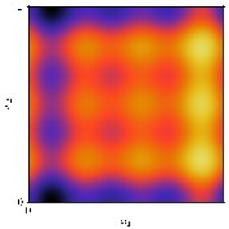
() $u(x_{1},x_{2})$

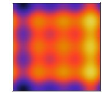
(a) $\delta c=(0,0)$

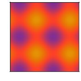
(b) $\delta c=(1/2,1/2)$

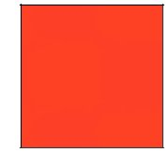
(c) $\delta c=(1/e,1/\pi)$

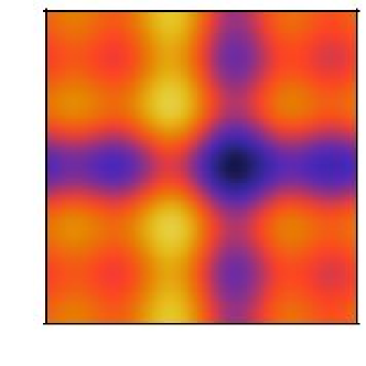
(d) $\int_{0}^{\infty}(c-c^{\prime}(s))\,ds=(1/2,1/2)$

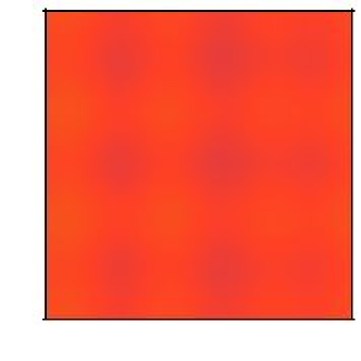
(e) $\int_{0}^{t}\left(c-c^{\prime}(s;\omega^{\prime})\right)\,ds=W(t)$

Figure 1: Figure 1() is the true initial condition. Figures 1(a) – 1(e) show the desired empirical mean of the smoothing $\mathbb{P}(v_{0}|Y_{n}=Y_{n}^{\prime})$ for $\delta c=(0,0),\delta c=(1/2,1/2),\delta c\in\mathbb{R}\setminus\mathbb{Q}\times\mathbb{R}\setminus\mathbb{Q},\int_{0}^{\infty}\delta c\,dt=(1/2,1/2)$ and $\delta c=\dot{W}$ respectively.

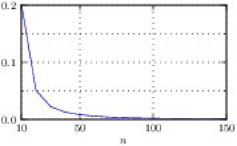
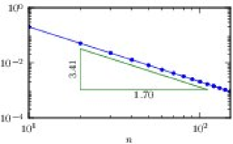
Figure 2: Plot 2 shows $\|\mathbb{E}(v_{n}|c,Y_{n}=Y_{n}^{\prime})-v^{\prime}_{n}\|^{2}_{L^{2}(\mathbb{T}^{2})}$ as a function of $n$, when $\int_{0}^{\infty}\delta c(s)\,ds=(1/2,1/2)$. Its $\log$-$\log$ plot, along with a least squares fit, is depicted in Plot 2, demonstrating quadratic convergence.

5.3 Sampling the wave velocity and initial condition

The objective of this subsection is to show that the problems caused by model error in the form of a constant shift to the wave velocity can be overcome by sampling $c$ and $v_{0}$. We generate data from (14), (15) with $c^{\prime}=c$ given by (35) and initial condition (36). We assume that neither the wave velocity nor the initial condition are known to us, and we attempt to recover them from given data.

The desired conditional distribution is multimodal with respect to $c$ – recall that it is non-Gaussian – and care is required to seed the chain close to the desired value in order to avoid metastability. Although the algorithm does not have access to the true signal $v^{\prime}_{n},$ we do have noisy observations of it: $y^{\prime}_{n}$. Thus it is natural to choose as initial $c=c^{*}$ for the Markov chain the value which minimizes

$$\sum_{j=1}^{n-1}\left\|\log\left(\frac{(v^{\prime}_{j+1},\phi_{k})}{(v^{\prime}_{j},\phi_{k})}\right)-2\pi ik\cdot c\Delta t\right\|^{2}.$$ (37)

Because of the observational noise this estimate is more accurate for small values of $k$ and we choose $k=(1,0)$ to estimate $c_{1}$ and $k=(0,1)$ to estimate $c_{2}$.

Figure 3 shows the marginal distribution for $c$ computed with four different values of the data size $n$, in all cases with the Markov chain seeded as in (37). The results show that the marginal wave velocity distribution $\mathbb{P}(c|Y_{n})$ converges to a Dirac on the true value as the amount of data is increased. Although not shown here, the initial condition is also converging to a Dirac on the true value (35) in this limit.

We round-off this subsection by mentioning related published literature. First we mention that, in a setting similar to ours, a scheme to approximate the true wave velocity is proposed which uses parameter estimation within 3D Var for the linear advection equation with constant velocity [9], and its hybrid with the EnKF for the non-constant velocity case [10]. These methodologies deal with the problem entirely in finite dimensions but are not limited to the linear dynamics. Secondly we note that, although a constant wave velocity parameter in the linear advection equation is a useful physical idealization in some cases, it is a very rigid assumption, making the data assimilation problem with respect to this parameter quite hard; this is manifest in the large number of samples required to estimate this constant parameter. A notable, and desirable, direction in which to extend this work numerically is to consider the time-dependent wave velocity as presented in Theorems 4.1–4.3. For efficient filtering techniques to estimate time-dependent parameters, the reader is directed to [39, 40, 41, 42].

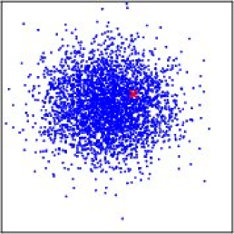
(a) $n=10$

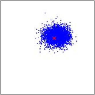
(b) $n=50$

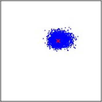
(c) $n=100$

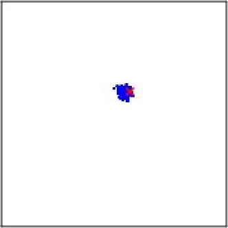
(d) $n=1000$

Figure 3: The marginal distribution of $\mathbb{P}(c,v_{0}|Y_{n})$ with respect to $c$ are depicted on the square $1.4\times 10^{-4}$ by $\times 10^{-4}$. The red cross marks the true wave velocity $c=(-0.5,-1.0)$.

6 Conclusions

In this paper, we study an infinite dimensional state estimation problem in the presence of model error. For the statistical model of advection equation on a torus, with noisily observed functions in discrete time, the large data limit of the filter and the smoother both recover the truth in the perfect model scenario. If the actual wave velocity differs from the true wave velocity in a time-integrable fashion then the filter recovers the truth, but the smoother is in error by a constant phase shift, determined by the integral of the difference in wave velocities. When the difference in wave velocities is constant neither filtering nor smoothing recovers the truth in the large data limit. And when the difference in wave velocities is a fluctuating random field, however small, neither filtering nor smoothing recovers the truth in the large data limit.

In this paper we consider the dynamics as a hard constraint, and do not allow for the addition of mean zero Gaussian noise to the time evolution of the state. Adding such noise to the model is sometimes known as a weak constraint approach in the data assimilation community and the relative merits of hard and weak constraint approaches are widely debated; see [4, 43] for discussion and references. New techniques of analysis would be required to study the weakly constrained problem, because the inverse covariance does not evolve linearly as it does for the hard constraint problem we study here. We leave this for future study.

There are a number of other ways in which the analysis in this paper could be generalized, in order to obtain a deeper understanding of filtering methods for high dimensional systems. These include: (i) the study of dissipative model dynamics; (ii) the study of nonlinear wave propagation problems; (iii) the study of Lagrangian rather than Eulerian data. Many other generalizations are also possible. For nonlinear systems, the key computational challenge is to find filters which can be justified, either numerically or analytically, and which are computationally feasible to implement. There is already significant activity in this direction, and studying the effect of model/data mismatch will form an important part of the evaluation of these methods.

Appendix A Basic Theorems on Gaussian Measures

Suppose the probability measure $\mu$ is defined on the Hilbert space $\mathcal{H}$. A function $m\in\mathcal{H}$ is called the mean of $\mu$ if, for all $\ell$ in the dual space of linear functionals on $\mathcal{H}$,

$$\ell(m)=\int_{\mathcal{H}}\ell(x)\mu(dx),$$

and a linear operator $\mathcal{C}$ is called the covariance operator if for all $k,\ell$ in the dual space of $\mathcal{H}$,

$$k\left(\mathcal{C}\ell\right)=\int_{\mathcal{H}}k(x-m)\ell(x-m)\mu(dx).$$

In particular, a measure $\mu$ is called Gaussian if $\mu\circ\ell^{-1}=\mathcal{N}\left(m_{\ell},\sigma_{\ell}^{2}\right)$ for some $m_{\ell},\sigma_{\ell}\in\mathbb{R}$. Since the mean and covariance operator completely determine a Gaussian measure, we denote a Gaussian measure with mean $m$ and covariance operator $\mathcal{C}$ by $\mathcal{N}(m,\mathcal{C})$.

The following lemmas, all of which can be found in [29], summarize the properties of Gaussian measures which we require for this paper.

Lemma A.1.

If $\mathcal{N}(0,\mathcal{C})$ is a Gaussian measure on a Hilbert space $\mathcal{H}$, then $\mathcal{C}$ is a self-adjoint, positive semi-definite nuclear operator on $\mathcal{H}$. Conversely, if $m\in\mathcal{H}$ and $\mathcal{C}$ is a self-adjoint, positive semi-definite, nuclear operator on $\mathcal{H}$, then there is a Gaussian measure $\mu=\mathcal{N}(m,\mathcal{C})$ on $\mathcal{H}$.

Lemma A.2.

Let $\mathcal{H}=\mathcal{H}_{1}\oplus\mathcal{H}_{2}$ be a separable Hilbert space with projections $\Pi_{i}:\mathcal{H}\to\mathcal{H}_{i},i=1,2$. For an $\mathcal{H}$-valued Gaussian random variable $(x_{1},x_{2})$ with mean $m=(m_{1},m_{2})$ and positive-definite covariance operator $\mathcal{C}$, denote $C_{ij}=\Pi_{i}\mathcal{C}\Pi_{j}^{*}$. Then the conditional distribution of $x_{1}$ given $x_{2}$ is Gaussian with mean

$$m_{1|2}=m_{1}-{C}_{12}{C}_{22}^{-1}(m_{2}-x_{2}),$$

and covariance operator

$$\mathcal{C}_{1|2}={C}_{11}-{C}_{12}{C}_{22}^{-1}{C}_{21}.$$

Lemma A.3.

(Feldman-Hajek) Two Gaussian measures $\mu_{i}=\mathcal{N}(m_{i},\mathcal{C}_{i})$, $i=1,2$, on a Hilbert space $\mathcal{H}$ are either singular or equivalent. They are equivalent if and only if the following three conditions hold:
(i) $\mbox{Im}\left(\mathcal{C}_{1}^{\frac{1}{2}}\right)=\mbox{Im}\left(\mathcal{C}_{2}^{\frac{1}{2}}\right):=E$;
(ii) $m_{1}-m_{2}\in E$;
(iii) the operator $T:=\left(\mathcal{C}_{1}^{-\frac{1}{2}}\mathcal{C}_{2}^{\frac{1}{2}}\right)\left(\mathcal{C}_{1}^{-\frac{1}{2}}\mathcal{C}_{2}^{\frac{1}{2}}\right)^{*}-I$ is Hilbert-Schmidt in $\bar{E}$.

Lemma A.4.

For any two positive-definite, self-adjoint operators $\mathcal{C}_{i}$, $i=1,2$, on a Hilbert space $\mathcal{H}$, the condition $\mbox{Im}\left(\mathcal{C}_{1}^{\frac{1}{2}}\right)\subseteq\mbox{Im}\left(\mathcal{C}_{2}^{\frac{1}{2}}\right)$ holds if and only if there exists a constant $K>0$ such that

$$\left(h,\mathcal{C}_{1}h\right)\leq K\left(h,\mathcal{C}_{2}h\right),\quad\forall h\in\mathcal{H}$$

where $(\cdot,\cdot)$ denotes the inner product on $\mathcal{H}$.

Lemma A.5.

For Gaussian $X$ on a Hilbert space $\mathcal{H}$ with norm $\left\|\cdot\right\|$ and for any integer $n$, there is constant $C_{n}\geq 0$ such that $\mathbb{E}(\left\|X\right\|^{2n})\leq C_{n}\left(\mathbb{E}\left(\left\|X\right\|^{2}\right)\right)^{n}$.

Appendix B Proof of Limit Theorems

In this Appendix, we will prove the Limit Theorems 3.2, 3.7, 4.1, where $\mathcal{L}=\mathcal{L}^{\prime}$, $\mathcal{L}\neq\mathcal{L}^{\prime}$, $\mathcal{L}(t)\neq\mathcal{L}^{\prime}(t)$, and Theorem 4.3 where $\mathcal{L}(t)\neq\mathcal{L}^{\prime}(t;\omega^{\prime})$, respectively. In all cases, we use the notations $e^{-t\mathcal{L}}$ and $e^{-t\mathcal{L}^{\prime}}$ to denote the forward solution operators through $t$ time units (from time zero in the non-autonomous case). We denote by ${M}$ the putative limit for $m^{\prime}_{n}$. The identity

$$\left(nI+\Gamma\mathcal{C}_{0}^{-1}\right)(m^{\prime}_{n}-{M}) =\Gamma\mathcal{C}_{0}^{-1}\left(m_{0}-{M}\right)+\sum_{l=0}^{n-1}e^{t_{l+1}\mathcal{L}}\eta^{\prime}_{l+1}$$ (38)

$$\quad+\sum_{l=0}^{n-1}\left(e^{t_{l+1}\left(\mathcal{L}-\mathcal{L}^{\prime}\right)}u-{M}\right),$$

obtained from Equation (16), will be used to show $m^{\prime}_{n}\to{M}$ . In Equation (38), we will choose $M$ so that the contribution of the last term is asymptotically negligible. Define the Fourier representations

$$\mathbf{e}_{n} \equiv m^{\prime}_{n}-{M}=\sum_{k\in\mathbb{K}}\hat{\mathbf{e}}_{n}(k)\phi_{k},$$

$$\mathbf{\xi}_{l} \equiv e^{t_{l+1}\left(\mathcal{L}-\mathcal{L}^{\prime}\right)}u-{M}=\sum_{k\in\mathbb{K}}\hat{\mathbf{\xi}}_{l}(k)\phi_{k}.$$

Then $M$ will be any one of $u$, $\mathcal{F}_{(p,q)}u$, $\langle u\rangle$ and $u_{\alpha}.$ Hence there is $C_{1}$ independent of $k,l$ such that $\hat{\mathbf{\xi}}_{l}(0)=0$ and $\mathbb{E}|\hat{\mathbf{\xi}}_{l}(k)|\leq C_{1}|\left(u,\phi_{k}\right)|$ with $C_{1}<\infty$ (the expectation here is trivial except in the case of random ${\mathcal{L}}^{\prime}$). Using Equation (19), these Fourier coefficients satisfy the relation

$$\left(n+\frac{\gamma_{k}}{\lambda_{k}}\right)\hat{\mathbf{e}}_{n}(k) =\frac{\gamma_{k}}{\lambda_{k}}\hat{\mathbf{e}}_{0}(k)+\sqrt{\gamma^{\prime}_{k}}\sum_{l=0}^{n-1}(\mathbf{g}_{k}^{\prime})^{l+1}+\sum_{l=0}^{n-1}\hat{\mathbf{\xi}}_{l}(k),\quad k\in\mathbb{K}.$$

In order to prove $m^{\prime}_{n}\to{M}$ in $L^{2}(\Omega^{\prime};H^{s}(\mathbf{T}^{2}))$, we use the monotone convergence theorem to obtain the following inequalities,

$$n^{\delta}\left\|\mathbf{e}_{n}\right\|^{2}_{L^{2}(\Omega^{\prime};H^{s}(\mathbf{T}^{2}))} =n^{\delta}\mathbb{E}\left\|\mathbf{e}_{n}\right\|^{2}_{H^{s}(\mathbf{T}^{2})}$$ (39)

$$=\sum_{k\in\mathbb{K}^{+}}|k|^{2s}n^{\delta}\mathbb{E}|\hat{\mathbf{e}}_{n}(k)|^{2}+n^{\delta}\mathbb{E}|\hat{\mathbf{e}}_{n}(0)|^{2}$$

$$=\sum_{k\in\mathbb{K}^{+}}|k|^{2s}\frac{n^{\delta}}{\left(n+{\gamma_{k}}/{\lambda_{k}}\right)^{2}}\Bigg{[}\left(\frac{\gamma_{k}}{\lambda_{k}}\right)^{2}|\hat{\mathbf{e}}_{0}(k)|^{2}+\gamma_{k}^{\prime}n$$

$$\quad+2\mbox{Re}\left\{\frac{\gamma_{k}}{\lambda_{k}}\bar{\hat{\mathbf{e}}}_{0}(k)\mathbb{E}\left(\sum_{l=0}^{n-1}\hat{\mathbf{\xi}}_{l}(k)\right)\right\}+\mathbb{E}\left|\sum_{l=0}^{n-1}\hat{\mathbf{\xi}}_{l}(k)\right|^{2}\Bigg{]}$$

$$\quad+\frac{n^{\delta}}{(n+{\gamma_{0}}/{\lambda_{0}})^{2}}\left[\left(\frac{\gamma_{0}}{\lambda_{0}}\right)^{2}|\hat{\mathbf{e}}_{0}(0)|^{2}+\gamma_{0}^{\prime}n\right]$$

$$\leq\sum_{k\in\mathbb{K}^{+}}|k|^{2s}{n^{\delta-2}}\Bigg{[}\left(\frac{\gamma_{k}}{\lambda_{k}}\right)^{2}|\hat{\mathbf{e}}_{0}(k)|^{2}$$

$$\quad+\gamma_{k}^{\prime}n+2C_{1}\frac{\gamma_{k}}{\lambda_{k}}|\hat{\mathbf{e}}_{0}(k)||(u,\phi_{k})|n+\mathbb{E}\left|\sum_{l=0}^{n-1}\hat{\mathbf{\xi}}_{l}(k)\right|^{2}\Bigg{]}$$

$$\quad+n^{\delta-2}\left[\left(\frac{\gamma_{0}}{\lambda_{0}}\right)^{2}|\hat{\mathbf{e}}_{0}(0)|^{2}+\gamma_{0}^{\prime}n\right]$$

$$\leq\sum_{k\in\mathbb{K}^{+}}|k|^{2s}{n^{\delta-2}}\Bigg{[}\left(\frac{\gamma_{k}}{\lambda_{k}}\right)^{2}|\hat{\mathbf{e}}_{0}(k)|^{2}+\gamma_{k}^{\prime}n$$

$$\quad+C_{1}\left(\left(\frac{\gamma_{k}}{\lambda_{k}}\right)^{2}|\hat{\mathbf{e}}_{0}(k)|^{2}+|(u,\phi_{k})|^{2}\right)n+\mathbb{E}\left|\sum_{l=0}^{n-1}\hat{\mathbf{\xi}}_{l}(k)\right|^{2}\Bigg{]}$$

$$\quad+n^{\delta-2}\left[\left(\frac{\gamma_{0}}{\lambda_{0}}\right)^{2}|\hat{\mathbf{e}}_{0}(0)|^{2}+\gamma_{0}^{\prime}n\right]$$

$$\leq\left(C\left\|m_{0}-{M}\right\|_{H^{s+\kappa}(\mathbf{T}^{2})}\right)n^{\delta-2}+\left(\sum_{k\in\mathbb{K}}|k|^{2s}\gamma_{k}^{\prime}\right)n^{\delta-1}$$

$$\quad+\left(C_{1}\left\|u\right\|_{H^{s}(\mathbf{T}^{2})}\right)n^{\delta-1}+\left(\sum_{k\in\mathbb{K}^{+}}|k|^{2s}n^{\delta-2}\mathbb{E}\left|\sum_{l=0}^{n-1}\hat{\mathbf{\xi}}_{l}(k)\right|^{2}\right)$$

$$\leq C\left(\left\|m_{0}\right\|_{H^{s+\kappa}(\mathbf{T}^{2})}+\left\|u\right\|_{H^{s+\kappa}(\mathbf{T}^{2})}\right)n^{\delta-2}$$

$$\quad+\left(\sum_{k\in\mathbb{K}}|k|^{2s}\gamma_{k}^{\prime}+C_{1}\left\|u\right\|_{H^{s}(\mathbf{T}^{2})}\right)n^{\delta-1}$$

$$\quad+\left(\sum_{k\in\mathbb{K}}|k|^{2s}n^{\delta-2}\mathbb{E}\left|\sum_{l=0}^{n-1}\hat{\mathbf{\xi}}_{l}(k)\right|^{2}\right),$$

and here the first two terms in the last equation can be controlled by Assumptions 3.1. In order to find $\delta\in[0,1]$ such that this equation is $O(1)$ or $o(1)$,

$$\sum_{k\in\mathbb{K}}|k|^{2s}n^{\delta-2}\mathbb{E}\left|\sum_{l=0}^{n-1}\hat{\mathbf{\xi}}_{l}(k)\right|^{2}$$ (40)

is the key term. This term arises from the model error, i.e., the discrepancy between the operator $\mathcal{L}$ used in the statistical model and the operator $\mathcal{L}^{\prime}$ which generates the data. We analyze it, in various cases, in the subsections which follow.

In order to prove $m^{\prime}_{n}\to{M}$ in $H^{s}(\mathbf{T}^{2}),\;\Omega^{\prime}-a.s.$, suppose we have

$$\frac{1}{n}\sum_{l=0}^{n-1}\hat{\mathbf{\xi}}_{l}(k)\to 0\quad\Omega^{\prime}-a.s.,$$ (41)

for each $k\in\mathbb{K}$. We then use the strong law of large numbers to obtain the following inequalities, which holds $\Omega^{\prime}-a.s.$,

$$\left\|\mathbf{e}_{n}\right\|^{2}_{H^{s}(\mathbf{T}^{2})} =\sum_{k\in\mathbb{K}^{+}}|k|^{2s}|\hat{\mathbf{e}}_{n}(k)|^{2}+|\hat{\mathbf{e}}_{n}(0)|^{2}$$ (42)

$$=\sum_{k\in\mathbb{K}^{+}}|k|^{2s}\left|\frac{\left({\gamma_{k}}/{\lambda_{k}}\right)\hat{\mathbf{e}}_{0}(k)+\sqrt{\gamma^{\prime}_{k}}\sum_{l=0}^{n-1}(\mathbf{g}_{k}^{\prime})^{l+1}+\sum_{l=0}^{n-1}\hat{\mathbf{\xi}}_{l}(k)}{n+{\gamma_{k}}/{\lambda_{k}}}\right|^{2}$$

$$\quad+\left|\frac{\left({\gamma_{0}}/{\lambda_{0}}\right)\hat{\mathbf{e}}_{0}(0)+\sqrt{\gamma^{\prime}_{0}}\sum_{l=0}^{n-1}(\mathbf{g}_{0}^{\prime})^{l+1}}{n+{\gamma_{0}}/{\lambda_{0}}}\right|^{2}$$

$$\leq C\sum_{k\in\mathbb{K}}(1+|k|^{2s})\Bigg{(}\left|\frac{\left({\gamma_{k}}/{\lambda_{k}}\right)\hat{\mathbf{e}}_{0}(k)}{n}\right|^{2}+\left|\frac{\sqrt{\gamma^{\prime}_{k}}\sum_{l=0}^{n-1}(\mathbf{g}_{k}^{\prime})^{l+1}}{n}\right|^{2}$$

$$\quad+\left|\frac{\sum_{l=0}^{n-1}\hat{\mathbf{\xi}}_{l}(k)}{n}\right|^{2}\Bigg{)}$$

$$\leq C\sum_{k\in\mathbb{K}}(1+|k|^{2s})\left(|k|^{2\kappa}|\hat{\mathbf{e}}_{0}(k)|^{2}+\gamma_{k}^{\prime}+|(u,\phi_{k})|^{2}\right)$$

$$\leq C\left(\left\|m_{0}\right\|_{H^{s+\kappa}(\mathbf{T}^{2})}+\left\|u\right\|_{H^{s+\kappa}(\mathbf{T}^{2})}+\sum_{k\in\mathbb{K}}|k|^{2s}\gamma_{k}^{\prime}+\left\|u\right\|_{H^{s}(\mathbf{T}^{2})}\right).$$

Therefore, using Weierstrass M-test, we have $\left\|\mathbf{e}_{n}\right\|^{2}_{H^{s}(\mathbf{T}^{2})}\to 0,\;\Omega^{\prime}-a.s.$, once Equation (41) is satisfied.

B.1 Proof of Theorem 3.2

This proof is given directly after the theorem statement. For completeness we note that Equation (17a) follows from Equation (39) with $\delta=1$. Once it has been established that

$$\left\|\cdot\right\|_{L^{2}(\Omega^{\prime};H^{s}(\mathbf{T}^{2}))}=O\left(n^{-\delta/2}\right),$$

then the proof that

$$\left\|\cdot\right\|_{H^{s}(\mathbf{T}^{2})}=o\left(n^{-\theta}\right)\quad\Omega^{\prime}-a.s.,$$

for any $\theta<\delta/2$ follows from a Borel-Cantelli argument as shown in the proof of Theorem 3.2. We will not repeat this argument for the proofs of Theorems 3.7, 4.1 and 4.3.

B.2 Proof of Theorem 3.7

B.2.1

When $\mathcal{L}\neq\mathcal{L}^{\prime}$ and $\Delta t\,\delta c=(p^{\prime}/p,q^{\prime}/q)$, choose ${M}=\mathcal{F}_{(p,q)}u$ then

$$\hat{\mathbf{\xi}}_{l}(k) =e^{2\pi i(k\cdot\delta c)t_{l+1}}(u,\phi_{k})-\delta^{k}_{(p,q)}(u,\phi_{k})$$

$$=\left(1-\delta^{k}_{(p,q)}\right)e^{2\pi i(k\cdot\delta c)t_{l+1}}(u,\phi_{k}),$$

where $\delta^{k}_{(p,q)}$ is $1$ if $k_{1}$ and $k_{2}$ for $k=(k_{1},k_{2})$ are multiples of $p$ and $q$ respectively, and $0$ otherwise. Using

$$\left|\sum_{l=0}^{n-1}\hat{\mathbf{\xi}}_{l}(k)\right|^{2} =\left(1-\delta^{k}_{(p,q)}\right)^{2}\left|\sum_{l=0}^{n-1}e^{2\pi i(k\cdot\delta c)t_{l+1}}\right|^{2}|(u,\phi_{k})|^{2}$$

$$=\left(1-\delta^{k}_{(p,q)}\right)\left[\frac{\sin(n\pi(k\cdot\delta c)\Delta t)}{\sin(\pi(k\cdot\delta c)\Delta t)}\right]^{2}|(u,\phi_{k})|^{2}$$

$$\leq\left[\sin^{2}\left(\pi\left(\frac{1}{p}+\frac{1}{q}\right)\right)\right]^{-1}|(u,\phi_{k})|^{2},$$

the quantity in Equation (40) becomes

$$\left(\left[\sin^{2}\left(\pi\left(\frac{1}{p}+\frac{1}{q}\right)\right)\right]^{-1}\left\|u\right\|_{H^{s}(\mathbf{T}^{2})}\right)n^{\delta-2},$$

so that from Equation (39)

$$n\left\|\mathbf{e}_{n}\right\|^{2}_{L^{2}(\Omega^{\prime};H^{s}(\mathbf{T}^{2}))}=O(1).$$

B.2.2

When $\mathcal{L}\neq\mathcal{L}^{\prime}$ and $\Delta t\,\delta c\in\mathbb{R}\backslash\mathbb{Q}\times\mathbb{R}\backslash\mathbb{Q}$, choose ${M}=\langle u\rangle$ then

$$\hat{\mathbf{\xi}}_{l}(k)=e^{2\pi i(k\cdot\delta c)t_{l+1}}(u,\phi_{k}),$$

for $k\in\mathbb{K}^{+}$. It is immediate that

$$\left\|\mathbf{e}_{n}\right\|_{H^{s}(\mathbf{T}^{2})}=o(1)\quad\Omega^{\prime}-a.s.,$$

since

$$\frac{1}{n}\sum_{l=0}^{n-1}e^{2\pi i(k\cdot\delta c)t_{l+1}}=o(1),$$

as $n\to\infty$, by ergodicity  [33] and Equation (41). Furthermore, when $\delta=0$, the quantity in Equation (40) is bounded by

$$\sum_{k\in\mathbb{K}}|k|^{2s}\left|\frac{1}{n}\sum_{l=0}^{n-1}e^{2\pi i(k\cdot\delta c)t_{l+1}}\right|^{2}|(u,\phi_{k})|^{2}\leq C\|u\|_{H^{s}(\mathbf{T}^{2})},$$

and Weierstrass M-test can be used to show

$$\left\|\mathbf{e}_{n}\right\|^{2}_{L^{2}(\Omega^{\prime};H^{s}(\mathbf{T}^{2}))}=o(1).$$

B.3 Proof of Theorem 4.1

When $\mathcal{L}(t)\neq\mathcal{L}^{\prime}(t)$ and $\int^{t}_{0}\delta c(s)\,ds=\alpha+O(t^{-\beta})$, choose ${M}=u_{\alpha}$ then

$$\hat{\mathbf{\xi}}_{l}(k)=\left(e^{2\pi ik\cdot\left(\int^{t_{l+1}}_{0}\delta c(s)\,ds\right)}-e^{2\pi ik\cdot\alpha}\right)(u,\phi_{k}),$$

and we obtain

$$\left|\sum_{l=0}^{n-1}\hat{\mathbf{\xi}}_{l}(k)\right|^{2}=\left|\sum_{l=0}^{n-1}\left(e^{2\pi ik\cdot\left(\int^{t_{l+1}}_{0}\delta c(s)\,ds-\alpha\right)}-1\right)\right|^{2}|(u,\phi_{k})|^{2}.$$

Now utilizing that

$$\left|\sum_{l=0}^{n-1}\left(e^{ix_{l}}-1\right)\right|\leq C\sum_{l=0}^{n-1}|x_{l}|\leq C_{2}n^{1-\beta},$$

when $x_{l}=O\left(l^{-\beta}\right)$ and for $\beta\in(0,1/2]$, Equation (39) gives

$$n^{\delta}\left\|\mathbf{e}_{n}\right\|^{2}_{L^{2}(\Omega^{\prime};H^{s}(\mathbf{T}^{2}))} \leq C\left(\left\|m_{0}\right\|_{H^{s+\kappa}(\mathbf{T}^{2})}+\left\|u\right\|_{H^{s+\kappa}(\mathbf{T}^{2})}\right)n^{\delta-2}$$

$$\quad+\left(\sum_{k\in\mathbb{K}}|k|^{2s}\gamma_{k}^{\prime}+C_{1}\left\|u\right\|_{H^{s}(\mathbf{T}^{2})}\right)n^{\delta-1}$$

$$\quad+\left(C_{2}\left\|u\right\|^{2}_{H^{s}(\mathbf{T}^{2})}\right)n^{\delta-2\beta}=O(1),$$

for $\delta=1\wedge 2\beta$.

B.4 Proof of Theorem 4.3

When $\mathcal{L}(t)\neq\mathcal{L}^{\prime}(t;\omega^{\prime})$ and $\int^{t}_{0}c^{\prime}(s;\omega^{\prime})\,ds=\int^{t}_{0}c(s)\,ds-\varepsilon{W}(t)$, choose ${M}=\langle u\rangle$ then we obtain

$${\mathbf{\xi}}_{l}=u\left(\cdot+\varepsilon W(t_{l+1})\right)-\langle u\rangle,$$

and

$$\hat{\mathbf{\xi}}_{l}(k)=e^{2\pi ik\cdot\varepsilon W(t_{l+1})}(u,\phi_{k}),$$

for $k\in\mathbb{K}^{+}$. Using

$$\mathbb{E}\left|\sum_{l=0}^{n-1}\hat{\mathbf{\xi}}_{l}(k)\right|^{2} =\mathbb{E}\left(\sum_{l=0}^{n-1}\sum_{l^{\prime}=0}^{n-1}e^{2\pi ik\cdot\varepsilon\left(W(t_{l+1})-W(t_{l^{\prime}+1})\right)}|(u,\phi_{k})|^{2}\right)$$

$$=\sum_{l=0}^{n-1}\sum_{l^{\prime}=0}^{n-1}e^{-2\pi^{2}\varepsilon^{2}|k|^{2}\Delta t|l-l^{\prime}|}|(u,\phi_{k})|^{2}$$

$$=\left(n+2\sum_{l=1}^{n-1}\sum_{l^{\prime}=0}^{n-1}e^{-2\pi^{2}\varepsilon^{2}|k|^{2}\Delta t|l-l^{\prime}|}|\right)(u,\phi_{k})|^{2}$$

$$=\left[n+\frac{2}{e^{2\pi^{2}\varepsilon^{2}|k|^{2}\Delta t}-1}\left(\frac{e^{-2\pi^{2}\varepsilon^{2}|k|^{2}\Delta t(n-1)}-1}{e^{2\pi^{2}\varepsilon^{2}|k|^{2}\Delta t}-1}+n-1\right)\right]|(u,\phi_{k})|^{2}$$

$$\leq\left[n+\frac{2}{e^{2\pi^{2}\varepsilon^{2}\Delta t}-1}n\right]|(u,\phi_{k})|^{2}=\left(\frac{e^{2\pi^{2}\varepsilon^{2}\Delta t}+1}{e^{2\pi^{2}\varepsilon^{2}\Delta t}-1}\right)n|(u,\phi_{k})|^{2},$$

we get

$$\sum_{k\in\mathbb{K}^{+}}|k|^{2s}n^{\delta-2}\mathbb{E}\left|\sum_{l=0}^{n-1}\hat{\mathbf{\xi}}_{l}(k)\right|^{2}\leq\left(\frac{e^{2\pi^{2}\varepsilon^{2}\Delta t}+1}{e^{2\pi^{2}\varepsilon^{2}\Delta t}-1}\right)\left\|u\right\|^{2}_{H^{s}(\mathbf{T}^{2})}n^{\delta-1}=O(1),$$

for $\delta=1$.

References

References

- [1] Anderson B, Moore J and Barratt J 1979
- [2] Doucet A, De Freitas N and Gordon N 2001 Sequential Monte Carlo methods in practice (Springer Verlag) ISBN 0387951466
- [3] Kalman R et al. 1960 Journal of basic Engineering 82 35–45
- [4] Bennett A 2002 Inverse modeling of the ocean and atmosphere (Cambridge Univ Pr) ISBN 0521813735
- [5] Evensen G 1994 Journal of geophysical research 99 10143 ISSN 0148-0227
- [6] Kalnay E 2003 Atmospheric modeling, data assimilation, and predictability (Cambridge Univ Pr) ISBN 0521796296
- [7] van Leeuwen P 2009
- [8] Majda A and Grote M 2007 Proceedings of the National Academy of Sciences 104 1124
- [9] Smith P, Dance S, Baines M, Nichols N and Scott T 2009 Ocean Dynamics 59 697–708 ISSN 1616-7341
- [10] Smith P, Dance S and Nichols N 2010
- [11] Griffith A and Nichols N 2001 J. of Flow, Turbulence and Combustion 65 469–488
- [12] Evensen G 2009 Data assimilation: The ensemble Kalman filter (Springer Verlag) ISBN 3642037100
- [13] Evensen G v L P J 1996 Monthly Weather Review 124 85–96
- [14] Snyder C, Bengtsson T, Bickel P and Anderson J 2008 Monthly Weather Review 136 4629–4640 ISSN 1520-0493
- [15] Bengtsson T, Bickel P and Li B 2008 Probability and Statistics: Essays in Honor of David A. Freedman 2 316–334
- [16] Bickel P, Li B and Bengtsson T 2008 IMS Collections: Pushing the Limits of Contemporary Statistics: Contributions in Honor of Jayanta K. Ghosh 3 318–329
- [17] Chorin A and Krause P 2004 Proceedings of the National Academy of Sciences of the United States of America 101 15013
- [18] Chorin A and Tu X 2009 Proceedings of the National Academy of Sciences 106 17249
- [19] Chorin A and Tu X 2009 Arxiv preprint arXiv:0910.3241
- [20] Harlim J and Majda A 2008 Nonlinearity 21 1281
- [21] Castronovo E, Harlim J and Majda A 2008 Journal of Computational Physics 227 3678–3714 ISSN 0021-9991
- [22] Majda A, Harlim J and Gershgorin B 2010 Discrete and Continuous Dynamical Systems 27 441–486
- [23] Jean-Pierre F and Simoni A 2010 IDEI Working Papers
- [24] Neubauer A and Pikkarainen H 2008 Journal of Inverse and Ill-posed Problems 16 601–613 ISSN 0928-0219
- [25] van der Vaart A W and van Zanten J H 2008 Annals of Statistics 36 1435–1463
- [26] Pikkarainen H 2006 Inverse Problems 22 365
- [27] Smith P, Dance S, Baines M, Nichols N and Scott T 2009 Ocean Dynamics 59 697–708 ISSN 1616-7341
- [28] Cotter S, Dashti M, Robinson J and Stuart A 2009 Inverse Problems 25 115008
- [29] Da Prato G and Zabczyk J 1992 Stochastic equations in infinite dimensions (Cambridge Univ Pr) ISBN 0521385296
- [30] Varadhan S 2001 New York University Courant Institute of Mathematical Sciences, New York
- [31] Bogachev V 1998 Gaussian measures vol 62 (American Mathematical Society)
- [32] Kumar P and Varaiya P 1986 Stochastic systems: estimation, identification and adaptive control (Prentice-Hall, Inc.)
- [33] Breiman L 1968 Reading, Mass
- [34] Flandoli F, Gubinelli M and Priola E 2010 Inventiones Mathematicae 180 1–53 ISSN 0020-9910
- [35] Stuart A 2010 Acta Numerica 19 451–559 ISSN 1474-0508
- [36] Cotter SL D M and Robinson JC S A 2011 International Journal for Numerical Methods in Fluids
- [37] Geweke J and Tanizaki H 2001 Computational Statistics & Data Analysis 37 151–170 ISSN 0167-9473
- [38] Roberts G and Rosenthal J 2006 The Annals of Applied Probability 16 2123–2139 ISSN 1050-5164
- [39] Cohn S 1997 Journal of the Metereological Society of Japan 75 147–178
- [40] Dee D and Da Silva A 1998 Quarterly Journal of the Royal Meteorological Society 124 269–295
- [41] Baek S, Hunt B, Kalnay E, Ott E and Szunyogh I 2006 Tellus Series A 58 293–306
- [42] Gershgorin B, Harlim J and Majda A 2010 Journal of Computational Physics 229 1–31
- [43] Apte A, Jones C, Stuart A and Voss J 2008 International Journal for Numerical Methods in Fluids 56 1033–1046