Hamiltonian approach to Yang-Mills theory in Coulomb gauge - revisited^¶

Abstract

I briefly review results obtained within the variational Hamiltonian approach to Yang-Mills theory in Coulomb gauge and confront them with recent lattice data. The variational approach is extended to non-Gaussian wave functionals including three- and four-gluon kernels in the exponential of the vacuum wave functional and used to calculate the three-gluon vertex. A new functional renormalization group flow equation for Hamiltonian Yang–Mills theory in Coulomb gauge is solved for the gluon and ghost propagator under the assumption of ghost dominance. The results are compared to those obtained in the variational approach.

1 Introduction

In recent years there have been substantial efforts devoted to non-perturbative studies of continuum Yang–Mills theory. Among these are variational solutions of the Yang–Mills Schrödinger equation in Coulomb gauge (1; 2; 3). In this approach the energy density is minimized using Gaussian-type ansätze for the vacuum wave functional. In this talk I will first briefly review results obtained within the Tübingen approach (2) using a modified Gaussian wave functional. Then I will present a new approach to Hamiltonian quantum field theory, which allows to use non-Gaussian wave functionals in variational calculations (4). The approach is illustrated by using a wave functional with cubic and quartic gluonic terms in the exponential and applied to calculate the three-gluon vertex. Finally, I will discuss a new functional renormalization group (FRG) approach to the Hamiltonian formulation of Yang–Mills theory (5) and present results supporting the findings of the variational approach (2; 3).

2 Variational Approach

Instead of working with gauge invariant wave functionals, it is usually more convenient to fix the gauge. A particularly convenient choice of gauge is the Coulomb gauge $\bm{\nabla}\cdot\bm{A}=0$, which allows an explicit resolution of Gauss’ law, resulting in the gauge fixed Yang–Mills Hamiltonian (6)

$$H_{\textsc{ym}} =\frac{1}{2}\int d^{D}x\left(J^{-1}[\bm{A}]\,{\bm{\Pi}}J[\bm{A}]\,\bm{\Pi}+\bm{B}^{2}\right)+H_{c},$$ (1)

$$H_{c} =\frac{g^{2}}{2}\int d^{D}(x,x^{\prime})J^{-1}[\bm{A}]\rho^{a}(x)J[\bm{A}]F^{ab}(x,y)\rho^{b}(x),$$

where $\Pi^{a}(x)=\delta/i\delta A^{a}(x)$ is the canonical momentum (electric field) operator and

$$J[\bm{A}]=\mathrm{Det}(-\bm{D}\bm{\nabla})$$ (2)

is the Faddeev–Popov determinant. Furthermore

$$\rho^{a}(x)=-f^{abc}\bm{A}^{b}\bm{\Pi}^{c}$$ (3)

is the color charge of the gluons and

$$F^{ab}(x,y)=\langle x,a\rvert(-\bm{D}\bm{\nabla})^{-1}\,(-\bm{\nabla}^{2})\,(-\bm{D}\bm{\nabla})^{-1}\lvert y,b\rangle$$ (4)

is the so-called Coulomb kernel. In the presence of matter fields with color charge density $\rho^{a}_{m}(x)$, the gluon charge $\rho^{a}(x)$ in the Coulomb term is replaced by the total charge $\rho^{a}(x)+\rho^{a}_{m}(x)$ and the vacuum expectation value of $F^{ab}(x,y)$ acquires the meaning of the static non-Abelian Coulomb potential, see eq. (16) below.

The gauge fixed Hamiltonian eq. (1) is highly non-local due to the Coulomb kernel $F^{ab}(x,y)$, eq. (4), and due to the Faddeev–Popov determinant $J[\bm{A}]$, eq. (2). In addition, the latter also occurs in the functional integration measure of the scalar product of Coulomb gauge wave functionals

$$\langle\psi_{1}|O|\psi_{2}\rangle=\int DA\,J[\bm{A}]\,\psi^{*}_{1}[\bm{A}]\,O\,\psi_{2}[\bm{A}].$$ (5)

While the elimination of unphysical degrees of freedom via gauge fixing is often beneficial (and sometimes unavoidable) in practical calculations, the price to pay is the increased complexity of the gauge fixed Hamiltonian eq. (1). The non-trivial Faddeev–Popov determinant reflects the intrinsically non-linear structure of the space of gauge orbits and dominates the IR behavior of the theory. Once Coulomb gauge is implemented, any functional of the (transverse) gauge field is a physical state.

Treating the Hamiltonian (1) in the ordinary Rayleigh-Schrödinger perturbation theory one finds to leading order the usual one-loop $\beta$ function with $\beta_{0}=-\frac{11}{3}N_{c}$ (7). Our main interest lies, however, in the IR sector of the theory, which requires a non-perturbative treatment.

In ref. (2) the vacuum energy density was minimized using the following ansatz for the vacuum functional

$$\Psi[\bm{A}]=\frac{{\cal N}}{\sqrt{J[\bm{A}]}}\,\exp\left[-\frac{1}{2}\int\frac{d^{3}k}{(2\pi)^{3}}\omega(\bm{k})A_{i}^{a}(\bm{k})A_{i}^{a}(-\bm{k})\right].$$ (6)

For this wave functional the static gluon propagator is given by

$$\langle A^{a}_{i}(-\bm{k})A^{b}_{j}(\bm{q})\rangle=\delta^{ab}t_{ij}(\bm{k})(2\pi)^{3}\delta(\bm{k}-\bm{q})\frac{1}{2\omega(\bm{k})}\,,$$ (7)

so that $\omega(\bm{k})$ represents the (quasi-) gluon energy.

To the order considered in ref. (2), i.e., up to two loops in the energy (which corresponds to one loop in the associated Dyson–Schwinger equations), it was shown (8) that the Faddeev–Popov determinant, eq. (2), can be represented as

$$J[\bm{A}]=\exp\left[-\int d^{3}x\,d^{3}y\>A^{a}_{i}(x)\chi^{ab}_{ij}(x,y)A^{b}_{j}(y)\right],$$ (8)

where

$$\chi^{ab}_{ij}(x,y)=-\frac{1}{2}\left\langle\frac{\delta^{2}\ln J[\bm{A}]}{\delta A^{a}_{i}(x)\delta A^{b}_{j}(y)}\right\rangle=\delta^{ab}t_{ij}(x)\chi(x,y)$$ (9)

is the ghost loop and represents a measure of the curvature (2) of the Coulomb gauge fixed configuration space. Expressing the ghost Green’s function as

$$\langle(-D\bm{\nabla})^{-1}\rangle=\frac{d}{g(-\Delta)}\,,$$ (10)

where $d(\bm{k})$ is the ghost form factor, its Dyson–Schwinger equation reads to one-loop order

$$d^{-1}(\bm{k})=g^{-1}-I_{d}(\bm{k}),$$ (11)

$$I_{d}(\bm{k})=\frac{N_{c}}{2}\int\frac{d^{3}q}{(2\pi)^{2}}\,\left[1-(\hat{\bm{k}}\cdot\hat{\bm{q}})^{2}\right]\,\frac{d(\bm{q}-\bm{k})}{\omega(\bm{q})\,(\bm{q}-\bm{k})^{2}}\,.$$ (12)

The ghost form factor $d(\bm{k})$ measures the deviation from the QED case, where $d(\bm{k})=1$. Furthermore, $d^{-1}(\bm{k})$ represents the dielectric function of the Yang–Mills vacuum, and the so-called horizon condition

$$d^{-1}(0)=0$$ (13)

ensures that the Yang–Mills vacuum is a dual superconductor (9). Minimization of the vacuum energy $\langle H_{\textsc{ym}}\rangle$ with respect to the kernel $\omega(\bm{k})$ leads to the gap equation, which after renormalization reads (2), (10)

$$\omega^{2}(\bm{k})=\bm{k}^{2}+\chi^{2}(\bm{k})+c_{2}+\Delta I^{(2)}(\bm{k})+\\ +2\chi(\bm{k})\,[\Delta I^{(1)}(\bm{k})+c_{1}]\,,$$ (14)

where

$$\Delta I^{(n)}(\bm{k})={} I^{(n)}(\bm{k})-I^{(n)}(0),\qquad\overline{\omega}(\bm{k})\equiv\omega(\bm{k})-\chi(\bm{k}),$$

$$I^{(n)}(\bm{k})={} \frac{N_{c}}{4}\int\frac{d^{3}q}{(2\pi)^{3}}\left(1+(\hat{\bm{k}}\cdot\hat{\bm{q}})^{2}\right)V(\bm{q}-\bm{k})$$

$$\qquad\qquad\times\frac{\overline{\omega}^{n}(\bm{q})-\overline{\omega}^{n}(\bm{k})}{\omega(\bm{q})}\,,$$ (15)

and

$$V(\bm{k})\equiv g^{2}\,\langle F\rangle=\frac{d^{2}(\bm{k})}{\bm{k}^{2}}$$ (16)

is the non-Abelian Coulomb potential, where the approximation

$$\big{\langle}\,(-\bm{D}\bm{\nabla})^{-1}\cdot(-\bm{\nabla}^{2})\cdot(-\bm{D}\bm{\nabla})^{-1}\,\big{\rangle}\\ \qquad\qquad{}\approx\big{\langle}\,(-\bm{D}\bm{\nabla})^{-1}\,\big{\rangle}\cdot(-\bm{\nabla}^{2})\cdot\big{\langle}\,(-\bm{D}\bm{\nabla})^{-1}\,\big{\rangle}$$ (17)

has been used. In the gap equation (14), $c_{1}$ and $c_{2}$ are (finite) renormalization constants. For the critical solution, where one imposes the horizon condition (13), both $\omega(\bm{k})$ and $\chi(\bm{k})$ are infrared divergent, which implies that the transverse gluon propagator vanishes at $k\rightarrow 0$, while

$$\overline{\omega}(0)\equiv\lim_{k\rightarrow 0}(\omega(\bm{k})-\chi(\bm{k}))=c_{1}.$$ (18)

A perimeter law of the ’t Hooft loop requires $c_{1}=0$ and this value is also favored by the variational principle (10). Furthermore, for $c_{1}=0$ the IR limit of the wave functional (6) is

$$\psi[\bm{A}]={\cal N}\prod\limits_{\bm{k}}\psi(\bm{k}),\qquad\psi(\bm{k}=0)=1,$$ (19)

which is the exact vacuum wave functional in $1+1$ dimensions (11). The renormalization parameter $c_{2}$, on the other hand, has no influence on the IR or UV behavior of the solutions of the gap equation (14). Only the mid-momentum regime of $\omega(\bm{k})$ is weakly dependent on $c_{2}$ (2). Since we are mainly interested in the IR properties we will put $c_{2}=0$.

Figure 1: Gluon propagator obtained with a Gaussian (dashed line) and a non-Gaussian functional (straight line), compared to the lattice data from Ref. (12).

The coupled integral equations (11) and (14) can be solved analytically in the IR (for the critical solution satisfying the horizon condition (13)) using power law ansätze (2; 13)

$$\omega(\bm{k})\sim k^{-\alpha},\qquad d(\bm{k})\sim k^{-\beta}.$$ (20)

Under the assumption of a trivial scaling of the ghost-gluon vertex one finds that in $D$ space dimensions the IR exponents satisfy the sum rule

$$\alpha=2\beta+2-D.$$ (21)

This sum rule ensures that $\chi(\bm{k})$ has the same IR behavior as $\omega(\bm{k})$, cf. eq. (18). Furthermore, in $D=3$ one finds two solutions (13)

$$\beta\simeq 0.8\quad\text{and}\quad\beta=1.$$ (22)

The latter gives rise to a Coulomb potential (16) which is strictly linear at large distances. In $D=2$ only one solution $\beta=\frac{2}{5}$ is found, implying $\alpha=\frac{4}{5}$ and a Coulomb potential (16) rising as $V(r)\sim r^{4/5}$ (14). Furthermore in $D=2$ only the critical solution satisfying (13) exists (14). On the lattice, on the other hand, one finds $\alpha=1$ in $D=3$ and a linearly rising potential (15). In the UV-regime the coupled equations (11) and (14) can be solved perturbatively and one finds at large momenta $k\gg 1$ (2)

$$\omega(\bm{k})\sim k,\qquad d(\bm{k})\sim 1/\sqrt{\log(k)}.$$ (23)

The full numerical solutions of the above equations were given, for $D=3$ space dimensions, in refs. (2) and (3), where the critical solutions $\beta=0.8$ and $\beta=1$, respectively, were found, and for $D=2$ in ref. (14). One finds an inverse gluon propagator which in the UV behaves like the photon energy but diverges in the IR, signaling confinement in agreement with the IR analysis (20), (21), (22). Figures 1 and 2 show the resulting gluon energy $\omega(\bm{k})$ and non-Abelian Coulomb potential (16) for the solution $\beta=1$.

Figure 2: The numerical solution for the static non-Abelian Coulomb potential (3).

Their IR behavior is in agreement with the results of the IR analysis. The obtained propagator also compares favorably with the available lattice data (12). There are, however, deviations in the mid-momentum regime (and minor ones in the UV) which can be attributed to the missing gluon loop, which escapes the Gaussian wave functionals. These deviations are presumably irrelevant for the confinement properties, which are dominated by the ghost loop (which is fully included under the Gaussian ansatz), but are believed to be important for a correct description of spontaneous breaking of chiral symmetry (16).

3 Non-Gaussian wave functionals

In ref. (4) the variational approach to Yang–Mills theory in Coulomb gauge was extended to non-Gaussian wave functionals of the form

$$\lvert\psi[\bm{A}]\rvert^{2}=\exp(-S[\bm{A}]),$$ (24)

$$S[A]=\int\omega\bm{A}^{2}+\frac{1}{3!}\int\gamma_{3}\bm{A}^{3}+\frac{1}{4!}\int\gamma_{4}\bm{A}^{4},$$ (25)

where $\omega$, $\gamma_{3}$, $\gamma_{4}$ are variational kernels.

Representing the Faddeev–Popov determinant by a functional integral over ghost fields from the identity

$$0=\int DA\frac{\delta}{\delta A}\left(J[\bm{A}]\mathrm{e}^{-S[\bm{A}]}K[\bm{A}]\right),$$ (26)

with $K[\bm{A}]$ an arbitrary functional of the gauge field, one can derive, in the standard fashion, DSEs for the various gluon and ghost Green functions. These DSEs are the usual DSEs of Landau gauge Yang–Mills theory, however, in $D=3$ dimensions and with the bare vertices of the usual Yang–Mills action replaced by the variational kernels $\omega$, $\gamma_{3}$, $\gamma_{4}$. It should be stressed that these Hamiltonian DSEs are not equations of motion in the usual sense, but rather relations between the Green functions and the so far undetermined variational kernels. By using these DSEs, the energy density can be written as a functional of the variational kernels,

$$\left<H_{\textsc{ym}}\right>=E[\omega,\gamma_{3},\gamma_{4}].$$ (27)

By using a skeleton expansion, the vacuum energy can be written at the desired order of loops. Confining ourselves to two loops, the variation of the vacuum energy Eq. (27) with respect to the kernel $\gamma_{3}$ fixes the latter to

$$\gamma^{abc}_{ijk}({\bm{p}},\bm{q},\bm{k})=2\,\mathrm{i}\,g\,f^{abc}\\ \times\frac{\delta_{ij}(p-q)_{k}+\delta_{jk}(q-k)_{i}+\delta_{ki}(k-p)_{j}}{\Omega({\bm{p}})+\Omega(\bm{q})+\Omega(\bm{k})}.$$ (28)

Equation (28) is reminiscent of the lowest-order perturbative result (17), with the perturbative gluon energy $\lvert{\bm{p}}\rvert$ replaced by the non-perturbative one $\Omega({\bm{p}})$.

With this result, variation of $\langle H_{\textsc{ym}}\rangle$ with respect to $\omega$ yields the gap equation (14), which now, however, contains on the r.h.s. in addition the gluon loop $I_{g}(\bm{k})$ (4), which escapes the Gaussian wave functional (6). The presence of the gluon loop $I_{g}(\bm{k})$ in the gap equation modifies the UV behavior and allows us to extract, from the non-renormalization of the ghost-gluon vertex, the correct first coefficient of the $\beta$ function. In order to estimate the size of the gluon-loop contribution to the gluon propagator, we use the gluon and ghost propagators obtained with a Gaussian wave functional (3) to calculate the gluon loop. The result is shown in Fig. 1, together with lattice data from Ref. (12). The agreement between the continuum and the lattice results is improved in the mid-momentum regime by the inclusion of the gluon loop, i.e., the three-gluon vertex, as observed also in Landau gauge (18).

The truncated DSE for the three-gluon vertex $\Gamma_{3}$ under the assumption of ghost dominance is represented diagrammatically in Fig. 3.

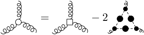
Figure 3: Truncated DSE for the three-gluon vertex, under the assumption of ghost dominance.

Possible tensor decompositions of the three-gluon vertex are given in Ref. (19). For sake of illustration, we confine ourselves to the form factor corresponding to the tensor structure of the bare three-gluon vertex

$$f_{3A}\mathrel{\mathop{:}}=\frac{\Gamma_{3}\cdot\Gamma_{3}^{(0)}}{\Gamma_{3}^{(0)}\cdot\Gamma_{3}^{(0)}},$$ (29)

where $\Gamma_{3}^{(0)}$ is the perturbative vertex, given by Eq. (28) with $\Omega({\bm{p}})$ replaced by $\lvert{\bm{p}}\rvert$. Furthermore, we consider a particular kinematic configuration, where two momenta have the same magnitude

$${\bm{p}}_{1}^{2}={\bm{p}}_{2}^{2}=p^{2},\quad{\bm{p}}_{1}\cdot{\bm{p}}_{2}=cp^{2}.$$ (30)

To evaluate the form factor $f_{3A}(p^{2},c)$, we use the ghost and gluon propagators obtained with a Gaussian wave functional (3) as input. The IR analysis of the equation for $f_{3A}(p^{2},c)$ [Eq. (29)] performed in Ref. (13) shows that this form factor should have a power law in the IR, with an exponent three times the one of the ghost dressing function; this is confirmed by our numerical solution (4). The result for the scalar form factor $f_{3A}$ for orthogonal momenta, $f(p^{2},0)$, is shown in Fig. 4, together with lattice results for $d=3$ Landau gauge Yang–Mills theory.

Figure 4: Form factor $f_{3A}$ of the three-gluon vertex for orthogonal momenta and comparison to lattice data for the $d=3$ Landau-gauge vertex (20). The momentum scale is arbitrary and has been adjusted to make the sign change occur at the same point. The lattice data are shown by courtesy of A. Maas.

Our result and the lattice data compare favorably in the low-momentum regime. In particular, in both studies, the sign change of the form factor occurs roughly at the same momentum where the gluon propagator has its maximum. (The scale in Fig. 4 is arbitrary.)

4 Hamiltonian flow

The advantage of the variational approach to the Hamiltonian formulation is its close connection to physics. The price to pay is the apparent loss of manifest renormalization group invariance. Renormalization group invariance is naturally built-in in the functional renormalization group approach to the Hamiltonian formulation of Yang–Mills theory proposed in ref. (5).

In the FRG approach the quantum theory of a field $\varphi$ is infrared regulated by adding the regulator term

$$\Delta S_{k}[\varphi]=\frac{1}{2}\varphi\cdot R_{k}\cdot\varphi\equiv\frac{1}{2}\int\varphi R_{k}\varphi$$ (31)

to the classical action, which in the Hamiltonian approach is given by the logarithm of the wave functional (24). The regulator function $R_{k}(p)$ is an effective momentum dependent mass with the properties

$$\lim\limits_{p/k\to 0}R_{k}(p)>0,\qquad\lim\limits_{k/p\to 0}R_{k}(p)=0,$$ (32)

which ensures that $R_{k}(p)$ suppresses propagation of modes with $p\lesssim k$ while those with $p\gtrsim k$ are unaffected and the full theory at hand is recovered as the cut-off scale $k$ is pushed to zero. Wetterich’s flow equation for the effective action $\Gamma_{k}[\phi]$ of a field $\phi$ is given by

$$k\partial_{k}\Gamma_{k}[\phi]=\frac{1}{2}\operatorname{Tr}\,\frac{1}{\Gamma_{k}^{(2)}[\phi]+R_{k}}\,k\partial_{k}R_{k},$$ (33)

$$\Gamma^{(n)}_{k,1\dots n}[\phi]=\frac{\delta^{n}\Gamma_{k}[\phi]}{\delta\phi_{1}\dots\delta\phi_{n}}$$ (34)

are the one-particle irreducible $n$-point functions (proper vertices). The generic structure of the flow equation (33) is independent of the details of the underlying theory, but is a mere consequence of the form of the regulator term (31), being quadratic in the field. By taking functional derivatives of Eq. (33) one obtains the flow equations for the (inverse) propagators and proper vertices. The general flow equation (33) still holds for the Hamiltonian formulation of Yang–Mills theory provided that $\phi$ is interpreted as the superfield $\phi=(\bm{A},c,\bar{c})$.

The FRG flow equations embody an infinite tower of coupled equations for the flow of the propagators and the proper vertices. These equations have to be truncated to get a closed system. We shall use the following truncation: we only keep the gluon and ghost propagators, which we write in the form

$$\Gamma^{(2)}_{k,AA}=2\omega_{k}(\bm{p}),\qquad\Gamma^{(2)}_{k,\bar{c}c}=\frac{p^{2}}{d_{k}(\bm{p})}\,.$$ (35)

In addition, we keep the ghost-gluon vertex $\Gamma^{(3)}_{k,A\bar{c}c}$, which we assume to be bare, i.e., we do not solve its FRG flow equation. Moreover, we shall assume infrared ghost dominance and discard gluon loops. Then the resulting flow equations of the ghost and gluon propagator reduce to the ones shown in Figs. 5 and 6.

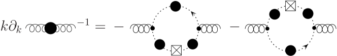
Figure 5: Truncated flow equation of the gluon propagator. The bare vertices at $k=\Lambda$ are symbolized by small dots and the regulator insertion $k\partial_{k}R$ by a crossed square.

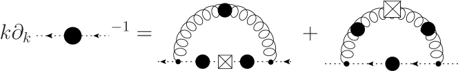
Figure 6: Truncated flow equation of the ghost propagator

These flow equations are solved numerically using the regulators

$$R_{A,k}(\bm{p})=2pr_{k}(\bm{p}),\qquad R_{c,k}(\bm{p})=p^{2}r_{k}(\bm{p}),$$ (36)

$$r_{k}(\bm{p})=\exp\left[\frac{k^{2}}{p^{2}}-\frac{p^{2}}{k^{2}}\right],$$ (37)

and the perturbative initial conditions at the large momentum scale $k=\Lambda$,

$$d_{\Lambda}(p)=d_{\Lambda}=\mathrm{const.}\,,\qquad\omega_{\Lambda}(p)=p+a.$$ (38)

With these initial conditions, the flow equations for the ghost and gluon propagators are solved under the constraint of infrared scaling for the ghost form factor. The resulting full flow of the ghost dressing function is shown in Fig. 7.

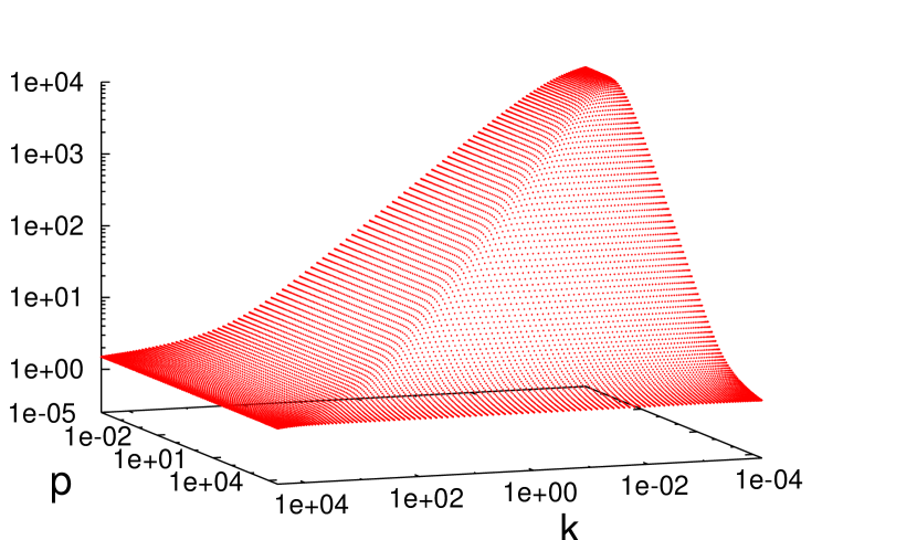
Figure 7: Flow $d_{k}(p)$ of the ghost form factor.

As the IR cut-off momentum $k$ is decreased, the ghost form factor $d_{k}(\bm{p})$ (constant at $k=\Lambda$) builds up infrared strength and the final solution at $k=k_{min}$ is shown in Fig. 9 together with the one for the gluon energy $\omega_{k_{min}}(\bm{p})$ in Fig. 8. It is seen that the IR exponents, i.e., the slopes of the curves $d_{k_{min}}(\bm{p})$, $\omega_{k_{min}}(\bm{p})$ do not change as the minimal cut-off $k_{min}$ is lowered. Let us stress that we have assumed infrared scaling of the ghost form factor but not the horizon condition $d_{k=0}^{-1}(p=0)=0$. The latter was obtained from the integration of the flow equation but not put in by hand (the same is also true for the infrared analysis of the Dyson–Schwinger equations following from the variational Hamiltonian approach, i.e., assuming scaling the DSEs yield the horizon condition).

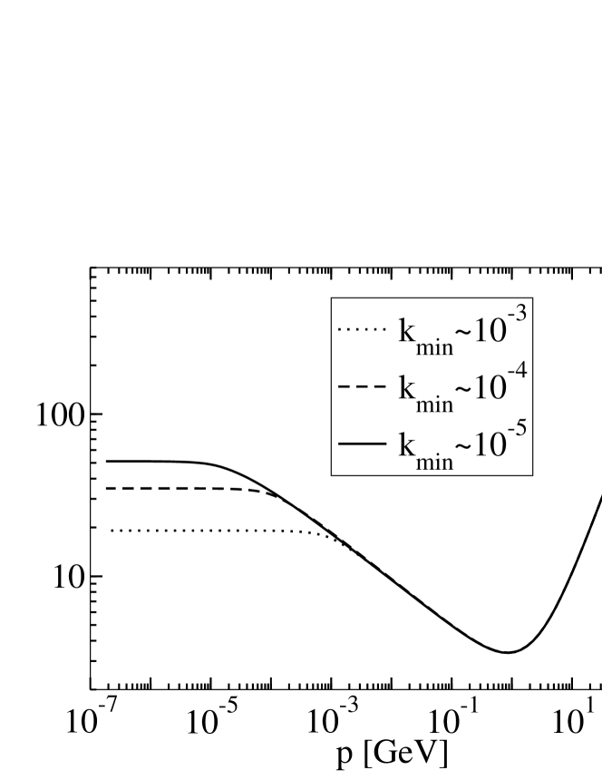
Figure 8: Inverse gluon propagator $\omega$ at three minimal cut-off values $k_{min}$.

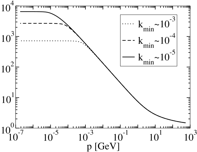
Figure 9: Inverse ghost form factor $d$ at three minimal cut-off values $k_{min}$.

The infrared exponents extracted from the numerical solutions of the flow equations are $\alpha=0{.}28$ and $\beta=0{.}64$. They satisfy the sum rule found in (13) resulting from the DSE obtained in the variational approach but are smaller than the ones of the DSE. Moreover, the present approach allows to prove the uniqueness of the sum rule (21) (5), analogously to the proof in Landau gauge (21).

Replacing the propagators with running cut-off momentum scale $k$ under the loop integrals of the flow equation by the propagators of the full theory,

$$d_{k}(\bm{p})\to d_{k=0}(\bm{p}),\qquad\omega_{k}(\bm{p})\to\omega_{k=0}(\bm{p}),$$ (39)

amounts to taking into account the tadpole diagrams (5). Then the flow equations can be analytically integrated and turn into the DSEs obtained in the variational approach (2), with explicit UV regularization by subtraction. This establishes the connection between these two approaches and highlights the inclusion of a consistent UV renormalization procedure in the present approach. The above results encourage further studies, which includes the flow of the potential between static color sources as well as dynamic quarks.

References

- Szczepaniak and Swanson (2001) A. P. Szczepaniak, and E. S. Swanson, Phys. Rev. D65, 025012 (2001), hep-ph/0107078.
- Feuchter and Reinhardt (2004) C. Feuchter, and H. Reinhardt, Phys. Rev. D70, 105021 (2004), hep-th/0408236.
- Epple et al. (2007) D. Epple, H. Reinhardt, and W. Schleifenbaum, Phys. Rev. D75, 045011 (2007), hep-th/0612241.
- Campagnari and Reinhardt (2010) D. R. Campagnari, and H. Reinhardt, Phys. Rev. D82, 105021 (2010), 1009.4599.
- Leder et al. (2011) M. Leder, J. M. Pawlowski, H. Reinhardt, and A. Weber, Phys. Rev. D83, 025010 (2011), 1006.5710.
- Christ and Lee (1980) N. H. Christ, and T. D. Lee, Phys. Rev. D22, 939–958 (1980).
- Campagnari et al. (2009) D. R. Campagnari, H. Reinhardt, and A. Weber, Phys. Rev. D80, 025005 (2009), 0904.3490.
- Reinhardt and Feuchter (2005) H. Reinhardt, and C. Feuchter, Phys. Rev. D71, 105002 (2005), hep-th/0408237.
- Reinhardt (2008) H. Reinhardt, Phys. Rev. Lett. 101, 061602 (2008), 0803.0504.
- Reinhardt and Epple (2007) H. Reinhardt, and D. Epple, Phys. Rev. D76, 065015 (2007), 0706.0175[hep-th].
- Reinhardt and Schleifenbaum (2009) H. Reinhardt, and W. Schleifenbaum, Annals Phys. 324, 735–786 (2009), 0809.1764.
- Burgio et al. (2009) G. Burgio, M. Quandt, and H. Reinhardt, Phys. Rev. Lett. 102, 032002 (2009), 0807.3291.
- Schleifenbaum et al. (2006) W. Schleifenbaum, M. Leder, and H. Reinhardt, Phys. Rev. D73, 125019 (2006), hep-th/0605115.
- Feuchter and Reinhardt (2008) C. Feuchter, and H. Reinhardt, Phys. Rev. D77, 085023 (2008), 0711.2452.
- Burgio et al. (2010) G. Burgio, M. Quandt, and H. Reinhardt, Phys. Rev. D81, 074502 (2010), 0911.5101.
- Yamamoto and Suganuma (2010) A. Yamamoto, and H. Suganuma, Phys. Rev. D81, 014506 (2010), 0911.5391.
- Campagnari et al. (2011) D. Campagnari, A. Weber, H. Reinhardt, F. Astorga, and W. Schleifenbaum, Nucl. Phys. B842, 501–528 (2011), 0910.4548.
- Fischer et al. (2009) C. S. Fischer, A. Maas, and J. M. Pawlowski, Annals Phys. 324, 2408–2437 (2009), 0810.1987.
- Ball and Chiu (1980) J. S. Ball, and T.-W. Chiu, Phys. Rev. D22, 2550 (1980).
- Cucchieri et al. (2008) A. Cucchieri, A. Maas, and T. Mendes, Phys. Rev. D77, 094510 (2008), 0803.1798.
- Fischer and Pawlowski (2009) C. S. Fischer, and J. M. Pawlowski, Phys. Rev. D80, 025023 (2009), 0903.2193.