Mapping differential reddening in the inner Galactic globular cluster system

Abstract

A serious limitation in the study of many globular clusters – especially those located near the Galactic Center – has been the existence of large and differential extinction by foreground dust. In a series of papers we intend to map the differential extinction and remove its effects, using a new dereddening technique, in a sample of clusters in the direction of the inner Galaxy, observed using the Magellan 6.5m telescope and the Hubble Space Telescope. These observations and their analysis will let us produce high quality color-magnitude diagrams of these poorly studied clusters that will allow us to determine these clusters’ relative ages, distances and chemistry and to address important questions about the formation and the evolution of the inner Galaxy. We also intend to use the maps of the differential extinction to sample and characterize the interstellar medium along the numerous low latitude lines of sight where the clusters in our sample lie. In this first paper we describe in detail our dereddening method along with the powerful statistics tools that allow us to apply it, and we show the kind of results that we can expect, applying the method to M62, one of the clusters in our sample. The width of the main sequence and lower red giant branch narrows by a factor of 2 after applying our dereddening technique, which will significantly help to constrain the age, distance, and metallicity of the cluster.

1 Introduction

The age, chemical and kinematic distributions of Galactic stellar populations provide powerful constraints on models of the formation and evolution of the Milky Way. The Galactic globular clusters (GGC) constitute an especially useful case because the stars within individual clusters are coeval and spatially distinct. But uncertainties in the determination of distances to GGCs, along with uncertainties in the determination of their physical characteristics such as age or metallicity can result when the reddenig produced by interstellar dust is not properly taken into account (Calamida et al., 2005). In this context, differential reddening across the field of the cluster has proven to be difficult to map, and the properties of GGCs that suffer high and patchy extinction, especially those in the direction of the inner Galaxy, have not been accurately measured (Valenti et al., 2007).

Several authors have used different methods to try to map differential extinction in GGCs before: Piersimoni et al. (2002) have used colors of variable RRLyrae stars to create the reddening maps; Melbourne & Guhathakurta (2004) and Heitsch & Richtler (1999) have used photometric studies of the stars in the horizontal branch (HB); von Braun & Mateo (2001) and Piotto et al. (1999b) have used photometric studies of main sequence (MS), subgiant branch (SGB), and red giant branch (RGB) stars.

In this paper we describe a new dereddening technique, based on this last approach, but with the improvement of calculating the extinction not on a predetermined grid but on a star by star basis. In section 2 we extensively explain this dereddening method and in section 3 we apply it to an example cluster, M62. In the next papers of this series we plan to apply this dereddening method to a sample of clusters in the direction of the inner Galaxy that in principle can be affected by this effect, and analyze the obtained results. In Paper II we will present a new photometric database consisting of a sample of 25 inner GGCs observed using the Magellan 6.5m telescope and the Hubble Space Telescope (HST), describe the processes we follow to obtain an accurate astrometric and photometric calibration of the stars in these clusters, and, after applying the dereddening technique, give the extinction maps along the field of the clusters in the sample, along with new cleaner, differentially dereddened color-magnitude diagrams (CMD) of these GGCs. In Paper III we will provide an analysis of the stellar populations of these clusters based on their dereddened CMDs. Finally, in Paper IV, we will characterize the interstellar medium along the low-latitude lines of sight were the clusters lie, based on the properties of the extinction maps we derived.

2 Dereddening technique

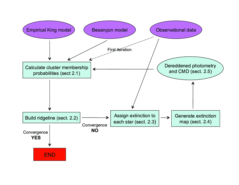
Figure 1: Flow chart describing our technique to map the differential extinction.

Our dereddening technique is composed of five iterative steps (see figure 1):

• We assign a probability to the stars in our observed regions to belong to the cluster or to the Galactic field depending on their positions in the sky and in the CMD (see section 2.1).

• We build a ridgeline for the stellar population of the observed cluster. The ridgeline represents the evolutionary path that a given star is going to follow in the CMD (see section 2.2).

• We assign an individual extinction value to every star, based on its displacement from the ridgeline along the reddening vector (see section 2.3).

• We smooth the different individual color excesses over the observed field to generate an extinction map (see section 2.4).

• We apply the extinction values from the map to the stars in our observations to construct a dereddened CMD (see section 2.5).

We repeat these steps iteratively. Every iteration the ridgeline is more accurately defined, and therefore the extinction map and the dereddened CMD are also more precise. We end up the process when there is a convergence in the calculated ridgeline.

This technique is based on work by von Braun & Mateo (2001) and Piotto et al. (1999b), and pioneered by Kaluzny & Krzeminski (1993), but unlike them, we do not divide the field in a grid of well established subregions a priori, but use a non-parametric approximation to smooth the information about the reddening in the field provided by every star, without such hard edges.

The success of this analysis depends critically on the assumption that the stellar populations are uniform within individual GCs. Recent studies tend to suggest that this is not strictly true, especially in the most massive GGCs and GGCs with an extreme blue horizontal branch (EBHB) (Bedin et al., 2004; Piotto et al., 2007). In the cases discovered, it is conjectured that the spread in helium content between stars in the cluster is important, but the spread in age and metallicity seems to be small (D’Antona & Caloi, 2008), making the spread of the stars in the SGB and upper RGB regions of the CMD also small. Since most of the information in our method comes from stars in these regions of the CMDs, our technique should not be significantly affected. What is more, in our method variations in the reddening must be spatially related, which should not be the case if there are multiple helium enriched populations within the cluster. Because of these reasons and since our sample only includes a few massive and EBHB clusters, we expect the differential populations effects to be comparatively minor and not significantly affect our dereddening approach.

Also it is important to realize that our dereddening method does not establish the absolute extinction toward a target cluster, so to estimate the absolute extinction in each case we need to use other methods, e.g., comparison of our differentially dereddened CMDs with isochrone models, or use of reddening estimates from RR Lyr stars in our fields.

2.1 Field-cluster probability assignment

From our photometric studies we can assign probabilities to the stars in our observations to belong to the clusters, based on $r$, their position in the sky with respect to the center of the cluster, and also on ($c,m$), their color and magnitude position on the CMD. These probabilities will be used in the next steps of our technique to give higher weight to the information provided by stars with high probabilities of being cluster members.

Before going any further, it is convenient to explain the notation that we are going to use, and to remember the basic rules of probability calculation. The marginal or unconditional probability of an event A happening is expressed $P(A)$. The joint probability of an event A and an event B happening at the same time is expressed $P(A,B)$. Finally, the conditional probability of an event A happening given the occurrence of some other event B is expressed $P(A|B)$, and can be written as

$$P(A|B)=\frac{P(A,B)}{P(B)}$$ (1)

or, using Bayes theorem, as

$$P(A|B)=\frac{P(B|A)P(A)}{P(B)}$$ (2)

Also, notice that in many parts of our analysis it is going to be more convenient to use probability density functions, $\rho(x)$, to express the probability. These functions describe the relative likelihood for a random variable X to occur at a given point in the sampled space $\Omega$ and satisfy

$$P(a\leq X\leq b)=\int^{b}_{a}\rho(x)dx$$ (3)

$$For\ all\ x:\rho(x)\geq 0$$ (4)

$$\int_{\Omega}\rho(x)dx=1$$ (5)

Whenever needed in this work, the probability density functions are calculated non-parametrically using locfit. Locfit (Loader, 1999) is a local likelihood estimation software implemented in the R statistical programming language (see appendix). Locfit does not constrain the probability density functions globally, i.e., it is non-parametric, but assumes that locally, in a local window around a certain point in the sample space, the functions can be well approximated by a polynomial. Hence the main inputs that locfit requires are the positions of the observed elements in the sample space, and a parameter to define the local window where the function is approximated parametrically, i.e., a smoothing factor given by the maximum of two elements: a bandwidth generated by a nearest neighbor fraction, and a constant bandwidth.

Now, if we suppose the variable $X$ indicates membership to the cluster ($X=1$ indicates observation of a member, and $X=0$ indicates observation of a non-member), in the next paragraphs we calculate $P(X=1|r,c,m)$, the conditional probability of the stars being members of the cluster, given their position in the sky and in the CMD. Actually, it is more convenient for us to calculate first $P(X=1|r)$ and $P(X=1|c,m)$, the conditional probabilities of the stars to belong to the cluster given just their position in the sky, and just their position in the CMD, and only after attempt to calculate $P(X=1|r,c,m)$.

The conditional probability of the stars being members of the cluster, given just their position in the sky as a function of the distance to the center of the cluster, $P(X=1|r)$, can be written, using Bayes theorem, as

$$P(X=1|r)=\frac{{\rho}(r|X=1)P(X=1)}{{\rho}(r)}$$ (6)

For any given cluster, both ${\rho}(r|X=1)$ and $P(X=1)$ are unknown. But since $P(X=1)$ is the ratio of the observed cluster stars to the total observed stars, we can rewrite $eq.\ 6$ as

$$P(X=1|r)=\frac{s_{mem}(r)}{s_{t}(r)}$$ (7)

where $s_{mem}(r)$ is the number of observed member stars as a function of the distance to the cluster center, and $s_{t}(r)$ is the total number of observed stars as a function of the distance to the cluster center. We still do not know $s_{mem}(r)$, but if we divide both numerator and denominator in $eq.\ 7$ by $A(r)$, the area coverage at a given $r$ of the field of view (FOV) in our observation of the cluster, we can rewrite $eq.\ 7$ as

$$P(X=1|r)=\frac{f_{mem}(r)}{f_{t}(r)}$$ (8)

where $f_{mem}(r)$ is the surface density of observed member stars as a function of the distance to the cluster center, and $f_{t}(r)$ is the total surface density of observed stars as a function of the distance to the cluster center. Now, if we assume an empirical King profile (King, 1962) for the cluster, we can write the surface density of member stars as

$$f_{mem}(r)=kK(r)=k\left\{\begin{array}[]{rcl}\left(\frac{1}{[1+(r/r_{c})^{2}]^{1/2}}-\frac{1}{[1+(r_{t}/r_{c})^{2}]^{1/2}}\right)^{2}&\mbox{if}&r\leq r_{t}\\ 0&\mbox{if}&r>r_{t}\end{array}\right.$$ (9)

where $r_{c}$ and $r_{t}$ are the core radius and the tidal radius of the cluster. If we make another assumption and consider a constant surface density of stars for the non-member population, which is reasonable due to the small size of our field, then

$$f_{non}(r)=c$$ (10)

and we have the following functional form for the total surface density distribution of stars observed in our FOV

$$f_{t}(r)=kK(r)+c$$ (11)

and, according to $eq.\ 8$, we can write the conditional probability of the stars being members of the cluster, given their position in the sky, as

$$P(X=1|r)=\frac{kK(r)}{kK(r)+c}$$ (12)

or, alternatively,

$$P(X=1|r)=1-P(X=0|r)=1-\frac{c}{kK(r)+c}$$ (13)

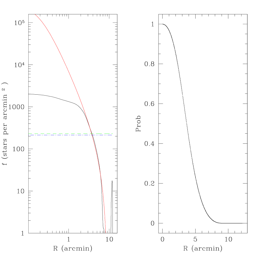
Figure 2: On the left, the density distribution per area of the stars in M 62 as a function of distance to the GC center, minus the constant density distribution found for the field (dashed green line), is plotted as the solid black line, while the King model for the cluster is plotted with a red solid line, and the constant density distribution of stars in the field provided by the Besançon model is shown as a blue dashed line (see table 1 for the parameters used to build and fit the model). On the right, $P(X=1|r)$, the probability of the stars to belong to the cluster as a function of distance from the cluster center.

Therefore to calculate $P(X=1|r)$ we need to find the coefficients $k$ and $c$, since $K(r)$ can be obtained taking the values for $r_{c}$ and $r_{t}$ for every cluster in our sample provided in the Harris catalog (Harris, 1996). These two remaining coefficients, $k$ and $c$, can be easily found by a least squares fit of $K(r)$ to the observed surface density of stars $f_{t}(r)$ (see $eq.\ 11$, figure 2, and table 1). To find the observed $f_{t}(r)$, we need to first calculate the number of stars $s_{t}(r)$, and then divide it by the area coverage $A(r)$. As we mentioned when passing from $eq.\ 6$ to $eq.\ 7$, the number of stars $s_{t}(r)$ is just the probability density ${\rho}(r)$ of stars in our observation, multiplied by the total number of observed stars. We calculated the probability density ${\rho}(r)$ of stars by feeding locfit with the radial positions of the stars and a smoothing factor with a constant bandwidth of 0.25 arcmin. The surface coverage $A(r)$ in our observation is not trivial to find, since our FOV is a square not centered in the cluster center. In order to quickly calculate this area, we create a grid of points equally spaced over our FOV, calculate the probability density ${\rho}(r)$ of points, and then multiply by the area of the FOV. We calculated the probability density ${\rho}(r)$ of points by feeding locfit with the radial positions of the points in the grid and a smoothing factor with a constant bandwidth of 0.25 arcmin.

The conditional probability of the stars being members of the cluster, given just their position in the color magnitude diagram, $P(X=1|c,m)$, can be written, using Bayes theorem, as

$$P(X=1|c,m)=\frac{{\rho}(c,m|X=1)P(X=1)}{{\rho}(c,m)}$$ (14)

For any given cluster, we do not know the true distribution in magnitude and color in our observations of genuine GC members, but we can model the distribution of the field, non-member stars. We use the model of the Galaxy described in Robin et al. (2003), from now on referred as the ’Besançon model’, to obtain ${\rho}(c,m|X=0)$. We can now rewrite $eq.\ 14$ as

$$P(X=1|c,m)=1-P(X=0|c,m)=1-\frac{{\rho}(c,m|X=0)P(X=0)}{{\rho}(c,m)}$$ (15)

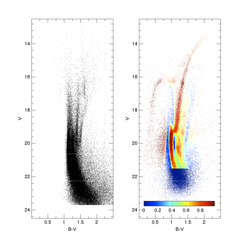
Figure 3: On the left, CMD from the Besançon model of the Galactic stars in the field centered in the cluster position (see table 2 for the parameters used to build the model). On the right, our observed CMD, with the cluster belonging probabilities as a function of color and magnitude, $P(X=1|c,m)$, represented by the different colors of the stars as indicated in the colorbar. Notice that we restrict our analysis to stars brighter than the completeness limit shown in table 3.

where ${\rho}(c,m|X=0)$ is obtained feeding locfit with the position in the CMD of the Galactic field stars provided by the Besançon model and a smoothing factor with a nearest neighbor ratio of 0.01, ${\rho}(c,m)$ is obtained feeding locfit with the position in the CMD of the stars in our observations and a smoothing factor with a nearest neighbor ratio of 0.01, and $P(X=0)$ is just the ratio of the total number of modeled non-member stars for an area equal to the FOV of the observation, to the total number of observed stars, which include field and cluster stars. To take care of the different variation ranges in color and in magnitude for the stars in the CMD a scale (see appendix) of 1 in color to 5 in magnitude is also provided to locfit as an input parameter to calculate ${\rho}(c,m|X=0)$ and ${\rho}(c,m)$. In figure 3 we can see the different $P(X=1|c,m)$ for the stars in M62, one of the clusters in our sample. Similar methods to calculate $P(X=1|c,m)$ have been employed by Hughes et al. (2007) based on calculations by Hughes & Wallerstein (2000) and Mighell et al. (1998), and also by Law et al. (2003) based on calculations by Odenkirchen et al. (2001) and Grillmair et al. (1995). In contrast to these other studies we do not eliminate stars from our analysis based on these probabilities, but downweight them. Also, as we show at the end of this section, we do not just use $P(X=1|c,m)$, but $P(X=1|r,c,m)$ in our following analysis.

Given the importance of the Besançon model (and the CMDs it provides) in analyzing the Galactic field component of our observations and calculating $\rho(c,m|X=0)$, we describe here in more detail the input parameters that we use in the web interface of the Besançon group to model the non-member stellar populations in the vicinity of the sampled clusters.

• Field of view. We use the small field option from the web interface, in which the modeled stars are all supposed to be at the same coordinates (see table 2), implicitly assuming that the field star density gradient across the FOV is negligible. The same assumption was made in the calculation of $f_{non}(r)$ (see $eq.\ 10$). To obtain higher statistical significance in the models, we can increase the selection area to obtain a larger number of stars in the model. ${\rho}(c,m|X=0)$ is independent of the area and the number of stars used, since it is normalized (see $eq.\ 5$). In practice, we set this parameter to select $\sim 300000$ stars (see table 2). We have to notice though, that when calculating $P(X=0)$ in $eq.\ 15$ we need to normalize the number of stars in the model to the FOV.

• Extinction law. We apply locfit to map ${\rho}(c,m)$ as a function of $c$ and $m$ using the CMDs from our observations. From the modeled stars, we can also use locfit to map ${\rho}(c,m|X=0)$ as a function of $c$ and $m$, realizing that this map changes depending on what extinction $A_{V}$ we assumed for our modeled data. So if we define $g_{ext}$ as

  $$g_{ext}=\sum_{c,m}[{\rho}(c,m){\rho}(c,m|X=0)]$$ (16)

  we need to realize that this function depends also on the extinction assumed for the modeled CMDs, i.e., $g_{ext}(A_{V})$. For the fields studied, we choose the modeled stars to simulate no interstellar extinction in the beginning. Then we move the density maps of the models along the reddening vector in increments of extinction ${\Delta}A_{V}=0.01$, calculating $g_{ext}$ for every increment. The value of $A_{V}$ where $g_{ext}$ is a maximum is the value we choose for the absolute extinction of our observation. This $A_{V}$ is generally equal or within a few hundredths of a magnitude to the one provided in Harris (1996). The extinction is then simulated in the model as a cloud with an extinction equal to this $A_{V}$ at distance of 0 pc (see table 2).

• Characteristics of the stars used in the model. We allow all ages, Galactic components, and spectral types provided by the Besançon model. We provide a limit only in the intervals of magnitudes, equal to the ones of our observations (table 2). We also model our observational errors ${\sigma}_{ph}$ with an exponential function of the apparent magnitude m in each band:

  $${\sigma}_{ph}=A+exp(Cm-B)$$ (17)

  so the models will take the photometric error into account providing a more realistic approximation (see table 2).

Certain problems arise in this procedure of calculating the conditional probabilities $P(X=1|r)$ and $P(X=1|c,m)$, including:

• We have to take into account the completeness factor of our photometric observations. In general, completeness decreases with magnitude somewhat smoothly at the faint end, but suddenly at the saturation limit. Because of this, and since we are trying to calculate the probabilities comparing our observations with models (King profile and Besançon model) we need to find where the completeness factor starts to decrease at the faint end. Usually this is done with artificial-star tests, injecting stars in the CMD and analyzing the amount and magnitudes of the ones recovered (Piotto et al., 1999a). But our large sample and large cluster star density gradients within individual fields make artificial star tests highly inefficient, so we explore another method that is well-suited to our specific fields, and also much more efficient to implement. From the Besançon model we can calculate the number of non-member stars per area in the field that we have in a given magnitude range, and from our data we can also find the number of non-member stars per area in the field in a given magnitude range just by fitting $eq.\ 11$ in that magnitude range. So we iteratively calculate both numbers making the magnitude range smaller taking away stars in the 0.1 mag fainter end every time we do the calculation, repeating the process until we are able to get the cumulative luminosity functions (LF) for the seven fainter magnitudes for the non-member stars from every one of our pointings. Then we can compare the modeled and observed LFs to see where the functions deviate one from the other. But this approximation proves to be not very accurate, especially in cases in which the number of non-member stars in the field is small. Instead we explore yet another approximation. We notice that the LF in the Besançon model is always a concave function, while the observed LF of the non-member stars in the field becomes a convex function at the faint end. We can then identify the limit where the completeness factor starts to decrease as the inflection point where the observational cumulative LF changes from concave to convex. The inflection point is the point where the derivative of the LF has a extreme, a minimum in our cases. And the derivative is easily found using locfit to calculate non-parametrically the LF and its derivative (see appendix). The completeness limit is usually located in our observations at $\sim 2$ magnitudes from the faint end in $V$ (see table 3). In the next steps of our dereddening method we only use stars brighter than this limit.

• The completeness factor also depends on the distance to the center of the cluster, strongly so for the more crowded cases. Close to the cluster center we are not only missing stars at the faint end of the magnitude distribution, but at all magnitudes, since the lower completeness factor in this region is mostly caused by masking saturated regions by DoPHOT (Schechter et al., 1993), the program used to do the photometric analysis of the images. From the calculation of the $P(X=1|r)$, we can see that this reduced completeness factor reveals itself as a deviation from the model fit shown in $eq.11$ at distances close to the center of the cluster (see figure 2). If we assume that we are missing an equal percentage of stars from the cluster and from the field, we can calculate its effect as the ratio between the observed and modeled $f_{t}(r)$. In the CMD, this lower completeness factor can lead to a miscalculation of $P(X=1|c,m)$ if the FOV is small. However, since the area of the regions whose extinction we are able to map are much bigger than the areas where the reduced completeness factor is an issue, the comparison of our observations with the Besançon model is not significantly affected. The only appreciable consequence is that the calculated $P(X=0)$ is a little higher than the actual $P(X=0)$. But this high value for $P(X=0)$ can be corrected if when we calculate the number of stars, we take into account the deviation of the observation from the model fit as a function of the distance to the center of the cluster, as we mentioned before.

• $P(X=1|r)$ is obtained using the values for the core and tidal radii provided in the Harris catalog (Harris, 1996), for every cluster in our sample. Notice that these values are not all of equal accuracy. Small variations in the initially adopted $r_{c}$ and $r_{t}$ could produce small changes in the individual $P(X=1|r)$ values, but they will not alter the general trend (stars closer to the center of the cluster have higher $P(x=1|r)$ than stars located further away), and therefore they will not significantly affect the result of our dereddening technique.

• $P(X=1|c,m)$ is obtained comparing a real observation with a model, where photometric errors are incorporated by mimicking the real photometric errors by the exponential function described above. In general, we observe that stars from the models tend to be a little more concentrated along the different field evolutionary sequences in the CMDs than stars from real observations. Therefore, for a given magnitude, $\rho(c,m|X=0)$ peaks higher and decreases faster in the model than in the real observation, producing two main errors in our calculations of $P(X=1|c,m)$. The first error is that we mistakenly assign a probability of being in the field which is too low, and therefore a probability of being cluster members which is too high, to stars in the regions where the observed color is an extreme for a given magnitude (see figure 3). But since there are not many stars in these regions and they usually have higher photometric errors in color than our functions describe, they are downweighted or removed from our calculations later on (see section 2.4). More important is the second error, the case were $\rho(c,m|X=0)$ peaks higher in the model than in reality, making the probability of the star to be a non-member in the field too high, and $P(X=1|c,m)$ too low, lower than 0. In order to avoid these non-physical cases, and even too extreme cases that can give too low a weight value to the information coming from those stars, we put the hard limit $P(X=1|c,m)\geq 0.1$ (see figure 3).

Now we are in conditions to calculate $P(X=1|r,c,m)$, the conditional probability of the stars being members of the cluster given both their position in the sky and in the CMD. According to Bayes theorem,

$$P(X=1|r,c,m)=1-P(X=0|r,c,m)=1-\frac{{\rho}(r,c,m|X=0)P(X=0)}{{\rho}(r,c,m)}$$ (18)

and since the positions in the sky and in the CMD for non-member stars are independent

$$P(X=1|r,c,m)=1-\frac{{\rho}(r|X=0){\rho}(c,m|X=0)P(X=0)}{{\rho}(r,c,m)}$$ (19)

and using Bayes theorem again (see $eq.\ 6$) we can write

$$P(X=1|r,c,m)=1-\frac{{\rho}(c,m|X=0){\rho}(r)P(X=0|r)}{{\rho}(r,c,m)}$$ (20)

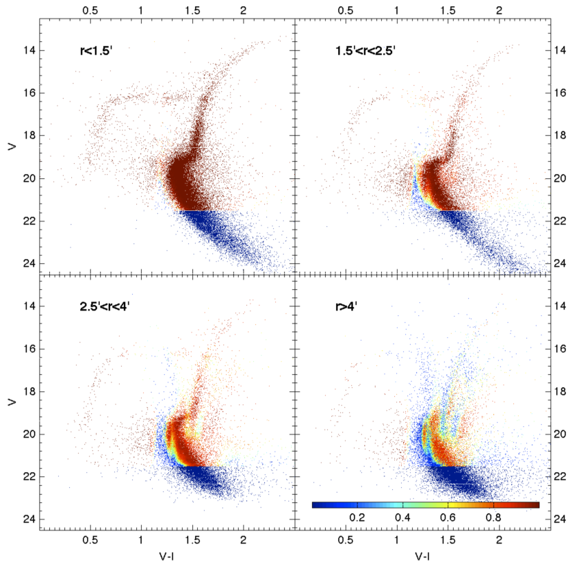
Figure 4: Our observed dereddened CMD at four different distances from the cluster center, with the probability of every star to belong to the cluster as a function of position in the sky, color and magnitude, $P(X=1|r,c,m)$, represented by the different colors of the stars as indicated in the colorbar. Notice that we restrict our analysis to stars brighter than the completeness limit shown in table 3.

$P(X=0|r)$, ${\rho}(r)$, and ${\rho}(c,m|X=0)$, the three elements in the numerator have been calculated previously, so now we just need to find the denominator ${\rho}(r,c,m)$, the probability density of stars in our observation as a function of both position in the sky and in the CMD. To calculate it we feed locfit with the position in the sky and in the CMD of the stars in our observations and a smoothing factor with a nearest neighbor ratio of 0.1. Since the units of the three physical magnitudes $r,c,m$ are different, we need to feed locfit with a scale factor (see appendix) to calculate the distance between neighbors in the $r,c,m$ space. Experimentally we found that a scale of 1 magnitude in color to 5 magnitudes in brightness and 10 arcmin in distance to the the GC center provides good results, and it is the one we used as an input parameter of locfit to calculate ${\rho}(r,c,m)$. The results of the $P(X=1|r,c,m)$ calculation are shown in figure 4. We can observe that the same problems that were previously mentioned affecting the calculation of $P(X=1|r)$ and $P(X=1|c,m)$ are present here. But for most of the stars observed, this formalism allows a more precise way to discriminate between field and cluster stars than looking to just $P(X=1|r)$ or just $P(X=1|c,m)$.

2.2 Building the ridgeline

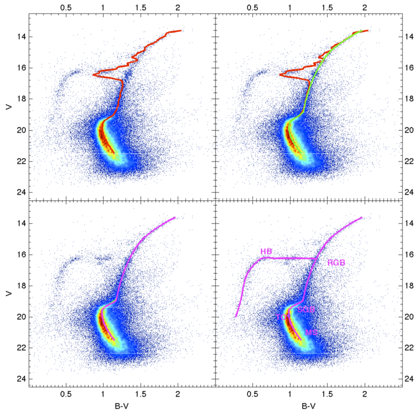
Figure 5: CMD of the example GC, M 62, with the ridgeline provided after the first (upper left), second (upper right), and third (lower left) iterations of our method. Warmer (redder) colors mean higher density of stars in a region of the CMD. On the lower right, the HB ridgeline is also shown, along the different parts of the CMD morphology: main sequence (MS), turn-off point (TO), subgiant branch (SGB), red giant branch (RGB) and horizontal branch (HB).

Stars that are still alive in globular clusters evolve along the CMD following a well determined path. They spend most of their lives in the MS burning hydrogen in their core. They leave the MS at the turn-off point (TO) growing in size and burning hydrogen in a shell as they move across the SGB and the RGB. Then they move to the HB where they burn helium in the core and hydrogen in a shell. They leave the HB moving across the asymptotic giant branch (AGB) burning helium and hydrogen in a shell, then moving rapidly across the post AGB phases to finish their lives as white dwarfs (WD). The path of this standard evolutionary sequence in the CMD of a globular cluster is shown in figure 5.

We try to model the first stages (MS, SGB and RGB) of the evolutionary path followed by the stars in a GC building the ridgeline for the CMDs of the GGCs, using locfit to construct a univariate non-parametric regression of the color of the stars as a function of the magnitude. This process is composed of three iterations.

In the first iteration, we carry out a non-parametric regression in the whole CMD to obtain a first estimation of the cluster ridgeline as a function of magnitude. We feed locfit with the magnitudes and colors of the stars and a smoothing parameter with a constant bandwidth of 0.2 magnitudes. Also, we give locfit preliminary weights for the stars

$$W=P(X=1|r,c,m)w_{ph}$$ (21)

where $P(X=1|r,c,m)$ is the membership probability calculated in the previous subsection and $w_{ph}$ is a photometric weight equal to the inverse of the square of the Poisson error of the photometric magnitude $w_{ph}=1/{\sigma}^{2}_{V}$. These preliminary weights $W$ are calculated to favor the magnitude and color information provided by stars with more accurate photometry and higher probability of being cluster members according to both their position in the sky and in the CMD. The smoothing parameter values used have proven experimentally to be adequate for describing the MS and part of the RGB, but the regression fails to describe the SGB, and the stars in the HB create problems when trying to model the whole RGB. Still, they produce a reasonable first approximation (see upper left plot in figure 5) and let us identify the TO point, which we define as the bluest point of our ridgeline. We should note here that the MS is defined not to the faintest magnitude limit of the data, but to the completeness limit defined in section 2.1.

In the second iteration we try to get a less noisy whole ridgeline, along with a better defined RGB ridgeline. As a first step we divide the initial ridgeline in three regions: the MS region, where the ridgeline magnitudes are $m>m_{TO}$, the SGB region, where the ridgeline magnitudes are $m_{TO}-1\leq m\leq m_{TO}$, and the RGB region, where the ridgeline magnitudes are $m<m_{TO}-1$. To smooth out the approximation for the ridgeline, we take the points from the ridgeline from the first iteration for every region and smooth them using locfit with a nearest neighbor ratio of 0.7 (locfit default), no preliminary weights or constant bandwidth requirements. The RGB ridgeline is still not well defined, because of the effects of stars in the HB. To calculate a better ridgeline for the RGB getting rid of the effects of the blue part of the HB, we take only stars in the magnitude range $m<m_{TO}-1$ and in the color range $col_{TO}<col$. We feed locfit with their magnitudes and colors, and a constant bandwidth of 0.2 mag and a nearest neighbor ratio of 0.1 to calculate the smoothing parameter. We use the nearest neighbor ratio because if not, the upper part of the RGB, usually scarcely populated, can become very noisy. Still, the red part of the HB, whenever present, is going to deviate the calculated RGB ridgeline. To eliminate its effect we have to locate first where the HB is. We look for a change in the sign of the slope of the RGB. The bluest point brighter than the point where the slope sign change is, shows where the HB is. And the difference between these two points provides information about the thickness of the HB, $m_{HBthickness}$. Once the HB is located, we repeat the analysis done before for the RGB, with the same smoothing parameter and weights, but now omitting points in the interval $m_{HB}-m_{HBthickness}\leq m\leq m_{HB}+m_{HBthickness}$. That way we have a better ridgeline for the upper and lower regions of the RGB. To get a ridgeline for the whole RGB, smoothing any noisy part, we follow a similar process to what we do in the beginning of this second iteration. We take the points in the description of the upper and lower RGB ridgeline, and use locfit again, but now with a nearest neighbor ratio of 0.7, no preliminary weights or constant bandwidth requirements. The ridgeline is much better now, but still we are a little off in the description of the SGB (see upper right plot in figure 5).

In the final iteration, we try to calculate a better ridgeline for the SGB. In order to do that we follow Marín-Franch et al. (2009), where they use rotated histograms to recalculate the ridgeline for the GC in their sample, using only stars perpendicular to the ridgeline in the calculation. Although our approximation is similar, the implementation is a little different. We calculate the slope of the curve at every point of the previously calculated ridgeline using locfit to get the derivative of the slope at a given point of the ridgeline. Once we have this, we rotate the coordinate system of every star at every magnitude with the angle $\alpha_{i}$ of the slope of the ridgeline at that magnitude, and centered at the ridgeline. Once this is done, we can get a ridgeline in the new coordinate system using locfit again. This new ridgeline should be a straight line along the Y coordinate with a value of 0 in the X coordinate. Any deviation from that means that the ridgeline in the original color-magnitude coordinate system requires a more accurate calculation. Notice that in order for the new coordinate system to consistently show these deviations, we need the range of both coordinates to be similar in the old coordinate system. This is not the case for the range of colors and magnitudes presented in a CMD. To try to get them to a similar scale we multiply the color by a factor of 5 before doing the rotation. In the calculation of the ridgeline in the new coordinate system the preliminary weights and smoothing factor used for locfit are the same as in the first iteration. We observe that the X coordinate of the ridgeline in the new reference system does not deviate significantly from 0 in the region of the MS stars, but does so in the SGB and upper RGB region. In the RGB region it is expected due to the scarcity of the population there. We took care of that in the previous iteration, so we concentrate our attention in the SGB region. We derotate the ridgeline in that region (the part where the original magnitudes are in the range $m_{TO}-1<m<m_{TO}$) to get their coordinates in the color-magnitude coordinate system, and after smoothing out any noise using locfit with a nearest neighbor ratio of 0.7, we put together the different parts of the ridgeline (see lower left plot in figure 5). The new ridgeline seems to follow accurately the different evolutionary sequences present in the GCs, and serves as the basis of our subsequent analysis.

In section 2.4 we discuss how we can use stars in the HB to test the accuracy of our method. To carry this test, we need to model a ridgeline for this region too. The process to find the ridgeline here is a little more interactive than for the other regions of the CMD. First, we have to decide by visual inspection of the CMD if we are dealing with a cluster that has only blue, only red or both sections of the HB. If the cluster shows only a blue HB, we carry out a non-parametric regression on the stars bluer than the TO to obtain an estimation of the cluster HB ridgeline as a function of magnitude. We feed locfit with the magnitudes and colors of the HB, and a constant bandwidth of 0.2 mag and a nearest neighbor ratio of 0.1 to calculate the smoothing parameter. If only a red HB is present instead, the non-parametric regression is performed on stars in the interval $m_{HB}-m_{HBthickness}\leq m\leq m_{HB}+m_{HBthickness}$ to obtain an estimation of the cluster HB ridgeline as a function of color. The smoothing parameter is calculated by locfit with the same parameters as for the blue HB. Finally, if the HB shows red and blue sections, we calculate both independently following the methods previously described, and then we smooth the result as a function of color, feeding locfit with the magnitudes and colors of the points in the description of the blue and red HB ridgeline, and a nearest neighbor ratio of 0.25, no preliminary weights or constant bandwidth requirements (see lower right plot in figure 5).

2.3 Calculating an extinction for every star

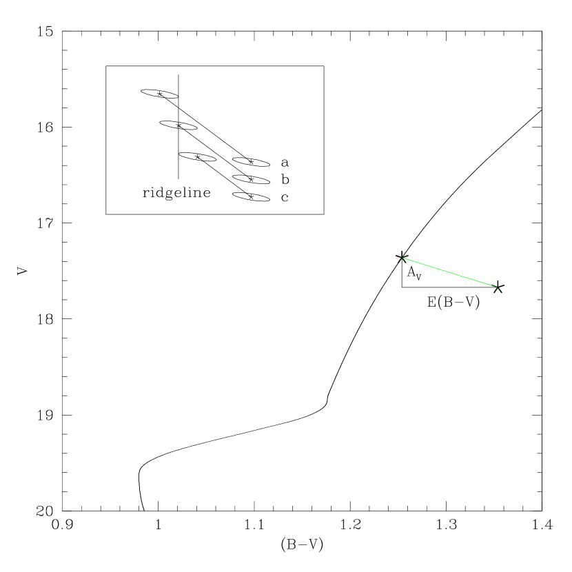
Figure 6: Example of how we move one of M 62’s star along the reddening vector (in green) until it intersect the ridgeline. From there a value for the color excess E(B-V) is obtained. In the upper left box, we schematically show how the error ellipse moves and how the error in the shift is calculated. The ’point of last contact’ of the error ellipse with the ridgeline is represented in a, the shift of the original datapoint until it intersects the ridgeline is represented in b, and the ’point of first contact’ of the error ellipse with the ridgeline is represented in c.

To calculate an extinction for every star we move the stars along the reddening vector until they intersect the ridgeline at an astrophysically reasonable location (see figure 6). The reddening vectors are described by the equations

$$A_{V}/E(B-V)=3.317$$ (22)

and

$$A_{V}/E(V-I)=2.411$$ (23)

as given in Schlegel et al. (1998), which are evaluated using the $R_{V}=3.1$ extinction laws of Cardelli et al. (1989) and O’Donnell (1994).

The HB ridgeline, and therefore also stars in the range $m_{HB}-m_{HBthickness}<m<m_{HB}+m_{HBthickness}$, are not used in this calculation, since we want to use them as an independent test of the accuracy of our method (see section 2.4). We do not use stars dimmer than the completeness limit defined in section 2.1 either. These stars and stars that do not intersect with the ridgeline are given a weight 0 in the calculation of the extinction map described in next section.

To calculate the error of these shifts we follow the analysis in von Braun & Mateo (2001):

• We created an error ellipse for every star defined by the Poisson error in its color, ${\sigma}_{c}$, and magnitude, ${\sigma}_{m}$.

• Since the color and magnitude errors are correlated, the error ellipse is tilted. The tilt angle and the length of the semi-major and semi-minor axes of the error ellipse are functions of the error in color and in magnitude.

  $$\tan(2{\theta})=\frac{2{\sigma}_{cm}}{{\sigma}^{2}_{c}+{\sigma}^{2}_{m}}$$ (24)

  $${\sigma}^{2}_{c^{\prime}}=\frac{{\sigma}^{2}_{c}+{\sigma}^{2}_{m}}{2}+\left[\frac{({\sigma}^{2}_{c}-{\sigma}^{2}_{m})^{2}}{4}+{\sigma}^{2}_{cm}\right]^{1/2}$$ (25)

  $${\sigma}^{2}_{m^{\prime}}=\frac{{\sigma}^{2}_{c}+{\sigma}^{2}_{m}}{2}-\left[\frac{({\sigma}^{2}_{c}-{\sigma}^{2}_{m})^{2}}{4}+{\sigma}^{2}_{cm}\right]^{1/2}$$ (26)

  where ${\theta}$ is the tilt angle of the error ellipse, ${\sigma}_{c^{\prime}}$ and ${\sigma}_{m^{\prime}}$ are the semi-major and semi-minor axis of the tilted ellipse, and ${\sigma}_{cm}$ is the covariance of the color and magnitude.

• For every star, we move the error ellipse along the reddening vector. The point of first contact (pfc), i.e., the point where the ellipse touches the ridgeline for the first time, and the point of last contact (plc), where the ellipse touches the ridgeline for the last time, represent the one-sigma-deviation points (see figure 6).

• Although these two contact points are not necessarily symmetric about the reddening value of the star, i.e., the center of the error ellipse, we are going to define the error in the shift as:

  $${\sigma}_{ellipse}=0.5(pfc+plc)-center$$ (27)

2.4 Creating the extinction map

We now take all the color excesses for the individual stars and smooth them using locfit to build a bivariate non-parametric regression of the extinction as a function of the spatial coordinates right ascension and declination, up to a distance from the center of the cluster equal to where $P(X=1|r)=0.1$ or the limit of our observations, whichever comes first (see table 3). This limit is adopted after preliminary application of our method to the clusters in our sample with looser restrictions, and not observing an improvement in the dereddened CMDs (see section 2.5) for stars located beyond these ranges. Stars that were given zero weight in the previous subsections (stars in the HB region, stars dimmer than the completeness limit, stars that do not intersect with the ridgeline after being moved along the reddening vector) are not taken into account for the calculation of the map, although after the map is built a reddening correction is applied to all of them. Preliminary weights are assigned in locfit to all stars as they were calculated in previous subsections, but now $w_{ph}=1/{\sigma}_{ellipse}^{2}$. The spatial smoothing kernel in this case has a constant bandwidth of $0.5^{\prime}\times 0.5^{\prime}$ or a nearest neighbor ratio of 0.03, whichever is bigger. These values for the smoothing parameter are used after experimentally checking in a few of our clusters which kernel provides us with a tighter HB, in the sense of a smaller standard deviation of the stars from the ridgeline of this region (see section 2.2), after generating the dereddened CMD (see section 2.5). This is an independent test to assess the quality of our dereddening method, since our technique does not use stars in the HB to calculate the extinction map. The tests gave similar results for a range of parameters. Since the tests were not highly conclusive on choosing a particular set of parameters, the set used is an average of the best values obtained for the different clusters tested.

Along with the extinction map, an extinction precision map is also calculated. This is done assuming that the precision of the extinction map is a function of the spatial coordinates. Hence, we can write

$$Y_{i}=r(\alpha_{i},\delta_{i})+\sigma(\alpha_{i},\delta_{i})\epsilon_{i},\ \mathbb{E}(\epsilon_{i})=0,\ \mathbb{V}(\epsilon_{i})=1$$ (28)

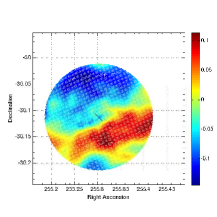
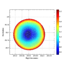
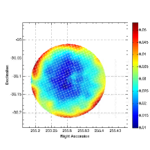
Figure 7: Extinction map for the M 62 cluster (left), along with its resolution (middle), and its precision (right), as provided by our technique. The x marks the position of the center of the cluster. The color code gives the color excesses $E(B-V)$ for the extinction map, the bandwidths used in the resolution map, and the standard deviation $\sigma$ of the color excesses in the precision maps. Notice that the adopted reddening zero point is defined by where our ridgeline lies, and has to be established from other methods (see text).

where $Y_{i}$ is the calculated extinction for the $i$-th star and $r(\alpha_{i},\delta_{i})$ is the value for the extinction provided by the regression function at the coordinates $(\alpha,\delta)$ of the $i$-th star. Therefore, regressing directly the square residuals $(Y_{i}-r(\alpha_{i},\delta_{i}))^{2}$ provides us with an estimate $\hat{\sigma}^{2}(\alpha_{i},\delta_{i})$ of the variance, and its square root allows us to plot a map of the standard deviation $\hat{\sigma}$ as a function of the spatial coordinates. This precision map provides us with a tool to improve our extinction map. We iteratively repeat the whole process of the calculation of extinction maps, but every time using only stars that have extinctions that are no more than $3\sigma$ away from the value that our previous extinction map gives for those coordinates. Preliminary weights and smoothing parameters are the same in every calculation. We repeat the process until it converges, i.e., until the number of stars used in the calculation of the extinction maps changes by less than $1\%$ with respect to the previous iteration. This way for every cluster we are able to provide an extinction map (see top plot of figure 7), a precision map for this extinction map (see bottom plot of figure 7), and a resolution map with the bandwidth that we have use in a certain region to calculate the extinction map there (see central plot of figure 7).

2.5 Creating the dereddened CMD

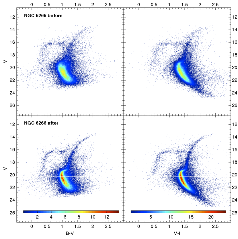
Figure 8: $B-V$ vs. $V$ (left) and $V-I$ vs. $V$ (right) CMDs of M 62, before and after applying our dereddening technique to them. Color bars show the range in the densities of stars in the CMD ($\times 10^{4}$ stars per square magnitude).

All the observed stars are given a reddening correction from the extinction map and a dereddened CMD is constructed (see figure 8). This dereddened photometry is the input on the next iteration to calculate the cluster membership probabilities, and to build a new improved ridgeline (see figure 1). Notice though that the input on the calculation of the individual reddenings to generate the extinction maps is the original photometry in every iteration (see figure 1).

We iteratively repeat this process until there is a convergence in the calculated ridgeline (see figure 1), which results in good convergence of the reddening values of the extinction map. For our dataset, convergence usually occurs after just two or three iterations.

3 Example: Dereddening M62

The method will be extensively applied to a sample of 25 globular clusters in following papers. Here, as an example, we applied the method to one of those clusters, M62.

M 62 (NGC 6266) is a moderately reddened, $E(B-V)=0.47$ cluster, located only $1.7kpc$ from the Galactic center (Harris, 1996), with a patchy extinction (Contreras et al., 2005, 2010). The observation, reduction and calibration processes will be explain in detail in Paper II. Suffice it to say here that $B$, $V$, and $I$ data for this cluster where obtained with the IMACS camera in the Magellan 6.5m telescope, and, in $V$ and $I$ for the inner part of the cluster with the WFPC2 camera on the HST. After applying fairly standard reduction and calibration processes to these data, we merged the databases from the two telescopes to obtain accurate astrometry (${\sigma}\sim 0.25^{\prime\prime}$ dispersion) and accurate photometry (${\sigma}\sim 0.2$ magnitude dispersion) in B,V and I for the stars in a field of $15^{\prime}\times 15^{\prime}$ centered in the cluster. In figure 8 we can see the resulting CMDs of this cluster.

The first step of our dereddening method is to calculate the probabilities $P(X=1|r,c,m)$ for the observed stars to belong to the cluster. To do that, we use the probability densities of the stars as functions of distance to the center of the cluster and of color and magnitude, a King profile plus constant field model, and a Besançon model for the field, as explained in section 2.1 (see figures 2, 3, and 4). The different parameters used to build the King and Besançon models for this calculation are shown in tables 1 and 2. Notice that we restrict our analysis to stars in the limits shown in table 3, because of the reasons mentioned in the previous sections.

Once the probabilities to belong to the cluster have been calculated, we need to build the ridgeline. Following the the three step recipe explained in section 2.2, we get the ridgelines in the two available colors (see figure 5). After that, we move the stars along the reddening vector until they intersect the ridgeline (see figure 6) and smooth the resulting individual color excesses, as explained in sections 2.3 and 2.4. We obtain the extinction map shown in figure 7. From this map, we take the relative extinction that corresponds to every star observed. We then plot the CMD of the stars in our observation after having been corrected for the differential reddening and use it as the input for the next iteration. The process converges for both colors after 3 iterations and we generate the dereddened CMDs that we can see in figure 8.

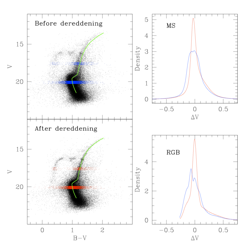
Figure 9: Distribution of stars in the $B-V$ color around the calculated ridgeline for two different magnitude cuts (1.5 mag above and 0.5 mag below the TO) for the stars in M 62, before (blue) and after (red) differentially deredden the CMD. The FWHM of the density distributions at the two magnitude cuts narrows by more than a factor of 2 after we have differentially dereddened the CMD (for the MS cut, $FWHM=0.262$ mag before and $FWHM=0.115$ mag after; for the RGB cut, $FWHM=0.267$ mag before and $FWHM=0.103$ mag after). The profiles also look more unimodal.

We leave the detailed examination and analysis of the physical characteristics of the cluster to Paper III, but we mention here how much better the definition of the different parts of the cluster is. The width of the MS narrows by a factor of 2 after being dereddened (see figure 9). This improvement will help us to obtain better constraints on the cluster age and distance when compared to theoretical isochrone models. The RGB is also narrowed by a factor of 2 (see figure 9), which will help when trying to better constrain the metallicities.

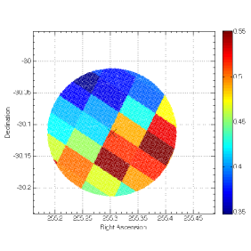
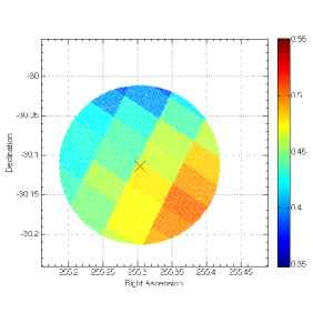
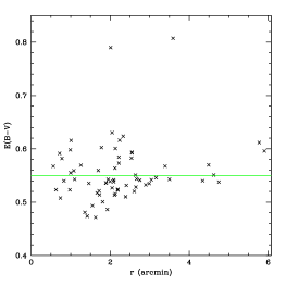
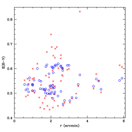
Figure 10: On top, comparison of the extinction map provided by our technique (left) with the extinction map created from the dust temperature maps by Schlegel et al. (1998) (right). We have degraded the resolution of our map to make it equal to the Schlegel map. We have found an extinction zero point offset between both maps of $E(B-V)=0.47$, that we have added to our map. On the bottom, comparison between the extinction values provided by Contreras et al. (2010) from the analysis a set of RRLyrae, and the extinction values at the same positions provided by our map: on the left, the substraction of both sets of extinction values allows to find the extinction zero point for our map, $E(B-V)=0.55$, as the weighted average of the substracted values (green line); on the right, comparisons of both sets of values (Contreras et al. (2010), as red crosses; this paper, as blue circles, after adding the extinction zero point).

As a reference, we compare the final reddening map obtained using our technique with maps and extinction values within the covered region available in the literature (see figure 10). We found a general agreement in the identification of regions of high and low extinction, although our map shows sharper features than the one presented by Schlegel et al. (1998), perhaps the result of their mapping the interstellar extinction in the foreground and also in the background of the cluster (upper plots in figure 10), and smoother values than those by Contreras et al. (2010), result of our spatial smoothing of the extinction values (lower plots in figure 10). As we have already mentioned, the technique explained in the paper does not calculate the absolute extinction toward a target cluster. Comparisons like the ones shown in figure 10 will allow to find the extinction of the adopted reddening zero point in our dereddening method.

Appendix A Non-parametric analysis using locfit

In our work we have extensively used non-parametric statistics to estimate probability density and regression functions directly, without reference to a specific form. This differs from other approaches in which probability density and regression functions are expressed in a parametric way, where the function used to describe them can be written as a mathematical formula which is fully described by a finite set of parameters that we have to find.

In our analysis we have used locfit, a local likelihood estimation software implemented in the R statistical programming language. Locfit is extensively explained in Loader (1999), so here we just want to give a general idea of how it works and the main tuning parameters that we have chosen in our analysis. Locfit does not constrain the functions globally, i.e., it is non-parametric, but assumes that locally, around a certain point x, the function can be well approximated by a member of a simple class of parametric functions. Locfit defines a local window around a point, weighting the observations according to their distance to that point

$$w_{i}(x)=\left\{\begin{array}[]{rcl}W(\frac{x_{i}-x}{h(x)})&\mbox{if}&x_{i}<|x+h(x)|\\ 0&\mbox{if}&x_{i}\geq|x+h(x)|\end{array}\right.$$

and inside this local window, the function is approximated by a polynomial, using not the usual local least square criterion but a local log likelihood criterion. We have to choose the weighting function and the order of the polynomial. For both cases we take the default given by the program: a polynomial of order 2 with a tricube weight function $W(u)=(1-|u|^{3})^{3}$. Still we are left with one last argument to choose, the smoothing parameter that controls the bandwidth $h(x)$. This smoothing parameter is defined by the maximum of two elements: a bandwidth generated by a nearest neighbor fraction $0<{\alpha}<1$, and a constant bandwidth. The nearest neighbor bandwidth is computed in two steps, first computing the distances $d(x,x_{i})=|x-x_{i}|$ for all the data points and then choosing $h(x)$ to be the kth smallest distance, where $k=[n{\alpha}]$.

Also the likelihood criterion can be chosen, and we choose for the regression the family qrgauss, which is equivalent to a local robust least squares criterion where outliers are iteratively identified and downweighted, similar to the lowess method (Cleveland, 1979).

If we want to give more weight to some points than others, locfit allows preliminary weights to be given to all observations.

A scale factor can be applied to the different variables in multivariate fitting, when variables are measured in non-comparable units, or when we want to give more importance to one of them like in the determination of the densities of stars in our CMD, where the range in color for the stars is smaller than the range in magnitudes.

In addition to calculating the non-parametric function that fits the data, locfit can also calculate the derivative of that function.

Finally, a word is in order about the evaluation structures in locfit. Locfit does not perform local regression directly in every point, but selects a set of evaluation points obtaining the fit there and interpolating later elsewhere. This is done for efficiency: it is much faster to evaluate the structure in a small number of points and then interpolate for the rest. But we should make sure that we do not lose information on the process. In order to achieve this, locfit uses, by default, a growing adaptive tree, which is the evaluation structure that we use in our analysis. A growing adaptive tree is a grid of points. One begins by bounding the data in a rectangular box and evaluating the fit at the vertices of the box. One then recursively splits the box into two pieces, then each subbox into two pieces and so on. For this kind of structure, an edge is always split at the midpoint and the decision to split an edge is based solely on the bandwidths at the two ends of the edge, depending on the score ${\delta}_{ij}=d_{ij}/min(h_{i},h_{j})$ where $d_{ij}$ is the distance between the two vertices of an edge, and $h_{i}$ and $h_{j}$ are the bandwidths used at the vertices. Any edge whose score exceeds a critical value c ($c=0.8$ by default) is split.

Table 1: Summary of the parameters used to obtain and fit the King models for M62

Core radius (according to most updated Harris catalog)	0.18 arcmin
Tidal radius (according to most updated Harris catalog)	8.97 arcmin
$k$ constant from the King profile (see $eq.\ 11$)	12264.7 stars arcmin-2
Surface density of non-member field stars from the fit (see $eq.\ 11$)	226.4 stars arcmin-2
Surface density of non-member field stars according to Besançon model	216.6 stars arcmin-2

Table 2: Summary of the parameters used to obtain the Besançon model for the non-cluster stars in the M62 region.

Field of view
Field	Small field
	l=$353.57^{\circ}$; b=$7.32^{\circ}$
	Solid angle=0.190 square degree
Extinction law
Diffuse extinction	0.0 mag/kpc
Discrete clouds	$A_{v}$=1.36; Distance=0pc
Selection on
Intervals of magnitude	$15.75\leq B\leq 25.14$
	$15.56\leq V\leq 23.71$
	$14.75\leq I\leq 22.44$
Photometric errors	Error function: Exponential
	Band=$B$; A=0.006, B=22.68, C=0.866
	Band=$V$; A=0.005, B=23.22, C=0.899
	Band=$I$; A=0.009, B=30.12, C=1.238

Table 3: Limits for the stars used in our analysis of M62

$V$ magnitude where the completeness limit is reached	21.51
$\Delta V$ between the completeness limit and the dimmest star in our ground observation	2.2
Distance where the ratio of GC stars to total number of stars drops to 0.1	6.20 arcmin

.

References

- Bedin et al. (2004) Bedin, L. R., Piotto, G., Anderson, J., Cassisi, S., King, I. R., Momany, Y., & Carraro, G. 2004 ApJ, 605, L125
- Calamida et al. (2005) Calamida, A., et al. 2005, ApJ, 634, 69
- Cardelli et al. (1989) Cardelli, J. A., Clayton, G. C. & Mathis, J. S. 1989, ApJ, 345, 245
- Cleveland (1979) Cleveland, W. S. 1979, J. Amer. Statist. Assn., 74, 829
- Contreras et al. (2005) Contreras, R., Catelan, M., Smith, H. A., Pritzl, B. J., & Borissova, J. 2005, ApJ, 623, L117
- Contreras et al. (2010) Contreras, R., Catelan, M., Smith, H. A., Pritzl, B. J., Borissova, J. & Kuehn, C. A. 2010, AJ, 140, 1766
- D’Antona & Caloi (2008) D’Antona, F., & Caloi, V. 2008, MNRAS, 390, 693
- Grillmair et al. (1995) Grillmair, C. J., Freeman, K. C., Irwin, M., & Quinn, P. J. 1995, AJ, 109, 2553
- Harris (1996) Harris, W. E. 1996, AJ, 112, 1487
- Heitsch & Richtler (1999) Heitsch, F., & Richtler, T. 1999, A&A, 347, 455
- Hughes & Wallerstein (2000) Hughes, J., & Wallerstein, G. 2000, AJ, 119, 1225
- Hughes et al. (2007) Hughes, J., Wallerstein, G., Covarrubias, R., & Hays, N. 2007, AJ, 134, 229
- Kaluzny & Krzeminski (1993) Kaluzny, J., & Krzeminski, W. 1993, MNRAS, 264, 785
- King (1962) King, I. 1962, AJ, 67, 471
- Law et al. (2003) Law, D. R., Majewski, S. R., Skrutskie, M. F., Carpenter, J. M., & Ayub, H. F. 2003, AJ, 126, 1871
- Loader (1999) Loader, C. 1999, Local Regression and Likelihood, (New York: Springer)
- Marín-Franch et al. (2009) Marín-Franch, A., et al. 2009, ApJ, 694, 1498
- Melbourne & Guhathakurta (2004) Melbourne, J. & Guhathakurta, P. 2004, AJ, 128, 271
- Mighell et al. (1998) Mighell, K. J., Sarajedini, A., & French, R. S. 1998, AJ, 116,2395
- Odenkirchen et al. (2001) Odenkirchen, M., et al. 2001, ApJ, 548, 165
- O’Donnell (1994) O’Donnell, J. E. 1994, ApJ, 422, 1580
- Piersimoni et al. (2002) Piersimoni, A. M., Bono, G., & Ripepi, V. 2002, AJ, 124, 1528
- Piotto et al. (1999a) Piotto, G., Zoccali, M., King, I. R., Djorgovski, S. G., Sosin, C., Dorman, B., Rich, R. M. & Meylan, G. 1999, AJ, 117, 264
- Piotto et al. (1999b) Piotto, G., Zoccali, M., King, I. R., Djorgovski, S. G., Sosin, C., Rich, R. M. & Meylan, G. 1999, AJ, 118, 1727
- Piotto et al. (2007) Piotto, G., Bedin, L. R., Anderson, J., King, I. R., Cassisi, S., Milone, A. P., Villanova, S., Pietrinferni, A., & Renzini, A. 2007, ApJ, 661, L53
- Robin et al. (2003) Robin, A. C., Reylé, C., Derrière, S., & Picaud, S. 2003, A&A, 409, 523
- Schechter et al. (1993) Schechter, P., Mateo, M., & Saha, A. 1993, PASP, 105, 1342
- Schlegel et al. (1998) Schlegel, D., Finkbeiner, D., & Davis, M. 1998, ApJ, 500, 525
- Valenti et al. (2007) Valenti, E., Ferraro, F. R., & Origlia, L. 2007, AJ, 133, 1287
- von Braun & Mateo (2001) von Braun, K. & Mateo, M. 2001 AJ, 121, 1522