Forward-Backward Correlations and Event Shapes as probes of Minimum-Bias Event Properties

Abstract

Measurements of inclusive observables, such as particle multiplicities and momentum spectra, have already delivered important information on soft-inclusive (“minimum-bias”) physics at the Large Hadron Collider. In order to gain a more complete understanding, however, it is necessary to include also observables that probe the structure of the studied events. We argue that forward-backward (FB) correlations and event-shape observables may be particulary useful first steps in this respect. We study the sensitivity of several different types of FB correlations and two event shape variables — transverse thrust and transverse thrust minor — to various sources of theoretical uncertainty: multiple parton interactions, parton showers, colour (re)connections, and hadronization. The power of each observable to furnish constraints on Monte Carlo models is illustrated by including comparisons between several recent, and qualitatively different, Pythia 6 tunes, for $pp$ collisions at $\sqrt{s}=900\,$GeV.

1 Introduction

Until recently, the measurements used to constrain physics models of high energy particle collisions came primarily from experiments done at the previous generations of accelerators, such as the SPS, LEP, and the Tevatron. In particular, studies of “minimum-bias” and underlying-event physics have been widely used to constrain the poorly known non-factorizable and non-perturbative aspects of Monte Carlo (MC) event generators. These generators are, in turn, used ubiquitously over a continually expanding range of energies and intensities, for both high- and low-$p_{\perp}$  processes. MC “tunes” that rely exclusively on these older data sets are, however, becoming outmoded by a new generation of high-energy experiments, performed at the Large Hadron Collider (LHC). The extrapolation of previous results to the higher energies and large acceptances of the LHC experiments is associated with significant uncertainties, and the demands on both theoretical and experimental precision are becoming ever more stringent. The importance of reevaluating the physics models, and of retuning them in situ, has therefore been highlighted in several recent studies Buttar:2008jx ; atlasmc09 ; Skands:2010ak ; Butterworth:2010ym ; Abdesselam:2010pt ; Deak:2010gk ; Aad:2010fh .

The LHC offers a rich cornucopia of opportunities to test and expand the data sets used for MC tuning. Moving from the low-$p_{\perp}$ results of minimum-bias to the underlying event in hard processes, and from central rapidities to ones close to the beam axis, we may test the universality and applicability of the modeling over a large dynamical range.

For minimum bias (MB), which is the focus of this paper, there is no “hard scale”, and hence all observables receive large non-perturbative corrections. From the point of view of a theoretical modeling based on factorization and perturbative QCD, it is difficult to say anything meaningful about this data set, except perhaps for the tiny fraction of it that includes hard jets. In Pythia, as in most other contemporary MC models, the modeling of soft-inclusive physics, is based on the concept of Multiple Parton Interactions (MPI). Though these corrections go beyond the reach of the standard factorization theorems, they are still regarded as essentially perturbative in origin; they are dominated by (multiple) $t$-channel gluon exchanges, regulated by a non-perturbative dampening at low $p_{\perp}$, and dressed with non-perturbative descriptions of the beam remnants and of the hadronization process. We shall not here go into the details of the modeling (for a recent review, see Buckley:2011ms ). It is worth noting, however, that the smooth transition between soft and hard scattering processes is the main reason the Pythia modeling can be used for both minimum-bias and underlying-event physics. As mentioned above, this universality is important, since by testing the model in a minimum-bias environment here, we may expect to simultaneously improve the description also of other physical processes.

Particle multiplicities and transverse momentum spectra are generally used to give the first important constraints on the overall amount of particle production and on its distribution in $p_{\perp}{}$ and $\eta$. Several such studies have already been published by the LHC collaborations Khachatryan:2010xs ; Aad:2010rd ; Aamodt:2010pp ; Aamodt:2010ft ; Khachatryan:2010us ; Aamodt:2010my ; Khachatryan:2010nk ; Collaboration:2010ir ; ref:MB20 . However, as most people familiar with MC tuning will be aware of, there are often several qualitatively different ways of mixing the same cocktails. (I.e., several tune parameter sets may reproduce the same experimental data.) An important question therefore concerns the balance between the several different particle production mechanisms that are available to an open-minded model builder: initial- and final-state radiation, beam remnant breakup, “hard” processes vs. additional MPI interactions, final-state interactions, etc. Each production mechanism generally has some kinematical or dynamical “signature” that can be used to single it out, if sufficiently differential information is available. Tests using several, mutually complementary, discriminating observables are therefore to be regarded as essential to overcome model degeneracies.

In the context of the present paper, it is especially important to note that the collinear enhancements characteristic of parton shower activity tend to produce local / short-range correlations, i.e., the additional particle production caused by the showering dies away rather quickly with distance to the originating parton. By contrast, the particle production associated with semi-hard MPI (mini-)jets tends to produce an enhancement of correlations around $\Delta\phi=\pi$ while soft particle production from strings stretched between the remnants should generate long-range correlations in rapidity which, to a first approximation, should be homogeneous in $\phi$. Thus, the shape of events and the particle-particle correlations within them, can be used to gain a handle on the relative strengths of different particle production mechanisms.

In section 2, we briefly present the Monte Carlo models we shall use, and discuss the various sources of particle production relevant to soft-inclusive physics. A mild selection bias is then introduced in section 3, to mimic a “minimal” minimum-bias selection, and the effect of including additional $p_{\perp}$ cuts is illustrated. In section 4, we briefly compare our reference models on some of the typical minimum-bias plots, such as charged multiplicity, $\eta$, and $p_{\perp}$ distributions. In section 5, we then turn to a more detailed study of forward-backward correlations, including ones with an explicit $\phi$ dependence, and in section 6 we discuss the transverse thrust and the transverse minor. We give concluding remarks in section 7.

2 Monte Carlo Models and Parameters

For details on the modeling of hadron collisions incorporated in general-purpose event generators, we refer the reader to the recent review Buckley:2011ms . Here, we use the Pythia 6 generator throughout and focus on a few main aspects of the modeling that it will be useful for the reader to be aware of.

Firstly, the modeling of the diffractive contribution to soft-inclusive processes in Pythia 6 is somewhat crude. It uses parametrized cross sections to predict the rates of single (SD) and double (DD) diffractive dissociation differentially in the mass(es) of the diffracted system(s) Sjostrand:2006za . Each diffractively excited system is represented by a single “string” of the given mass, which is hadronized according to the Lund string fragmentation model Andersson:1983ia ; Andersson:1998tv . We note that this type of diffractive modeling can be characterized as “soft” since it does not include a mechanism for hard, high-mass diffraction, such as diffractive jet production. We include it, nonetheless, to give an idea of how the bulk of soft diffractive processes affect our conclusions. We also note that “typical” minimum-bias cuts are designed to reduce the contamination by diffractive processes, such that our conclusions should not depend too crucially on the modeling of this component.

The modeling of inelastic, non-diffractive processes is more sophisticated and is based on a picture of multiple parton interactions (MPI). In Pythia 6, there are two basic MPI frameworks available, which we shall refer to as “old” Sjostrand:1987su and “new” Sjostrand:2004pf ; Sjostrand:2004ef . (The latter is similar to the modeling in Pythia 8.) Briefly stated, the main differences between the old and new models are:

• Old: virtuality-ordered parton showers, no showers off the additional MPI, and a relatively simple description of the fragmentation of the beam remnants in which the baryon number is carried by the remnant.

• New: transverse-momentum-ordered parton showers, including showers off the additional MPI, and a more sophisticated treatment of the beam remnant, in which “string junctions” Sjostrand:2002ip carry the beam baryon number.

In both cases, the fundamental MPI cross sections are derived from a Sudakov-like unitarization/resummation of perturbative QCD $2\to 2$ scattering Sjostrand:1987su , normalized to the total inelastic non-diffrative cross section, and regulated at low $p_{\perp}$ by a smooth dampening factor. The latter is interpreted as being due to colour screening, and the dampening scale, $p_{\perp 0}$, represents the main tunable parameter of the model. Two other significant parameters are the assumed transverse shape of the proton (lumpy or smooth), and the strength of colour reconnections (CR) in the final state, cf. Buckley:2011ms .

2.1 PYTHIA Tunes

We shall consider a small selection of recent tunes that use the “old” and “new” models, as follows. Field’s Tune DW Albrow:2006rt is currently the “preferred” Tevatron tune and has been extensively tested there. Perugia 0 Skands:2010ak also attempts to give a good fit to Tevatron data, but uses the new model and incorporates an updated set of fragmentation parameters tuned to LEP data by the Professor collaboration Buckley:2009bj . That collaboration’s own tunes of the old and new model are called Q20 and PT0, respectively Buckley:2009bj . Finally, we also include a tune called ACR Skands:2007zg , which represents a hybrid between the two models; it uses the basic shower and MPI framework from the old model with the colour-reconnection (CR) model of the new one. It is included to make it possible to isolate whether specific features are due only to the CR model or not. All tunes were run with Pythia version 6.4.21. Table 1 show the tunes used along with their three-digit codes in the Pythia subroutine PYTUNE,

Parameter	DW	ACR	Q20	P0	PT0
PYTUNE	103	107	129	320	329

Table 1: Pythia tunes and corresponding three-digit PYTUNE codes.

2.2 Sub-Process Samples

Pythia includes four distinct processes in its simulation of soft-inclusive physics: elastic scattering, single diffractive dissocation, double diffractive dissociation, and inelastic non-diffractive (low-$p_{\perp}$) interactions. The sum of these contributions is the total hadron-hadron cross section.

Elastic scattering occurs when the colliding protons interact without either of the beam hadrons breaking up. We shall not consider this source further, since it does not produce any particles at central rapidities.

In single diffractive dissociation (SD), one of the incoming hadrons breaks up, and the other does not. In this situation, a spread of low-$p_{\perp}$ particles is expected from the disintegrated system over a limited rapidity region near the dissociated hadron, while the undissociated one continues with a modified momentum.

Double diffractive dissociation (DD) involves the break-up of both beam particles. Here, both systems generate significant low-$p_{\perp}$ particle deposits from disintegration over rapidity, typically with a gap between them.

Low-$p_{\perp}$ or non-diffractive interaction involves partonic scattering processes, all the way from soft to hard, with the latter mapping smoothly onto the dijet tail. In this case particle production is more localized, with higher-$p_{\perp}$ constituents and the possibility — switched on by default — of additional perturbative activity such as parton showers and multiple parton interactions.

For all tunes, we start from an inclusive sample composed of the three inelastic process types, distributed according to their relative cross sections, which are fixed by Pythia’s default parametrizations ref:Pythia_man . Since the description of the diffractive components is quite simple, it would not make much sense to attempt to isolate individual contributions to the particle production within the two diffractive samples. The particle production in the low-$p_{\perp}$ sample, however, receives contributions from several different algorithmic components which we may label as: “hard” scattering, parton showers, MPI, and remnant fragmentation, each with its own distinct behaviour.

In order to isolate what happens as each component is “switched on”, we consider four different variants of the low-$p_{\perp}$ sample:

1. low-$p_{\perp}$: Everything on, corresponding to the most physical description of the low-$p_{\perp}$ sample.

2. HARD: No parton showers, no MPI. I.e., a single partonic $2\to 2$ interaction, with no parton showers.

3. RAD: No MPI. I.e., a single partonic $2\to 2$ interaction, with parton showers.

4. MPI: No parton showers. I.e, multiple parton-parton interactions, without showers.

Note that all variants are passed through the string fragmentation model in order to give final-state hadrons.

For each sample (and for each variation of the low-$p_{\perp}$ one), 100,000 $pp$ collisions were generated at $\sqrt{s}=900\,$GeV. This sample size is sufficient to overcome statistical fluctuations for the measurements of interest, and more than the data set in ref:UA5_b . Obviously, larger sample sizes would still be of interest, to study the tails of distributions, but we shall here mostly be concerned with the bulk of the physics.

3 Selection Procedure

Our starting point is a very loose selection, requiring at least some activity in a rather broad central region consistent with the charged-particle acceptance region of the UA5 experiment. Thus, only stable charged particles within a pseudo-rapidity range of $\eta=(-5.,5.)$ are selected. Although the central trackers of the ATLAS and CMS experiments only extend to pseudorapidities of $\pm 2.5$, we note that the Forward Multiplicity Detector (FMD) Christensen:2007yc in the ALICE experimented could be used to extend charged-particle measurements of the types we consider to include pseudorapidities up to $\eta\sim 5$. By stable charged particles, we mean all charged particles with proper lifetimes ${c\tau}>10\,\mathrm{mm}$ (thus, e.g., $\Lambda$ and $K$ hadrons are stable). By default, we do not apply any cuts in $p_{\perp}$ unless explicitly stated otherwise. Selected events must have at least one charged particle in the $\eta$-range.

Table 2 shows the percentages of selected events with this mild requirement. For elastic events, the corresponding percentage would be zero, as the scattered protons continue on “down the beam-pipe”, outside the range of selection. Of the included sub-processes, a significant fraction of SD events are rejected already at this point, as are about half that fraction of the events labeled DD. These correspond to events where the fragments of the dissociated proton(s) were concentrated at high rapidities, beyond the acceptance region. The events in the DD sample are less likely to be rejected, since they have two “chances” to produce particles in the central region. The low-$p_{\perp}$ ones are selected with approximately 100% efficiency. The “mix” sample contains the sum of all three subprocesses, weighted according to their respective cross sections as given by Pythia. The particle production samples (hard process only, radiative, MPI and combined i.e. low-$p_{\perp}$) have similar selection rates as they all include a central ‘hard’ interaction.

An illustration of the effect of the event selection on the inclusive $p_{\perp}$ distribution is shown in figure 1, for the low-$p_{\perp}$ sample. The top pane shows the $p_{\perp}$ distribution of all generated tracks in black and of the selected ones in green, for the DW tune. The main effect is a reduction in the total number of accepted tracks by 10-15%. A secondary effect, however, is a model-dependent hardening of the spectrum. We highlight this in the lower pane, which shows the ratio of selected to unselected tracks for each of the tunes. We observe that the DW and Q20 tunes of the “old” model exhibit an approximately constant value of this ratio, indicating that the shape of the $p_{\perp}$ spectrum is not greatly different at high rapidities than in the central region. By contrast, the tunes of the “new” model (P0 and PT0) exhibit a noticeable shape, indicating that for those models, the spectrum of the unselected high-rapidity tracks is systematically softer than in the central region. Also, since the hybrid ACR tune follows the “new” tunes here, we may interpret this behaviour as being related to the CR model used in the new tunes.

We note that these differences would translate directly to uncertainties for any purely model-based extrapolation beyond the central region. For the remainder of this report, however, we shall be concerned only with the central region itself.

	mix	SD	DD	low-$p_{t}$	HARD	RAD	MPI
DW	73%	70%	86%	100%	100%	100%	100%
ACR	73%	70%	86%	100%	100%	100%	100%
Q20	73%	69%	86%	100%	100%	100%	100%
P0	73%	68%	85%	100%	100%	100%	100%
PT0	73%	68%	85%	100%	100%	100%	100%

Table 2: Selection efficiencies for various Pythia sub-processes and particle production mechanisms for each tune. Each sample consisted of 100,000 generated events.

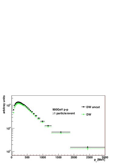
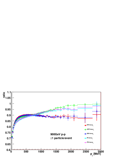
Figure 1: Above: Charged particle $p_{\perp}$ distribution for low-$p_{\perp}$ sample of DW tune, with (green) and without (black) $\eta$ selection cut. Below: Ratio of selected to unselected tracks for the low-$p_{\perp}$ sample of each tune.

4 Inclusive Distributions

Current LHC studies of minimum-bias events, e.g. Khachatryan:2010xs ; Aad:2010rd ; Aamodt:2010pp ; Aamodt:2010ft ; Khachatryan:2010us ; Aamodt:2010my ; Khachatryan:2010nk ; Collaboration:2010ir ; ref:MB20 , have focused mainly on the “basic four” charged-particle distributions: $P(n_{ch})$, $dn_{ch}/d\eta$, $dn_{ch}/dp_{t}$, and $\left<p_{t}\right>$ vs. $n_{ch}$. In this section, we comment briefly on these and illustrate the behaviour of our chosen set of Monte Carlo tunes for later reference. More comments on these distributions can be found, e.g., in Skands:2010ak ; Buckley:2011ms .

4.1 Multiplicity

In table 3, we compare the average charged particle multiplicity, $\left<n_{ch}\right>$, between tunes, for the three different inelastic samples, as well as for their cross-section-based mixture. At this point, we subject the samples only to the selection requirement $|\eta|\leq 5$ mentioned above. Table 4 contains an equivalent comparison, for the different physics variations of the low-$p_{\perp}$ sample. To help illustrate the overall spread in predictions, we also quote a “range” of variation, at the bottom of each table, which is defined as the highest average multiplicity of the tunes minus the lowest, normalized to the lowest multiplicity, i.e.

$$\mbox{range}=(\left<n_{ch}\right>_{\mathrm{max}}-\left<n_{ch}\right>_{\mathrm{min}})/\left<n_{ch}\right>_{\mathrm{min}}\leavevmode\nobreak\ .$$ (1)

The range of $\left<n_{ch}\right>$ predicted within $|\eta|\leq 5$ varies by 10–20% between the different tunes for each of the inelastic sub-processes in table 3. For the diffractive processes, there is no parton showering and no MPI. The considerable differences between models are therefore solely generated by the different tunings of the hadronization model. Since in particular Q20 and PT0 were tuned to exactly the same LEP data by exactly the same tuning program (Professor), the difference between them here highlights the need for in situ constraints on the non-perturbative fragmentation parameters. It also indicates the need for a Monte Carlo modeling of diffraction that would be more theoretically consistent with the treatment at LEP, where the fragmentation parameters are dependent, e.g. on the perturbative parton shower cutoff. For the time being, we conclude that the fragmentation tuning of the new model used by PT0 and P0 produces fewer particles in and of itself than that of the old models. This appears to be consistent with the $p_{\perp}$ distributions shown in 3; fewer particles produced from the same energy of collision will result in a larger proportion of high-$p_{\perp}$ particles in selected events. Though not the main focus of this report, this would clearly be worth a more detailed analysis especially in the context of diffractive studies.

Tune	SD	DD	low-$p_{\perp}$	mix
DW	10.1	12.0	38.6	23.5
ACR	10.1	12.0	38.4	23.5
Q20	10.3	12.1	38.3	23.4
P0	9.1	10.8	35.4	21.7
PT0	9.1	10.8	36.8	22.5
range in $\left<n_{ch}\right>$ (%)	14.1	12.8	9.0	8.5

Table 3: Average charged particle multiplicity for the various minimum-bias sub-processes and tunes.

Tune	HARD	RAD	MPI	All on
DW	28.0	32.9	33.5	38.6
ACR	-	31.6	36.2	38.4
Q20	29.1	30.9	36.3	38.3
P0	23.8	26.0	29.6	35.4
PT0	24.1	26.0	31.1	36.8
range in $\left<n_{ch}\right>$(%)	22.4	26.6	22.4	9.0

Table 4: Average charged particle number for each particle production mechanism. Note: the column labeled “All on” is identical to the “low-$p_{\perp}$” one in table 3.

4.2 Track $p_{\perp}$

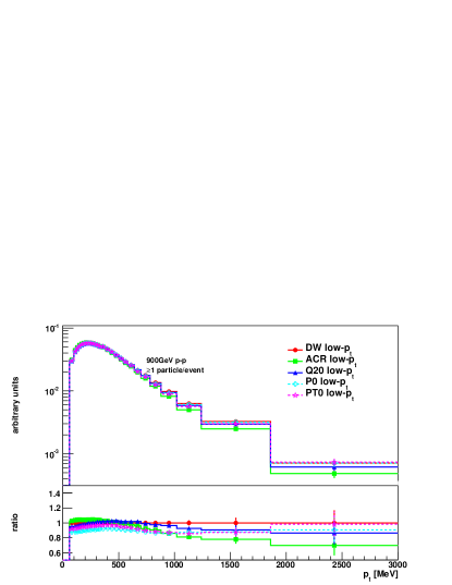
Figure 2: Selected charged particle logarithmic $p_{\perp}$ distribution for low-$p_{\perp}$ sub-sample Pythia tunes. Lower pane: ratio to the DW distribution.

Figure 2 shows the $p_{\perp}$ distributions for the low-$p_{\perp}$ sample of each tune, with the range of variation of the average $\left<p_{\perp}\right>$ spanned by the tunes for all the sub-samples given in table 5, with the range defined as in eq. (1).

As before, we note that the tunes exhibit differences of the order 10–20%. In the low region ($p_{\perp}<1\,\mathrm{GeV}$) the old shower tunes DW, ACR and Q20 lie above the new shower models P0 and PT0. This reverses in the region above $2\,\mathrm{GeV}$. Due to limited statistics, we do not plot the tail of very high-$p_{\perp}$ charged particles here, but note that the trend of the new models to generate harder $p_{\perp}$ tails is illustrated in Skands:2010ak .

	mix	SD	DD	low-$p_{t}$	HARD	RAD	MPI
range in $\left<p_{t}\right>$ (%)	5.7	3.1	3.5	6.1	10.5	6.1	10.5

Table 5: Range of mean $p_{t}$ values for various Pythia sub-processes and particle production mechanisms for each tune.

4.3 Track $\eta$

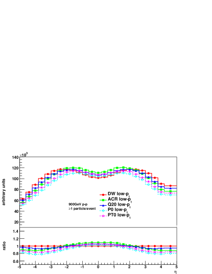
Figure 3: Selected charged particle logarithmic $\eta$ distribution for low-$p_{\perp}$ sub-sample Pythia tunes. Lower pane: ratio to the DW distribution.

Figure 3 shows the $\eta$ distributions for the selected models. Differences are again at the 10–20% level. Especially in the context of this distribution, such differences have sometimes been represented as “large”. Let us recall, however, that the Pythia modeling is rooted in perturbative QCD, that we are here dealing with processes which have no hard scale, and that the number of charged particles is not an infrared safe observable. In this light, while we might still hope to constrain the modeling better, we nonetheless wish to point out that it is, in our opinion, grossly misleading to characterize order 10% differences as large.

Indeed, the small differences between tunes are highlighted by the zero-suppressed Y-axis in the plot. Thus, while there is clearly some sensitivity to central vs. forward production mechanisms in this distribution, its ability to discriminate between models is still limited. Agreement between each tune is generally good, especially in the most easily observable region, $|\eta|<2.5$. We conclude that additional, linearly independent, information on the structure of events in $\eta$, could provide valuable additional constraints.

5 Forward-Backward Correlations

We come now to the main part of this report, in which we study several types of forward-backward correlations, $b$, for different production mechanisms, cuts, and correlation regions.

The purpose of these distributions is to enhance the discriminating power between models, and to reveal their properties more clearly, as compared to what can be achieved with the list of observables discussed in section 4. In particular, the collinear singularity structure of bremsstrahlung corrections in perturbative QCD causes initial- and final-state shower activity to generate strong but primarily short-range correlations, spanning at most a few rapidity units, whereas coloured exchanges between the beam hadrons (e.g., MPI) can generate correlations that are weaker but which span the entire rapidity range between the remnants. Thus, the shapes and normalizations of the $b$ distributions contain valuable information on the relative dominance of different particle production mechanisms, information which we argue is linearly independent from that contained in the current “standard” distributions.

This section is divided as follows: we first consider a standard inclusive “minimum-bias” $b$ correlation in section 5.1, illustrating how it is affected by different choices of bin size and by $p_{\perp}$ cuts; in section 5.2, we illustrate the sensitivity of this correlation to different particle production mechanisms, using the HARD, RAD, and MPI samples defined above, and to contamination by diffractive processes (SD, DD). In this way, we gain a map of how different cuts and different process mixtures affect the correlations, that we hope will be useful for future reference. We shall seek to extract further information by defining also a set of $b$ correlations that are sensitive to the azimuthal structure of the events, which will be the focus of section 5.3. We shall refer to these latter observables, which are essentially binned double-differential $\eta$-$\phi$ correlations, as “twisted” $b$ correlations.

5.1 Inclusive b Correlation

The standard $b$ correlation is defined as:

$$\centering b=\frac{\sigma(n_{b},n_{f})}{\sigma(n_{b})\sigma(n_{f})}=\frac{\left<n_{b}n_{f}\right>-\left<n_{f}\right>^{2}}{\left<n_{f}^{2}\right>-\left<n_{f}\right>^{2}}\leavevmode\nobreak\ ,\@add@centering$$ (2)

where $n_{f}$ ($n_{b}$) is the activity in a specific forward (backward) region of the detector. “Activity” can be measured by a number of observables in the detector, e.g., energy, charged particle multiplicity (inclusively or above a given $p_{\perp}$ threshold), momentum sum, etc. Here, we shall focus on the charged-particle multiplicity, as has also been done in most previous studies, though we emphasize that, e.g., calorimetric energy sums, could also be interesting to explore (see, e.g., Skands:2010ak ).

The “forward” and “backward” regions are defined by bins of a specific size in $\eta$ — typically chosen to be between 0.1 and 1.0 unit wide in $\eta$ — which are separated by some variable distance and arranged symmetrically around a midpoint which is usually taken to be the centre of the detector, $\eta_{c}=0$, corresponding to the CM of the colliding hadrons. Although we shall not do so here, we note that correlations between the central and forward region are also of interest and can be probed, for example, by fixing one bin in the central region and letting the other slide into the forward or backward region, corresponding to choosing $\eta_{c}\neq 0$. A study somewhat along these latter lines has been performed by UA5 ref:UA5_b and could also be interesting to maximize usage of the asymmetric coverage of the ALICE FMD.

The optimum bin size to use in eqn. (2) is a function of statistics and of the $\eta$-range observed. If the bin size is too small, genuine correlations will be washed out by statistical fluctuations. With too large a bin size, the resolving power of the correlation over the limited $\eta$-range will be lost.

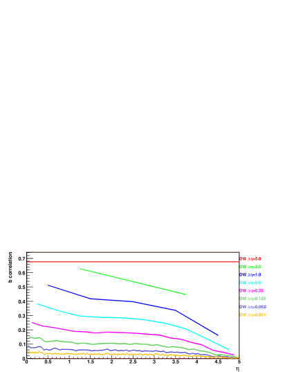
Figure 4: $b$ correlation for selected events with various pseudo-rapidity bin sizes, $\Delta\eta$. The single-point correlation for a bin size of $\Delta\eta$=5.0 (red) is shown covering the whole $\eta$-region.

Figure 4 contains a comparison of the $b$ correlation vs. $\eta$ (specifically the $\eta$ value of the centre of the forward bin, with the backward one located at $-\eta$) for varying bin sizes from 0.03 to 5 units wide, without imposing any $p_{\perp}$ cuts at this point. Obviously, the largest sizes are too coarse to discern much structure in the correlation distribution. Mid-range bin sizes, $\Delta\eta$=1.0, 0.5 and 0.25 exhibit best the trends over the $\eta$-range; for this particular model (DW), a high correlation at low $\eta$ can be distinguished from a mid-$\eta$ plateau and a further drop in correlation at high $\eta$. Going to even smaller bin sizes, $\Delta\eta$=0.125, 0.0625 and 0.03125, we begin to lose the structure in the distribution as statistical fluctuations start to dominate. We conclude that a bin size of $\Delta\eta$=0.5 is reasonable for this study. Note, however, that going to different CM energies and/or imposing $p_{\perp}$ cuts could change this conclusion; the average accepted multiplicity at each $\eta$ value determines the relative size of the statistical fluctuations and hence affects the optimum bin size. As a consequence, it is not possible, therefore, to directly compare $b$ distributions taken with different cuts, or which use different-sized $\Delta\eta$ bins.

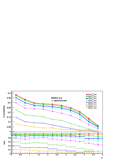
Figure 5: The $b$ correlation distributions for hadron-level charged particles for the DW tune with various explicit $p_{\perp}$ cuts. Lower pane: ratio to the non-cut distribution.

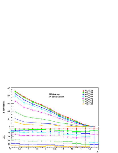
Figure 6: The $b$ correlation distributions for hadron-level charged particles for the Perugia 0 tune with various explicit $p_{\perp}$ cuts. Lower pane: ratio to the non-cut distribution.

To illustrate the effect of $p_{\perp}$ cuts, figs. 5 and 6 show the $b$ correlations subjected to a range of different $p_{\perp}$  cuts for a tune of the old (DW) and new (Perugia 0) model, respectively. (Note that these cuts are applied also at the level of the event selection, so only events with at least one particle harder than the given $p_{\perp}$ cut are included, for each curve.) One clearly sees the reduction of the correlation strengths as fewer tracks make it into each bin. Note that only positive correlations are expected and plotted. We interpret any small negative correlations as arising from statistical fluctuations in poorly populated bins.

	central bin			mid-range bin			extreme bin
Tune	$b_{0}$	$b_{0.5}/b_{0}$	$b_{1.5}/b_{0}$	$b_{0}$	$b_{0.5}/b_{0}$	$b_{1.5}/b_{0}$	$b_{0}$	$b_{0.5}/b_{0}$	$b_{1.5}/b_{0}$
DW	0.38	0.79	0.39	0.28	0.74	0.24	0.06	0.46	-0.08
ACR	0.45	0.71	0.34	0.28	0.68	0.30	0.05	0.38	-0.03
Q20	0.43	0.74	0.29	0.27	0.68	0.17	0.05	0.42	0.16
P0	0.46	0.72	0.23	0.23	0.66	0.18	0.00	0.71	-0.39
PT0	0.45	0.73	0.23	0.24	0.65	0.18	0.01	0.15	-0.05

Table 6: Central($\eta$=0-0.5), mid-range ($\eta$=2.5-3) and extreme ($\eta$=4.5-5) correlation values with fraction of correlation remaining after $p_{\perp}$-cut= 0.5GeV and 1.5 GeV for various Pythia tunes at $\sqrt{s}$=900GeV. $b_{0}$ is the correlation value for $p_{\perp}$-cut=0.0GeV, $b_{0.5}$ the value with $p_{\perp}$-cut=0.5GeV and $b_{1.5}$ the value $p_{\perp}$-cut=1.5GeV.

Table 6 summarizes the effect of $p_{\perp}$ cuts by giving the $b$ correlation values in the central ($|\eta|$=0-0.5), mid-range ($|\eta|$=2.5-3) and extreme ($|\eta|$=4.5-5) bins, without any $p_{\perp}$ cut, together with the reduction in the correlation strengths caused by $p_{\perp}$ cuts of $500\,$MeV and $1.5\,$GeV. In the central $\eta$-region, the effect of the $p_{\perp}=500\,$MeV cut (pink dashed line in figs. 5 and 6) is to lower the correlation by 20 – 30%. When the $p_{\perp}$ cut is increased to 1.5 GeV (dark purple solid line, second from bottom in the plots), the reduction is much more severe, and more interestingly is not a simple scaling from the reduction caused by the previous cut. Thus, e.g., ACR exhibits the largest reduction with the first cut, but the second-to-least with the second. Also interestingly, this pattern changes as one goes from mid-range to the extreme $\eta$ bins. (At the extreme end, though, the correlations are small, especially with high-$p_{\perp}$ cuts, and hence are easily overpowered by statistical fluctuations.) When comparing correlation values surviving the 500 MeV cut between central and extreme $\eta$-bins, we may conclude that the particle momentum distributions are heterogeneous across the $\eta$-range, due to the different parameters between tunes and differing particle production mechanisms. Measurements should therefore by no means be restricted to the most inclusive definition possible for a given experiment.

As a final summary of this part of the study, fig. 7 contains a comparison of the $b$ correlation distribution for each of the different tunes, again without $p_{\perp}$ cuts imposed. As was already apparent from figs. 5 and 6, the old and new models exhibit qualitatively different shapes. We interpret this in the following way: due to the inclusion of showers off the MPI in the new models, more of their total particle production is driven by shower activity than what was the case in the old ones, which have a larger average number of MPI Skands:2010ak . The new models therefore exhibit stronger short-range correlations and weaker long-range ones than their older counterparts, with a crossover point somewhere around $|\eta|=1-2$.

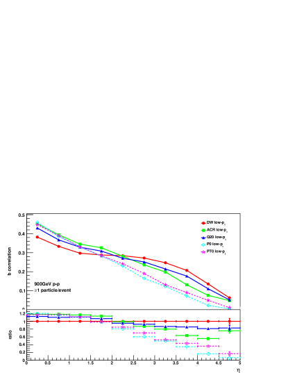
Figure 7: Inclusive $b$ correlation distribution for selected low-$p_{\perp}$ Pythia tunes. Lower pane: Ratio to the DW distribution.

There are further differences in the $b$ correlation distributions especially within the old model class. DW has the most distinctive shape of the old models, with a clear plateau-like structure at mid-$\eta$ which is not as pronounced for any of the other models. This is consistent with the $dN/d\eta$ distribution being higher for this tune for $|\eta|>3$ than for any of the other models, cf. fig. 3. Due to this significant shape difference, the Q20 distribution, for instance, lies above DW at low $\eta$, but then drops below it at high $\eta$. It should therefore be clear that a measurement of the shape of this distribution out to as high $\eta$ as possible would yield valuable information.

5.2 Physical Sources of Correlations

To investigate the sensitivity to the different sources of particle production in more detail, we now turn to the HARD, RAD, and MPI samples, as compared to the default low-$p_{\perp}$ sample which has all the physics components switched on. The results for one tune of the old model (DW) and one of the new (Perugia 0) are shown in figs. 8 and 9, respectively. In both cases, and also for the other tunes not shown here, the general trend is for the MPI component to dominate the distributions. Again, this has partly to be understood in the light of the MPI component generating the largest part of the multiplicity, see table 4, such that statistical fluctuations are relatively more important when that component is switched off, as in the RAD and HARD samples.

Figure 8: Inclusive $b$ correlation distribution for tune DW particle production mechanisms: low-$p_{\perp}$, hard process (HARD), radiative production (RAD) and multi-parton interactions (MPI). Lower pane: ratio to the low-$p_{\perp}$ distribution.

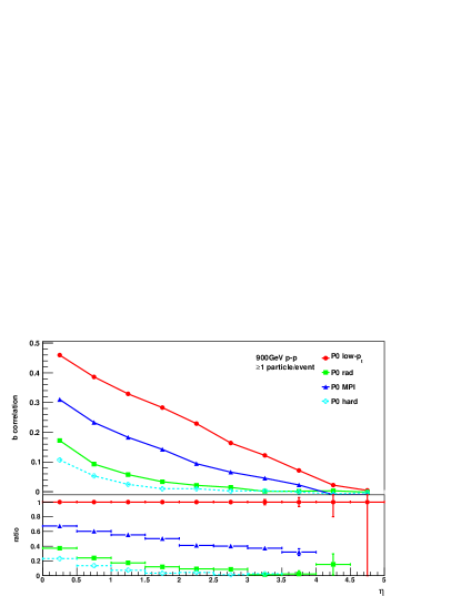
Figure 9: Inclusive $b$ correlation distribution for tune Perugia 0 particle production mechanisms: low-$p_{\perp}$, hard process (HARD), radiative production (RAD) and multi-parton interactions (MPI). Lower pane: ratio to the low-$p_{\perp}$ distribution.

As discussed above, however, one notes that the HARD component by itself only produces very short-range correlations, that drop off quickly to zero. Adding parton showers, in the RAD samples, extends the reach of these correlations somewhat further in $\eta$, including a small tail towards very large $\eta$, presumably generated by initial-state radiation from the beams.

Interestingly, the behaviour of the MPI component is somewhat different between the two kinds of models. In the old model, fig. 8, the MPI component becomes completely dominant at large $\eta$ and there has the same magnitude as the low-$p_{\perp}$ sample itself. In the new model, fig. 9, the MPI component alone drops off and is eclipsed by the shower component at the highest values of $\eta$, indicating a qualitative difference between the models, consistent with the new model deriving more of its total particle production from shower-related activity.

The effects of diffractive components, a non-zero contamination of which may be present especially in very inclusive minimum-bias measurements, are illustrated in fig. 10.

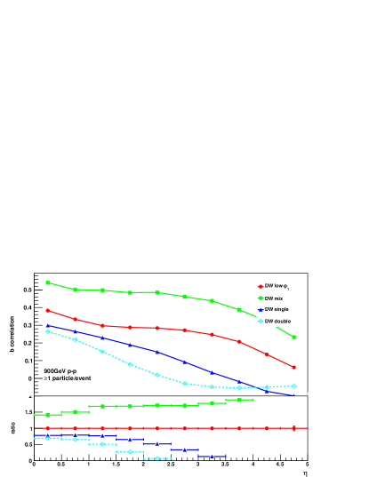
Figure 10: Inclusive $b$ correlation distribution for tune DW minimum bias sub-processes. Lower pane: ratio to the distribution of the low-$p_{\perp}$ sample.

The correlations in the SD and DD samples are intrinsically shorter-range than those of their non-diffractive counterparts, consistent with diffractive systems having a limited extension in rapidity.

However, we also see an interesting effect of combining the samples, namely that the correlations in the combined sample are stronger than in any of the individual components. It seems that, by mixing in less correlated diffractive components, we have actually enhanced the final correlations. What is going on? This effect can be illustrated by imagining we have two separate distributions, $A$ and $B$ (in our case represented, e.g., by the diffractive and non-diffractive samples). Imagine further that the fluctuations inside each sample are purely statistical, for illustration, such that the correlation strength inside each sample is zero. What will happen when we look at the combination $A+B$? If the mean of $A$ is smaller than that of $B$, then every event of type $A$ will look like it fluctuated down, systematically, from the mean of $A+B$, and conversely for the $B$ sample. In their combination, therefore, we will see a non-zero correlation if the mean values are different. Since the diffractive and non-diffractive event samples have very different average multiplicities (see table 3) this effect will lead to an increase in the correlations in the combined sample, as observed in fig. 10.

5.3 ‘Twisted’ b Correlations

We now turn to the dependence on azimuth of the forward-backward correlation strengths. A related type of correlations sensitive to both $\eta$ and azimuthal $\phi$ were recently highlighted by the CMS experiment Khachatryan:2010gv and have stimulated quite a lot of interest due to the observation of the so-called “ridge effect” in high-multiplicity events. The correlations presented in this report are somewhat simpler in spirit, and our focus is not primarily on high multiplicities, but we note that it could be an interesting follow-up study to determine whether twisted $b$-correlations could also be used to shed more light on the ridge.

We shall study the $\phi$ dependence of the $b$-correlations in two ways. The first is based only on the detector geometry. As this is independent of the event shape, no preference is given to any particular direction. The second method gives preference to the direction of the leading charged particle in the event. This will bias the zero point in $\phi$ to coincide with the most active part of the event.

In each case, we divide the $\phi$-plane into three regions of size $\Delta\phi=2/3\pi$. For the detector-defined geometry, we define a parallel, an opposite, and a transverse region. (Note: we use “parallel” and “opposite” here, to distinguish the geometry from Field’s “towards” and “away” regions, the latter of which we take to be defined relative to the direction of a lead particle or jet and not by the absolute detector geometry.) Quite arbitrarily, we define

• A parallel region covering the region $-\pi<\phi<-1/3\pi$ in absolute azimuth,

• An opposite region covering $0<\phi<2/3\pi$,

• A transverse region occupying the region between these, i.e., the slices $-1/3\pi<\phi<0$ and $2/3\pi<\phi<\pi$.

In calculating the correlation between $\eta-\phi$ regions the comparison is always to the parallel case on one side. We are aware that this is quite crude and that one could increase statistics by integrating over the location of the arbitrary azimuthal zero point, but point out that this is intended merely as a first exploration of the properties of ‘twisted’ correlations.

The terms of the $b$ correlation expression now refer to $\eta$-bins with a $\phi$-dependence. Hence, the correlation expression must include this new degree of freedom. Since all regions are a priori equivalent, the normalizing terms in $b$, $\left<n_{f}\right>^{2}$ and $\left<n_{f}^{2}\right>$, are taken simply from the parallel one. Only the product of activity in corresponding bins of $\eta-\phi$ are sensitive to the variation in $\phi$ region. The new expression, $b_{\phi}^{\mathrm{twist}}$, for the correlation becomes:

$$\centering b_{\phi}^{\mathrm{twist}}=\frac{\left<n_{b,\phi}n_{f,\parallel}\right>-\left<n_{f,\parallel}\right>^{2}}{\left<n_{f,\parallel}^{2}\right>-\left<n_{f,\parallel}\right>^{2}}.\@add@centering$$ (3)

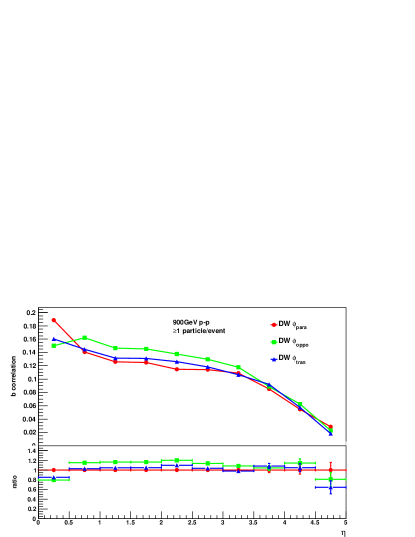
Figure 11: $b^{\mathrm{twist}}_{\phi}$ correlation distributions for hadron-level charged particles for DW Pythia tune for the three different combinations of $\phi$ regions, defined with respect to the absolute detector geometry. Lower pane: ratio to the parallel distribution.

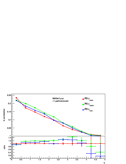
Figure 12: $b^{\mathrm{twist}}_{\phi}$ correlation distributions for hadron-level charged particles for the Perugia 0 tune for the three different combinations of $\phi$ regions, defined with respect to the absolute detector geometry. Lower pane: ratio to the parallel distribution.

Figures 11 and 12 show the three different types of correlations we can obtain for the detector-based geometry, for Pythia tunes DW and Perugia 0, respectively. As expected, both models exhibit a peak in the correlation at low $\eta$ in the parallel region, illustrating that the low-$\eta$ correlation is also most pronounced at low $\Delta\phi$. Beyond the first bin in $\eta$, however, the opposite correlation is strongest. This follows from momentum conservation, smeared out over $\eta$. The correlation with the transverse region is as close as we can come to defining an “underlying event” in an otherwise featureless minimum-bias event without a reference direction.

The difference in correlation strength between the three regions are not extremely large in absolute terms, however. This leads us to consider whether there is a way to enhance the differences while remaining in a minimum-bias context. By choosing the zero point of the $\phi$ coordinate, event by event, to be the direction of the leading (hardest) charged particle, we can now use the nomenclature of Field and define the towards region to include the azimuthal angles $\phi<\pm 1/3\pi$ around the lead particle, the away region covers $\pm 2/3\pi<\phi<\pm\pi$ and the transverse region lies in between, over $\pm 1/3\pi<\phi<\pm 2/3\pi$. We label the corresponding correlation $b^{\mathrm{lead}}_{\phi}$, to distinguish it from the detector-based one.

This orientation has a significant effect in particular for events with a semi-hard perturbative scattering, in which the main axis in the transverse plane becomes oriented to the production axis of the outgoing partons. The bias towards $\phi=0$ as the direction of the lead particle means that the three different $\phi$ regions can no longer be expected to have the same averages and variances. Nonetheless, in order to define a measure comparable to the one above, we shall still define the normalizing terms with respect to the towards region, so that eq. (3) still holds, although its statistical interpretation is modified.

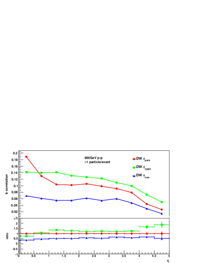
Figure 13: $b^{\mathrm{lead}}_{\phi}$ correlation distributions for hadron-level charged particles for the DW tune for the three different combinations of $\phi$ regions, defined with respect to the lead particle trajectory. Lower pane: ratio to the towards distribution.

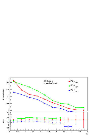
Figure 14: $b^{\mathrm{lead}}_{\phi}$ correlation distributions for hadron-level charged particles for the Perugia 0 tune for the three different combinations of $\phi$ regions, defined with respect to the lead particle trajectory. Lower pane: ratio to the towards distribution.

Redoing the twisted correlations with this definition of the zero point in azimuth, we obtain figures 13 and 14, for DW and Perugia 0, respectively, with the other tunes exhibiting similar qualitative features. The general remarks are similar to those for the detector-based geometry, but the differences between the regions are much more clearly visible. Also, the transverse region can here be clearly identified as lower than the others, consistent with its being an “underlying event” to the production of a “hard particle”.

6 Event Shapes

A further characteristic of the structure of the events in the minimum-bias sample can be gained by considering their eigenvalues along the principal event axes in the transverse plane. Obviously, we expect minimum-bias events to be much more uniform than, e.g., jet events, and hence to have smaller eigenvalues, but how much smaller? What is their average shape, and how much does it fluctuate between events?

To address these questions, and to gain a first idea of their sensitivity to the physics modeling, we consider the transverse thrust ($T_{t}$) and transverse minor ($M_{t}$) values and axes Banfi:2010xy .

6.1 Transverse Thrust

The transverse thrust axis can be found by maximizing the coincidence of an arbitrary vector with the dominant direction of particle flow in an event in $\phi$. The value of transverse thrust is then defined as:

$$\centering T_{\perp}=\max_{|\vec{n}_{\perp}|=1}\frac{\sum_{i}|\vec{n}_{\perp}\cdot\vec{p}^{i}_{\perp}|}{\sum_{i}|\vec{p}^{i}_{\perp}|}\leavevmode\nobreak\ ,\@add@centering$$ (4)

where $i$ runs over the charged tracks in the event, $\vec{n}_{\perp}$ is the transverse thrust axis unit vector and $\vec{p}^{i}_{\perp}$ is the track transverse momentum vector. The observable is bounded by $0.5<T_{\perp}<1.0$. Dijet-like events, where the highest-momentum particles are produced back to back, have a pencil-like shape in $\phi$, with particle production aligned predominantly along the axis. Such events have high transverse thrust values $\sim 1$. In contrast, in events where non-perturbative and/or MPI production is predominant, more particles will lie off the main production axis, giving a more circular distribution of tracks in $\phi$, for which the transverse thrust value will lie closer to $0.5$.

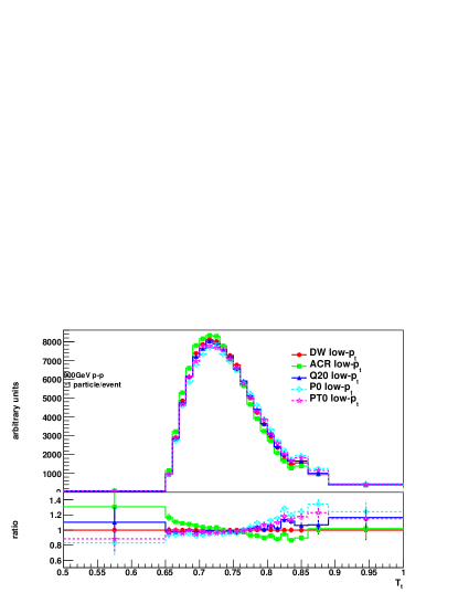
Figure 15: Transverse thrust distributions for the low-$p_{\perp}$ sub-sample of selected tunes, normalized to unit area. Lower pane: ratio to the DW distribution.

Fig.15 shows the transverse thrust distributions of the low-$p_{\perp}$ sub-samples of the selected tunes. Somewhat surprisingly, perhaps, the models agree to within 10–20% over most of the range. This presumably reflects the fundamental similarity between the MPI-based perturbative modeling in these tunes. A comparison with experimental data could give valuable insights on whether the real world is more or less “jetty” than these model predictions indicate.

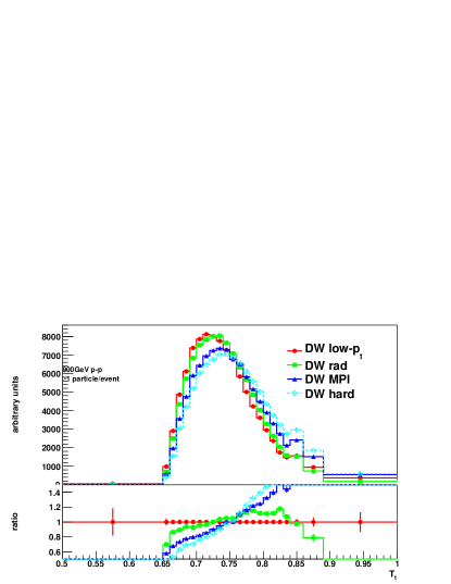
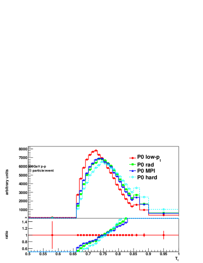
Figure 16: Transverse thrust distributions for the low-$p_{\perp}$ sample for a) DW and b) Perugia 0, normalized to unit area. Lower panes: ratio to the respective low-$p_{\perp}$ samples.

To further analyze the structure of this distribution, fig.16 shows the transverse thrust distributions for the HARD, RAD, and MPI samples, compared to the full low-$p_{\perp}$ simulation, for the DW (above) and Perugia 0 (below) tunes. For the HARD sample (i.e., before showering and MPI), the distributions are more pencil-like, peaking at somewhat higher values of $T_{\perp}$, illustrated by the dashed (cyan) curves. It is interesting that, in the old model (DW), the MPI component by itself (solid blue lines with triangular symbols) only reduces the peak value very slightly, whereas the addition of radiation (RAD: solid green lines with square symbols) produces a much larger shift. In the new model, however, the MPI and RAD samples each appear to give a similar-size shift. Despite their apparent similarities, there are therefore still interesting differences underlying these distributions, which, as we have argued, the measurement of $b$ correlations can help resolve.

6.2 Transverse Minor

The transverse minor axis lies perpendicular to the thrust axis in $\phi$. It is defined as:

$$\centering M_{\perp}=\max_{|\vec{n}_{\perp}|=1}\frac{\sum_{i}|\vec{n}_{\perp}\times\vec{p}^{i}_{\perp}|}{\sum_{i}|\vec{p}^{i}_{\perp}|}\leavevmode\nobreak\ ,\@add@centering$$ (5)

using the same definitions as in eq. (4).

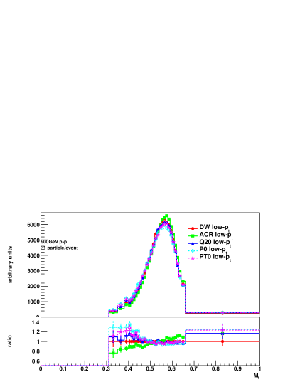
Figure 17: Transverse minor distributions for low-$p_{\perp}$ sub-samples of selected tunes, normalized to unit area. Lower pane: ratio to the DW distributions.

Fig.15 shows the transverse minor distributions of the low-$p_{\perp}$ sub-samples of the selected tunes. As before, the variations between models is relatively mild, with the contributions from each model component, fig. 18, exhibiting similar differences as for $T_{\perp}$.

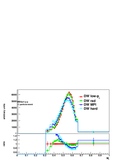
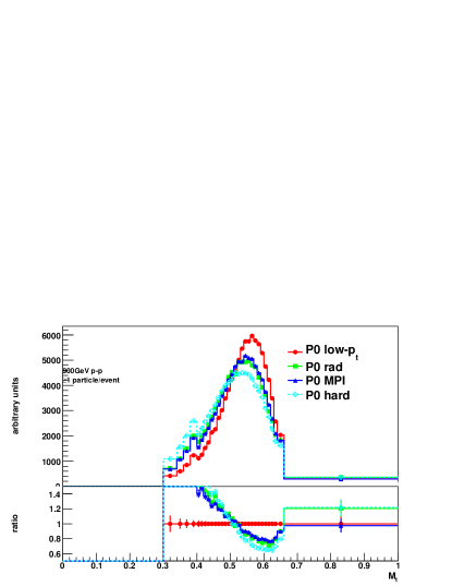
Figure 18: Transverse minor distributions for the low-$p_{\perp}$ sample for a) DW and b) Perugia 0, normalized to unit area. Lower panes: ratio to the respective low-$p_{\perp}$ samples.

7 Conclusion

We have illustrated that forward-backward correlations can be used to extract information on the relative strengths of different sources of particle production in minimum-bias events: models dominated by a single hard (dijet) interaction exhibit strong short-range correlations and weak long-range ones, while models with a larger component of soft production between the remnants generate stronger long-range correlations.

We propose to add these distributions to the “standard” ones already measured by the LHC experiments, and further to add correlations between different regions in azimuthal $\phi$, which we label ‘twisted’ forward-backward correlations.

We have illustrated these inferences by comparing a small set of recent tunes of the Pythia 6 Monte Carlo model. Although they are all based on a picture of multiple parton interactions (MPI) interfaced to the Lund string fragmentation model, they differ qualitatively in the shower and remnant modeling, and quantitatively in the fragmentation tuning and amount of showering vs. MPI.

We further believe that measurements of event shapes, such as transverse thrust and transverse minor, can help shed light on the overall properties and structure of minimum-bias events. For instance, a model with a strong dominance of perturbative (mini-)jet production should also predict event shapes closer to equivalent pQCD ones in dijet events, while models characterized by other particle production mechanisms should exhibit spectra further from the factorized pQCD prediction. In that context, however, the models studied here appear to give relatively similar results, presumably owing to the significant properties they share at the level of the underlying perturbative modeling.

Acknowledgments

The authors are grateful to S. Ferrag and to C. Buttar for their help and guidance. This research project has been supported by a Marie Curie Early Stage Research Training Studentship of the European Community’s Sixth Framework Programme under contract number (MRTN-CT-2006-035606-MCnet).

References

- (1) C. Buttar et al., (2008), 0803.0678.
- (2) ATLAS Collaboration, ATLAS Monte Carlo Tunes for MC09, ATL-PHYS-PUB-2010-002, 2010.
- (3) P. Z. Skands, Phys.Rev. D82, 074018 (2010), 1005.3457.
- (4) J. Butterworth et al., (2010), 1003.1643.
- (5) A. Abdesselam et al., (2010), 1012.5412.
- (6) M. Deak, F. Hautmann, H. Jung, and K. Kutak, (2010), 1012.6037.
- (7) ATLAS Collaboration, G. Aad et al., (2010), 1012.0791.
- (8) MCnet Collaboration, A. Buckley et al., (2011), 1101.2599.
- (9) CMS Collaboration, V. Khachatryan et al., JHEP 02, 041 (2010), 1002.0621.
- (10) ATLAS Collaboration, G. Aad et al., Phys. Lett. B688, 21 (2010), 1003.3124.
- (11) ALICE Collaboration, K. Aamodt et al., Eur.Phys.J. C68, 345 (2010), 1004.3514.
- (12) ALICE Collaboration, K. Aamodt et al., Eur.Phys.J. C68, 89 (2010), 1004.3034.
- (13) CMS Collaboration, V. Khachatryan et al., Phys. Rev. Lett. 105, 022002 (2010), 1005.3299.
- (14) ALICE Collaboration, K. Aamodt et al., Phys.Lett. B693, 53 (2010), 1007.0719.
- (15) CMS Collaboration, V. Khachatryan et al., (2010), 1011.5531.
- (16) ATLAS Collaboration, G. Aad et al., (2010), 1012.5104.
- (17) ATLAS Collaboration, G. Aad et al., ATL-COM-PHYS-2010-362 (2010).
- (18) T. Sjöstrand, S. Mrenna, and P. Z. Skands, JHEP 0605, 026 (2006), hep-ph/0603175.
- (19) B. Andersson, G. Gustafson, G. Ingelman, and T. Sjöstrand, Phys. Rept. 97, 31 (1983).
- (20) B. Andersson, Camb. Monogr. Part. Phys. Nucl. Phys. Cosmol. 7, 1 (1997).
- (21) T. Sjöstrand and M. van Zijl, Phys. Rev. D36, 2019 (1987).
- (22) T. Sjöstrand and P. Z. Skands, JHEP 0403, 053 (2004), hep-ph/0402078.
- (23) T. Sjöstrand and P. Z. Skands, Eur.Phys.J. C39, 129 (2005), hep-ph/0408302.
- (24) T. Sjöstrand and P. Z. Skands, Nucl.Phys. B659, 243 (2003), hep-ph/0212264.
- (25) TeV4LHC QCD Working Group, M. G. Albrow et al., (2006), hep-ph/0610012.
- (26) A. Buckley, H. Hoeth, H. Lacker, H. Schulz, and J. E. von Seggern, Eur.Phys.J. C65, 331 (2010), 0907.2973.
- (27) P. Z. Skands and D. Wicke, Eur.Phys.J. C52, 133 (2007), hep-ph/0703081.
- (28) T. Sjöstrand, S. Mrenna, and P. Skands, hep-ph/0603175 C66, 203 (March 2006).
- (29) UA5 Collaboration, Z. Phys. C, Particles and Fields 37, 191 (1988).
- (30) C. H. Christensen, J. J. Gaardhøje, K. Gulbrandsen, B. S. Nielsen, and C. Søgaard, Int.J.Mod.Phys. E16, 2432 (2007), 0712.1117.
- (31) CMS, V. Khachatryan et al., JHEP 09, 091 (2010), 1009.4122.
- (32) A. Banfi, G. P. Salam, and G. Zanderighi, JHEP 1006, 038 (2010), 1001.4082.