Transport in superlattices on single layer graphene.

Abstract

We study transport in undoped graphene in the presence of a superlattice potential both within a simple continuum model and using numerical tight-binding calculations. The continuum model demonstrates that the conductivity of the system is primarily impacted by the velocity anisotropy that the Dirac points of graphene develop due to the potential. For one-dimensional superlattice potentials, new Dirac points may be generated, and the resulting conductivities can be approximately described by the anisotropic conductivities associated with each Dirac point. Tight-binding calculations demonstrate that this simple model is quantitatively correct for a single Dirac point, and that it works qualitatively when there are multiple Dirac points. Remarkably, for a two dimensional potential which may be very strong but introduces no anisotropy in the Dirac point, the conductivity of the system remains essentially the same as when no external potential is present.

I Introduction

Graphene is one of the most interesting electronic systems to become available in the last few years Geim and Novoselov (2007); Castro-Neto et al. (2009). Graphene is a two-dimensional arrangement of carbon atoms in a triangular lattice with two atoms per unit cell. In graphene, the electronic low energy properties are governed by a massless Dirac Hamiltonian and the carriers moving in graphene have very interesting properties: the electronic spectrum is linear in the wavevector, and their states are chiral with respect the pseudospin defined by the two atoms of the crystal unit cell. These properties are responsible for exotic effects, such as a half-integer quantum Hall effect Novoselov et al. (2005); Zhang et al. (2005) and the Klein paradox – perfect transmission through potential barriers Kastnelson et al. (2006).

The application of electric fields via nano gate geometries makes it possible to subject the system to potentials varying on a short length scale. Using these techniques, recently it has been possible to study experimentally transport through $p$-$n$ junctions and $p$-$n$-$p$ junctions in graphene Huard et al. (2007); Young and Kim (2009); Stander et al. (2009); Jr et al. (2009); Russo et al. (2009). Theoretically, there has also been much effort devoted to the study of the spectra and the electronic transport through differently doped regions Pereira et al. (2006); Cheianov et al. (2007); Zhang and Fogler (2008); Beenakker (2008); Arovas et al. (2010) whose behavior differs from that of conventional two-dimensional electron gases.

A superlattice potential on top of graphene opens the possibility of tailoring its band structure and modifying its transport propertiesVázquez de Parga et al. (2008); Pletikosić et al. (2009); Tiwari and Stroud (2009); Guinea and Low (2010); Park et al. (2008a). In particular in the case of a one dimensional superlattice potential, the properties of the carriers are extremely sensitive to the amplitude $V_{0}$ and period $d$ of the superlattice. For a one dimensional superlattice, the velocity of the carriers is highly anisotropic Park et al. (2008b, c); Barbier et al. (2008) and the number of Dirac points at the Fermi energy can be altered by varying the product $V_{0}d$ Brey and Fertig (2009); Park et al. (2009); Barbier et al. (2010). Moreover, when the potential magnitude of the superlattice varies slowly in space, the electronic spectra develops a Landau level spectrum Sun et al. (2010). The effect of superlattice potentials due to external magnetic fields has also attracted a great deal of attention Dell’Anna and De Martino (2009); Snyman (2009); Tan et al. (2010); Dell’Anna and De Martino .

Several groups have numerically studied electronic transport perpendicular to the superlattice barriers Brey and Fertig (2009); Abedpour et al. (2009); Barbier et al. (2009, 2010); Wang and Zhu (2010); Yampol’skii et al. (2008); Bai and Zhang (2007). Starting from the theoretical universal value $\sigma_{0}=\frac{4}{\pi}\frac{e^{2}}{h}$Beenakker (2008), the conductivity increases with the product $V_{0}d$ and develops peaks at the critical values of $V_{0}d$ for which new Dirac points emergeBrey and Fertig (2009).

In this work we consider electronic transport in graphene in the presence of superlattice potentials that are piecewise constant. In the case of one-dimensional superlattices we study both transport parallel [Fig. 1(a)] and perpendicular [Fig. 1(b)] to the barriers. We also analyze transport in two-dimensional superlattices [Fig. 1(c)]. Analytical expressions for the conductivity are obtained by describing the carriers with the Dirac Hamiltonian and using the Kubo formula. These are compared with numerical results obtained using a tight-binding Hamiltonian for graphene in the presence of a superlattice potential and the Landauer-Büttiker formalism for obtaining the electrical conductivity in the presence of leads.

In the case of a one dimensional superlattice, we find that, as a function of the product $V_{0}d$, the conductivity parallel to the superlattice barriers, $\sigma_{\parallel}$, decreases quadratically from its value in the absence of the potential, $\sigma_{0}$, whereas in the perpendicular direction the conductivity $\sigma_{\perp}$ increases quadratically. The appearance of new Dirac points produces peaks in $\sigma_{\perp}$ and minima in $\sigma_{\parallel}$. For two-dimensional superlattices the conductivity depends on the relative values of the product $V_{0}d$ in different directions. Interestingly, for isotropic superlattice potentials, the conductivity is unaffected by the perturbation and remains at the universal value $\sigma_{0}$=$\frac{4}{\pi}\frac{e^{2}}{h}$. Further insight into the character of transport is obtained from the channel decomposition of the transmission matrix.

This paper is organized as follows. In Section II we present the analytical results for the conductivity obtained assuming independent anisotropic Dirac points. In Section III we present numerical results obtained with a microscopic tight-binding Hamiltonian and compare with the analytical expressions. Section IV is dedicated to the conclusions.

II One dimensional superlattice potential

II.0.1 Preliminaries.

The electronic structure of an infinitely large flat graphene flake is described by the Dirac Hamiltonian,

$$H_{0}=\hbar v_{F}\textbf{k}\cdot\mathbf{\sigma}\,\,\,$$ (1)

where $\hbar\textbf{k}$ is the momentum operator, $\mathbf{\sigma}$ are the Pauli matrices and $v_{F}\simeq 10^{6}m/s$ is the Fermi velocity. The two entries of the Dirac Hamiltonian correspond to the two carbon atoms in the unit cell in graphene.

The eigenvalues and eigenvectors of this Hamiltonian are $\varepsilon_{k,s}$=$sv_{F}\hbar k$ and $|s,\mathbf{k}>=\frac{e^{i\mathbf{k}\mathbf{r}}}{\sqrt{2}}\left(\begin{array}[]{c}1\\ se^{i\theta(\mathbf{k})}\end{array}\right)$, where $s=-1$ and $s=1$ describe the occupied and empty bands respectively. In the previous expressions $\theta(\mathbf{k})$ is the angle of the vector $\mathbf{k}$ with respect to the $\hat{k}_{x}$ direction.

II.0.2 Superlattice band structure.

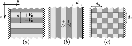
Figure 1: (Color online) Schematic representation of the superlattices used showing the axis selection. The system is infinite along the $x$-direction and has a finite length along the $y$-direction. The dashed patterns on each side of the $y$-direction indicate the leads for the Landauer conductance calculations. The superlattice barriers can be parallel (a) or perpendicular (b) to the direction of transport. We also consider a chessboard-like two dimensional superlattice potential in which $d_{y}\simeq d_{x}$ (c).

We consider a one-dimensional Kronig-Penney superlattice along the $\hat{x}$-direction (see Fig. 1(a)). The period of the potential is $d$, $V(x)=V(x+d)$ and $V(x)$=$V_{0}\,\textrm{sgn}(x)$ for $|x|<d/2$. For this potential it is possible to find an analytical expression for the band structure Barbier et al. (2010); Arovas et al. (2010), that in the limit of small wave vector and energies takes the form

$$\varepsilon(\mathbf{k})=\pm\hbar v_{F}\left(k_{x}^{2}+k_{y}^{2}\,\frac{\sin^{2}(\tilde{V})}{\tilde{V}^{2}}\right)^{1/2}\,\,\,,$$ (2)

where $\tilde{V}$=$\frac{V_{0}d}{2\hbar v_{F}}$. The group velocity of the state is anisotropically renormalized, and has a strong dependence on the direction of the wave vector $\mathbf{k}$Park et al. (2008b). At the Dirac point and for directions along the superlattice axis the velocity of the carriers is unaffected by the potentials, $v_{x}^{0}$=$v_{F}$. However the group velocity along the direction perpendicular to the superlattice direction is strongly renormalized and takes the form

$$v_{y}^{0}\simeq v_{F}\frac{|\sin(\tilde{V})|}{\tilde{V}}\,\,\,.$$ (3)

Whenever the superlattice parameters satisfy the condition,

$$\frac{V_{0}d}{\hbar v_{F}}=2\pi j\,\,\,\,\,j=1,2,3,...\,\,\,$$ (4)

the group velocity in the $\hat{y}$ direction vanishes and a new pair of Dirac points emerges from the original Dirac point, moving in opposite direction along the $\hat{k}_{y}$-directionBrey and Fertig (2009); Park et al. (2009). Near the new Dirac points and at low energy the dispersion is also linear and anisotropic. For the $j$-th pair of new Dirac points the velocity in the $\hat{x}$ and $\hat{y}$ directions have the expressionsBarbier et al. (2010),

$$v_{x}^{j} = \frac{j^{2}\pi^{2}}{\tilde{V}^{2}}v_{F}$$

$$v_{y}^{j} = v_{F}-v_{x}^{j}\,\,.$$ (5)

II.0.3 Electrical conductivity.

The conductivity in the collisionless limit has the expression Ziegler (2007); Ryu et al. (2007)

$$\sigma_{\mu\mu}(\omega)\!\!=\!\!-i\frac{e^{2}}{\hbar}g_{s}g_{v}\!\!\!\sum_{\mathbf{k},s,s^{\prime}}{\frac{f_{\mathbf{k},s^{\prime}}\!-\!f_{\mathbf{k},s}}{\varepsilon_{\mathbf{k},s^{\prime}}\!-\!\varepsilon_{\mathbf{k},s}}\,\,\frac{|<s,k|v_{\mu}|s^{\prime},k>|^{2}}{\varepsilon_{\mathbf{k},s^{\prime}}\!-\!\varepsilon_{\mathbf{k},s}\!-\!\hbar\omega\!-\!i\delta}}$$ (6)

where $s^{\prime}$ and $s$ are band indices, $f_{\mathbf{k},s}$ is the Fermi distribution function for the states $|s,\mathbf{k}>$, $v_{\mu}$ is the velocity operator in the $\hat{\mu}$ direction and $\delta$ is a positive infinitesimal constant. The conductivity contains a factor $g_{s}g_{v}$=4, which takes into account the spin and valley degeneracy. In the case of a single Dirac point with anisotropic velocities $v_{x}$ and $v_{y}$, expressed with a Dirac Hamiltonian of the form

$$H_{A}=\hbar(v_{x}k_{x}\sigma_{x}+v_{y}k_{y}\sigma_{y}),$$

one may show that the conductivity parallel and perpendicular to the potential barriers of the superlattice may be written in the form

$$\sigma_{\parallel}^{0}(\omega=0) = \frac{v_{y}^{0}}{v_{x}^{0}}\sigma_{0}=\sigma_{0}\frac{|\sin(\tilde{V})|}{\tilde{V}},$$

$$\sigma_{\perp}^{0}(\omega=0) = \frac{v_{x}^{0}}{v_{y}^{0}}\sigma_{0}=\sigma_{0}\frac{\tilde{V}}{|\sin(\tilde{V})|},$$ (7)

with $\sigma_{0}$ the conductivity of an isotropic Dirac Hamiltonian. The value of $\sigma_{0}$ depends on the order in which the zero frequency, zero temperature and vanishing “smearing parameter” $\delta$ Ryu et al. (2007) limits are takenLudwig et al. (1994); Ryu et al. (2007). However the form of the velocity rescaling of the conductivity is independent of the order in which the limits are taken.

In the case of several Dirac points in the spectrum, we assume that each of the points contributes to the conductivity in parallel and using Eq. (5), the conductivity takes the form,

$$\sigma_{\parallel} = \sigma_{0}\left(\frac{|\sin(\tilde{V})|}{\tilde{V}}+2\sum_{j=1}^{j_{max}}{\frac{\tilde{V}^{2}-(\pi j)^{2}}{(\pi j)^{2}}}\right)$$

$$\sigma_{\perp} = \sigma_{0}\left(\frac{\tilde{V}}{|\sin(\tilde{V})|}+2\sum_{j=1}^{j_{max}}{\frac{(\pi j)^{2}}{\tilde{V}^{2}-(\pi j)^{2}}}\right)$$ (8)

where $j_{max}$=$\mathrm{Integer}(\frac{\tilde{V}}{\pi})$ indicates the number of Dirac point pairs induced by the superlattice. From this expression we see that for small potentials the conductivity perpendicular to the superlattice barriers increases quadratically with $V_{0}d$, and each time a new pair of Dirac points emerges the conductivity exhibits a peak. In the direction parallel to the barriers, the conductivity decreases quadratically with $V_{0}d$ and dips when new Dirac points emerge.

We remark that in obtaining Eq. (8), we have assumed that each Dirac point contributes as an independent channel to the conductivity and that near each Dirac point the dispersion relation is linear over a wide range of the reciprocal space.

II.0.4 Mode dependent transmission.

The conductivity of a system governed by the Dirac equation with anisotropic velocities, $H=\hbar(v_{x}k_{x}\sigma_{x}+v_{y}k_{y}\sigma_{y})$, can be also obtained by calculating the transmission probability of modes confined in a stripe of width $W$ and length $L$ connected to heavily doped contactsTworzydlo et al. (2006); M. I. Katsnelson (2006); Das Sarma et al. (2010). For transport along the $\hat{x}$-direction, the transmission probability for a transverse mode has the form

$$T_{n}(\hat{x})=\frac{1}{\cosh^{2}(\frac{v_{y}}{v_{x}}q_{n}L)}\,,$$ (9)

where the transverse momentum $q_{n}$ depends on the details of the precise boundary condition of the strip Brey and Fertig (2006); Tworzydlo et al. (2006). For wide enough strips the conductivity of the system is independent of the boundary conditions and is found by summing over the modes,

$$\sigma_{xx} = g_{s}g_{v}\frac{L}{W}\frac{e^{2}}{h}\sum_{n}T_{n}(\hat{x})=\frac{e^{2}}{h}\frac{2L}{\pi}\int_{-\infty}^{\infty}\frac{dq}{\cosh^{2}(\frac{v_{y}}{v_{x}}qL)}$$ (10)

$$= \frac{4}{\pi}\frac{e^{2}}{h}\frac{v_{x}}{v_{y}}\,\,\,\,\mathrm{for}\,\,\,W>>L\,\,.$$

The conductivity in the $\hat{y}$ direction is obtained by interchanging $x$ and $y$ in the last equation. The condition for the existence of a well defined -size independent- conductivity is the dependence of the transmission probability on the product $qL$ (Eq. (9)) and the linear dispersion of the carriers. The condition $W\gg L$ allows the sum the transmissions over the modes to be written as an integral over $q$ in Eq. (10).

II.0.5 Two dimensional superlattice potential.

We consider a two dimensional superlattice potential on top a graphene sheet [as in Fig. 1(c)]. In second order perturbation theory the group velocity of quasiparticles with momentum $\mathbf{k}$ has the form Park et al. (2008b)

$$v_{\mathbf{k}}=v_{F}-v_{F}\sum_{\mathbf{G}\neq 0}\frac{2|U(\mathbf{G})|^{2}}{\hbar^{2}v_{F}^{2}|\mathbf{G}|^{2}}\sin^{2}\theta_{\mathbf{k},\mathbf{G}}\,\,\,,$$ (11)

where $\mathbf{G}$ and $U(\mathbf{G})$ are the reciprocal lattice vectors and the corresponding Fourier component of the external potential and $\theta_{\mathbf{k},\mathbf{G}}$ is the angle between $\mathbf{G}$ and $\mathbf{k}$. Using the same approximation as in the previous subsection the conductivity in the $\hat{x}$-direction takes the form

$$\sigma_{xx}=\sigma_{0}\frac{\hbar^{2}v_{F}^{2}-\sum_{\mathbf{G}\neq 0}2|U(\mathbf{G})|^{2}\frac{G_{y}^{2}}{|\mathbf{G}|^{4}}}{\hbar^{2}v_{F}^{2}-\sum_{\mathbf{G}\neq 0}2|U(\mathbf{G})|^{2}\frac{G_{x}^{2}}{|\mathbf{G}|^{4}}}\,\,\,\,.$$ (12)

The conductivity in the $\hat{y}$-direction is obtained by interchanging $G_{x}$ and $G_{y}$ in this expression. The striking result of Eq. (12) is that for symmetric superlattice potentials the conductivity in the $\hat{x}$ and $\hat{y}$ directions are equal and take the value of pristine graphene, $\sigma_{xx}$=$\sigma_{yy}$=$\sigma_{0}$=$\frac{4}{\pi}\frac{e^{2}}{h}$. The expression Eq. (11) has been obtained in second order perturbation theory and it is a good approximation provided that the superlattice potential does not induce new Dirac points. We expect that Eq. (12) will be valid in the same regime.

III Numerical calculations.

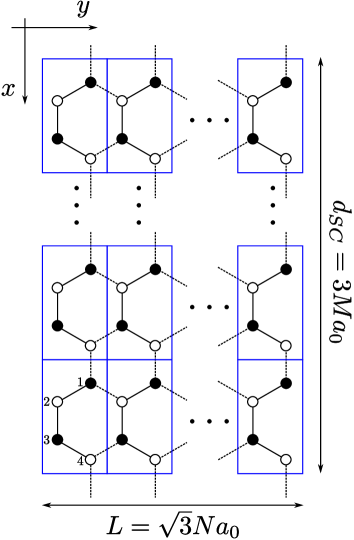
Figure 2: (Color online) Schematic representation of the superlattice used in the tight-binding calculations showing the axis selection. The system is infinite along the $x$-direction and has a finite length $L=\sqrt{3}Na_{0}$ along the $y$-direction. The superlattice has a vertical period $d=3Ma_{0}$ in which periodic boundary conditions are imposed.

In order to compute numerically the transport properties we describe the electronic states of a defect free graphene layer using the tight-binding approximation,

$$\hat{H}=-t_{g}\sum_{<ij>}\hat{c}^{\dagger}_{i}\hat{c}_{j}+\sum_{i}V_{i}\hat{c}^{\dagger}_{i}\hat{c}_{i}\,\,,$$ (13)

where $t_{g}=2\hbar v_{F}/3a_{0}$ denotes the hopping element between nearest carbon atoms on the hexagonal lattice, $a_{0}$ is the smallest carbon-carbon distance and $V_{i}$ is the potential applied to the lattice. The spin degree of freedom has been omitted due to degeneracy.

In order to analyze the different transport situations depicted in Fig. 1 we assume that the central region is a nanoribbon with armchair edges along the $\hat{x}$-direction as depicted in Fig. 2. The nanoribbon is constructed by repeating a unit cell composed of four atoms $N$ times along the $\hat{y}$-direction and $M$ times along the $\hat{x}$-direction. Thus, the length of the graphene stripe is $L=N\sqrt{3}a_{0}$. For describing the $W\gg L$ limit we impose periodic boundary conditions in the transversal direction $\hat{x}$ and define $q\in\left[-\pi/d_{SC},\pi/d_{SC}\right]$ as the corresponding wave vector, with $d_{SC}=3Ma_{0}$ being the vertical length of the supercell.

We connect the armchair edges of the nanoribbon to heavily doped graphene leads thus maintaining the graphene sublattice structure at the edgesSchomerus (2007); Blanter and Martin (2007); Brey and Fertig (2007); Burset et al. (2008, 2009). The corresponding self-energies on the graphene sites at the layer edges are approximated by a $4M\times 4M$ matrix with elements $\Gamma^{L,R}_{ij,\alpha\beta}=\delta_{ij}\gamma^{L,R}_{\alpha\beta}$, where $\alpha,\beta=1,\dots,4$ label the atomic sites within the unit cell and $i,j=1,\dots,M$ label the unit cells in the superlattice. Following the geometry depicted in Fig. 2, the elements of the self-energy matrix are explicitly defined as $\gamma^{L}_{22}=\gamma^{L}_{33}=\gamma^{R}_{11}=\gamma^{R}_{44}=i\sqrt{3}/2$ and $\gamma^{L}_{23}=\gamma^{L}_{32}=\gamma^{R}_{14}=\gamma^{R}_{41}=-1/2$Burset et al. (2008). Thus, we calculate the transmission at zero energy, $T(q)$, as

$$T(q)=4\mbox{Tr}\left[\hat{\Gamma}_{L}\hat{G}^{r}_{LR}(E=0,q)\hat{\Gamma}_{R}\hat{G}^{a}_{RL}(E=0,q)\right],$$ (14)

where $\hat{G}^{r,a}_{LR,RL}(E,q)$ are the $4M\times 4M$ retarded and advanced Green functions between the edges of the layer. Furthermore, for analyzing the transmission distribution it is useful to determine the eigenvalues $\tau_{\alpha}(q)$ of the transmission matrix $\hat{t}^{\dagger}\hat{t}$, where $\hat{t}=2\sqrt{\hat{\Gamma}_{L}}\hat{G}^{r}_{LR}(E,q)\sqrt{\hat{\Gamma}_{R}}$. From these eigenvalues one can determine the probability distribution $P(\tau)=\sum_{\alpha,q}\delta(\tau-\tau_{\alpha}(q))$ and the Fano factor

$$F=\frac{\sum\limits_{\alpha=1}^{4M}\sum\limits_{q}\tau_{\alpha}(q)\left(1-\tau_{\alpha}(q)\right)}{\sum\limits_{\alpha=1}^{4M}\sum\limits_{q}\tau_{\alpha}(q)}.$$ (15)

By integrating the transmission we compute the conductance of the system $G=(4e^{2}/\hbar)\int dq\mbox{Tr}\left[\hat{t}\hat{t}^{\dagger}\right]$, where both the spin and valley degeneracies have been taken into account. The resulting conductivity, within the limit $W\gg L$, is obtained by multiplying by the geometrical factor $L$.

III.1 Transport parallel to the superlattice barriers.

For studying the transport parallel to the superlattice, we consider a periodic one-dimensional potential along the $\hat{x}$-direction within the previous geometry as is schematically depicted in Fig. 1(a). The one-dimensional superlattice potential, $V_{i}$, has the piecewise constant form,

$$V_{i}=\left\{\begin{array}[]{ccl}V_{0}&,&0\leq x_{i}\leq\frac{d}{2}\\ -V_{0}&,&\frac{d}{2}<x_{i}\leq d\end{array}\right.,$$ (16)

where $d=d_{SC}=3Ma_{0}$ is the period of the potential.

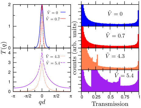
Figure 3: (Color online) In the left panels we plot, as function of $qd$, the transmission $T(q)$ per spin channel for a superlattice of period $d=42a_{0}$ and amplitudes $\tilde{V}=\frac{V_{0}d}{2\hbar v_{F}}=0$ and $\tilde{V}=0.7$ (top left panel) and for a period $d=54a_{0}$ and amplitudes $\tilde{V}=4.3$ and $\tilde{V}=5.4$ (bottom left panel). In the right panels we plot the distribution of the eigenvalues of the transmission matrix for the different values of $\tilde{V}$. The length of the stripe is $L=100\sqrt{3}a_{0}$.

In Fig. 3 we plot the transmission $T(q)$ as function of the product $qd$ for a superlattice of period $d=42a_{0}$ and amplitudes $V_{0}d=0$ and $V_{0}d=1.4\hbar v_{F}$ in the top left panel and for a period $d=54a_{0}$ and amplitudes $V_{0}d=8.6\hbar v_{F}$ and $V_{0}d=10.8\hbar v_{F}$ in the bottom left panel. The horizontal length of the graphene layer is $L=100\sqrt{3}a_{0}$. We also plot in the right panels of Fig. 3 the distribution of the eigenvalues of the transmission matrix.

In Fig. 4 we plot, as function of $V_{0}d$, the conductivity and the Fano factor obtained for a system of length $L$=$100\sqrt{3}a_{0}$ and for different values of the superlattice period, $d$.

We first discuss the case of potential barriers in the range $V_{0}<V_{c}=\frac{2\pi\hbar v_{F}}{d}$ [top panels of Fig. 3]. For these superlattices the original Dirac points are the only active transport channels. As a function of $q$ the transmission is peaked at $q$=0, and the width of the peak diminishes when $V_{0}d$ increases. The transmission fits very well to the functional form [see Eq. (9)] $T(q)=2/\cosh^{2}(\frac{\tilde{V}}{|\sin{\tilde{V}}|}qL)$, where the factor 2 accounts for the valley degeneracy and $\tilde{V}=\frac{V_{0}d}{2\hbar v_{F}}$. The corresponding distribution of the eigenvalues of the transmission matrix has the form $P(\tau)\sim 1/\tau\sqrt{1-\tau}$ indicating the pseudo-diffusive character of the transport in this range of potentials. The conductivity obtained by integrating the transmission is well-defined and, in this range of $V_{0}d$, has the form $\sigma_{\parallel}^{0}=\sigma_{0}\frac{|\sin(\tilde{V})|}{\tilde{V}}$ [see Fig. 4]. The Fano factor in this range of potentials is 1/3 in agreement with the pseudo-diffusive character of transport. We thus conclude that in the range of parameters $V_{0}d<{2\pi\hbar v_{F}}$ the transport is pseudo-diffusive, the conductivity only depends on the product $V_{0}d$ and has the form $\sigma_{\parallel}^{0}=\sigma_{0}\frac{|\sin(\tilde{V})|}{\tilde{V}}$.

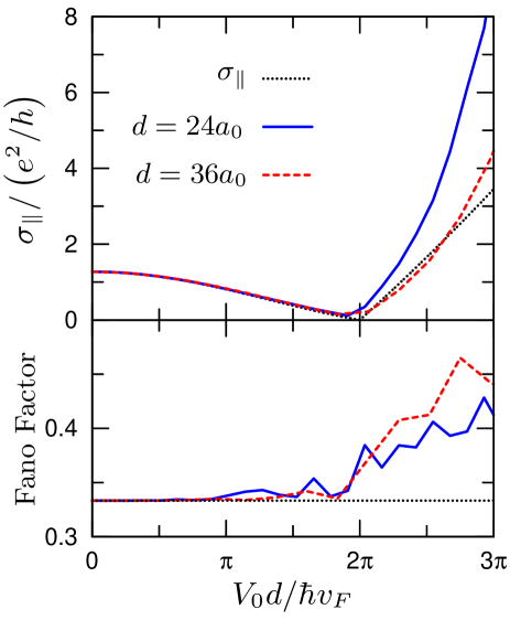
Figure 4: (Color online) Transport parallel to the superlattice barriers. Top (bottom) panel shows the conductivity (Fano factor) for a graphene sheet with $L=500\sqrt{3}a_{0}$ and superlattice period $d=24a_{0}$ (solid blue line) and $L=200\sqrt{3}a_{0}$ and superlattice period $d=36a_{0}$ (dashed red line) as a function of the normalized barrier height $V_{0}d$. Dotted line corresponds to the conductivity obtained in the continuum model assuming independent transport channels, Eq. (8), in the top panel and to the pseudo-diffusive value $F=1/3$ in the bottom panel.

For normalized barrier heights $V_{0}d$ larger than $2\pi\hbar v_{F}$ two new Dirac points per valley appearBrey and Fertig (2009); Park et al. (2009). These new Dirac points are new transmission channels in the system, that for transport parallel to the superlattice barriers are superimposed in reciprocal space upon the original Dirac points. The resultant transmission exhibits a wider distribution in reciprocal space [see bottom left panel of Fig. 3]. The width of the transmission can reach the edges of the reduced Brillouin zone $\pm\pi/d$ for small values of $L/d$. The corresponding distribution of the eigenvalues of the transmission matrix is a superposition of the distribution of each mode, and the corresponding Fano factor is different than $1/3$. The conductivity should be independent on the system size. We find that the value of $L$ where the conductivity is well defined depends on $d$ and coincides with the value of $L$ in which the transmission is non zero at the edges of the reduced Brillouin zone. In Fig. 4 we see that the general trend of the conductivity for values of $V_{0}d$ larger than $2\pi\hbar v_{F}$ is qualitatively described by the continuum model, Eq. (8). However the analytical model neglects some effects such as the coupling between the modes or the deviation from linear dispersion, so that in this range of superlattice parameters the conductivity depends separately on $V_{0}$ and $d$. The coupling between the modes also leads to a Fano factor with a value larger than $1/3$, and the transport is not pseudo-diffusive.

III.2 Transport perpendicular to the superlattice barriers.

In this section we consider a potential in the $\hat{y}$-direction and study the transport in the same direction, i.e. perpendicular to the superlattice barriers [see Fig. 1(b)]. Following the same geometry as in the previous section (see details in Fig. 2), we define a one-dimensional piecewise potential along the $\hat{y}$-direction as

$$V_{i}=\left\{\begin{array}[]{ccl}V_{0}&,&0\leq y_{i}\leq\frac{d}{2}\\ -V_{0}&,&\frac{d}{2}<y_{i}\leq d\end{array}\right.,$$ (17)

where $d=2n\sqrt{3}a_{0}$ is the period of the potential.

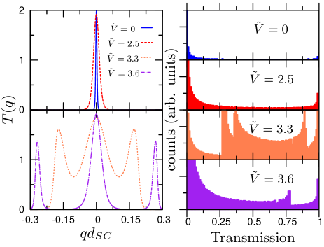
Figure 5: (Color online) In the left panels we plot, as function of $qd_{SC}$, the transmission $T(q)$ per spin channel for a superlattice of period $d=38.1a_{0}$ and normalized amplitudes $\tilde{V}=\frac{V_{0}d}{2\hbar v_{F}}=0$, $\tilde{V}=2.5$ (top left panel), $\tilde{V}=3.3$ and $\tilde{V}=3.6$ (bottom left panel). In the right panels we plot the distribution of the eigenvalues of the transmission matrix for the different values of $\tilde{V}$. The length of the stripe is $L=500\sqrt{3}a_{0}$.

In the left column of Fig. 5 we plot the transmission $T(q)$ as a function of $qd_{SC}$ for a superlattice with period $d=38.1a_{0}$ and amplitudes $V_{0}d=0$, $V_{0}d=5\hbar v_{F}$ (top left panel), $V_{0}d=6.6\hbar v_{F}$ and $V_{0}d=7.2\hbar v_{F}$ (bottom left panel). The horizontal length of the graphene strip is $L=500\sqrt{3}a_{0}$. In the right column of Fig. 5 we plot the corresponding distribution of the eigenvalues of the transmission matrix.

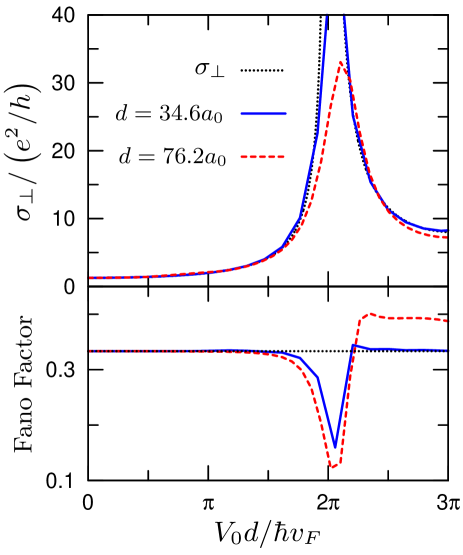
Figure 6: (Color online) Transport perpendicular to the superlattice barriers. Top (bottom) panel shows the conductivity (Fano factor) for a graphene sheet with $L=500\sqrt{3}a_{0}$ and superlattice periods $d=34.6a_{0}$ (solid blue line) $d=74.2a_{0}$ (dashed red line) as a function of the normalized barrier height $V_{0}d$. Dotted line corresponds to the conductivity obtained in the continuous model assuming independent transport channels, Eq. (8), in the top panel and to the pseudo-diffusive value $F=1/3$ in the bottom panel.

In the top panel of Fig. 6 we show, as function of $V_{0}d$, the conductivity for horizontal periods of $d=34.6a_{0}$ and $d=76.2a_{0}$, for a graphene sheet of length $L$=$500\sqrt{3}a_{0}$. In the bottom panel of Fig. 6 we plot the Fano factor for the same two values of the period of the superlattice.

In the range of potential barriers before the creation of new Dirac points, i.e. $V_{0}<V_{c}$, the behavior of the transmission is exactly the inverse of the previous case. The contribution to the transmission from each valley is superimposed as a sharp peak at $q=0$. However, contrary to the previous result, the width of the peak increases with the product $V_{0}d$. Following Eq. (9), the transmission is fitted to $T(q)=2/\cosh^{2}(\frac{|\sin{\tilde{V}}|}{\tilde{V}}qL)$. Subsequently, the distribution of the eigenvalues is that of pseudo-diffusive transport. On the other hand, when $V_{0}>2\pi\hbar v_{F}$, a pair of Dirac points is created for each valley. In the bottom panel of Fig. 5 we show how these new peaks split from the original ones until there are three almost independent contributions to the transmission. In this later case the distribution of eigenvalues for each mode returns to a form of the type $P(\tau)\sim 1/\tau\sqrt{1-\tau}$, indicative of pseudo-diffusive behavior. Before the new Dirac points are completely separated from the original ones, the coupling between modes produces a deviation from the pseudo-diffusive transport.

The behavior of the conductivity perpendicular to the barriers is completely different than the parallel case. The perpendicular conductivity presents peaks at the values of the normalized potential height where new Dirac points appear. The numerical calculated conductivity agrees very well with the analytical one, Eq. (8), even for values of $V_{0}d>2\pi\hbar v_{F}$. The Fano factor has the value $1/3$ for all values of $V_{0}d$ except near the values of $V_{0}d$ for which new Dirac appears. This indicates that, in this geometry, the Dirac points are weakly coupled and the approach of Section II for the conductivity is appropriate.

III.3 Transport in a two dimensional superlattice

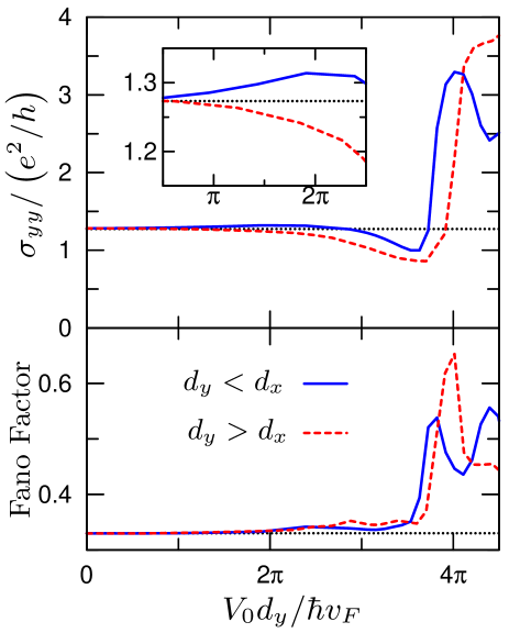
Figure 7: (Color online) In the top (bottom) panel we plot the conductivity (Fano factor) as a function of the normalized barrier height $V_{0}d_{y}$ for a graphene sheet in presence of a two dimensional superlattice with a fixed vertical period of $d_{x}=48a_{0}$ and different horizontal periods $d_{y}=45a_{0}$ (blue solid line) and $d_{y}=48.5a_{0}$ (red dashed line). The dotted line corresponds to the conductivity of pristine graphene ($\sigma_{0}$) in the top panel and to the pseudo-diffusive limit ($1/3$) in the bottom panel. The length of the graphene sheet is $L=200\sqrt{3}a_{0}$. Inset: the conductivity as a function of the normalized barrier height in the proximity of the critical potential $V_{c}$ in which a new pair of Dirac points is created.

One of the more striking results presented in Section II is that the conductivity of graphene in the presence of a symmetric two dimensional superlattice potential is $\frac{4}{\pi}\frac{e^{2}}{\hbar}$ independent of the period and the height of the potential barriers. In order to check this result we have built a chessboard-like potential combining piecewise potentials in the $\hat{x}$, Eq. (16), and $\hat{y}$, Eq. (17), directions in a way in which a potential barrier is always followed by a well along each direction (see Fig. 1(c)). The length of the period in the $\hat{x}$ and $\hat{y}$ directions is $d_{x}$ and $d_{y}$ respectively. Because the underlying triangular lattice of graphene, the period in both directions cannot be exactly equal.

The top panel of Fig. 7 shows the conductivity as a function of the potential height $V_{0}$ for a graphene layer with $L=200\sqrt{3}a_{0}$ and a fixed vertical period of $d_{x}=48a_{0}$. We plot the conductivity for two different horizontal periods $d_{y}=45a_{0}$ and $d_{y}=48.5a_{0}$. We compare these results with the isotropic conductivity of graphene $\sigma_{0}=\frac{4}{\pi}\frac{e^{2}}{h}$.

A remarkable result is that the conductivity in this potential remains almost constant in the range $V_{0}\gtrsim V_{c}$ where a new pair of Dirac points is created in the previously studied cases. Thus, in this range of potential barriers, Eq. (12) obtained in second order perturbation theory remains a good approximation according to the tight-binding results. Furthermore, the pseudo-diffusive behavior of transport is maintained for a large range of the potential barriers. In the bottom panel of Fig. 7 we show how the Fano factor is stable around the pseudo-diffusive value of $1/3$ while $V_{0}d_{y}\lesssim 4\pi\hbar v_{F}$. When $V_{0}d_{y}\sim 4\pi\hbar v_{F}$, which for the previous potentials corresponded to the creation of the second pair of Dirac points, the conductivity deviates from $\sigma_{0}$, the Fano factor increases and transport is no longer pseudo-diffusive. The approximation of weakly coupled Dirac points is then no longer applicable.

The small deviations from the conductivity of pristine graphene that occurs when $V_{0}d_{y}\sim 2\pi\hbar v_{F}$ can be more clearly appreciated in the inset of Fig. 7. Due to the geometry of the graphene layer, the period in both directions is never exactly the same. This affects the validity of Eq. (12) to a small degree. When $d_{y}\lesssim d_{x}$ the conductivity slightly increases from $\sigma_{0}$, presenting a positive slope, while if $d_{y}\gtrsim d_{x}$ the effect is the opposite. When the difference between both periods becomes larger the conductivity continuously evolves into the corresponding case of the previous sections (Figs. 4,6).

IV Conclusions

Superlattice potentials generically induce anisotropy in the dispersions near the Dirac points in graphene, and under certain circumstances may induce extra Dirac points at zero energy. In this work we demonstrated that when the Fermi energy passes through a spectrum with a single anisotropic Dirac point, the resulting conductivity can be expressed in a very simple way in terms of the velocities along the two principle directions of the anisotropy, and the conductivity for the corresponding isotropic Dirac point. The result can be generalized to the case of several Dirac points when they are sufficiently separated in momentum space so that a conductivity expressed as a sum over those of independent Dirac points is sensible. For a two-dimensional superlattice which induces little anisotropy in the spectrum, a remarkable result is that the conductivity is essentially unchanged from the result for pristine graphene, even if the velocity renormalization is quite large.

Numerical tight-binding calculations generally confirm this simple picture. In particular one finds the conductivity parallel and perpendicular to the superlattice barriers for a one-dimensional potential evolve in opposite directions with increasing $V_{0}d$, and that for a spectrum in which no new Dirac points have been generated there is quantitative agreement with the simple analytical model. As new Dirac points are introduced into the spectrum one finds dips in $\sigma_{\parallel}$ and peaks in $\sigma_{\perp}$ as expected, although the results are less quantitatively described by the continuum model, presumably because the wavefunctions cannot be uniquely associated with single Dirac points. Deviations of the Fano factor from pseudo-diffusive behavior confirm this interpretation.

These studies suggest that more complicated potentials could also yield behaviors in the conductance with simple interpretations. For example, a modulated superlattice potential yields a Landau level spectrum Sun et al. (2010), for which $\sigma_{\parallel}$ may have behavior reminiscent of edge state transport Iye . It is also interesting to speculate that for isotropic superlattice potentials, one may sufficiently slow the electron velocity so that electron-electron interaction effects become important Wang et al. (2010, 2011). We leave these questions for future research.

References

- Geim and Novoselov (2007) A. K. Geim and K. S. Novoselov, Nat.Mat. 6, 183 (2007).
- Castro-Neto et al. (2009) A. H. Castro-Neto, F. Guinea, N. M. R. Peres, K. S. Novoselov, and A. K. Geim, Rev. Mod. Phys. 81, 109 (2009).
- Novoselov et al. (2005) K. S. Novoselov, D. Jiang, T. Booth, V. V. Khotkevich, S. M. Morozov, and A. K. Geim, Nature 438, 197 (2005).
- Zhang et al. (2005) Y. Zhang, Y.-W. Tan, H. L. Stormer, and P. Kim, Nature 438, 201 (2005).
- Kastnelson et al. (2006) M. I. Kastnelson, K. S. Novoselov, and A.K.Geim, Nat.Phys. 2, 620 (2006).
- Huard et al. (2007) B. Huard, J. A. Sulpizio, N. Stander, K. Todd, B. Yang, and D. Goldhaber-Gordon, Phys. Rev. Lett. 98, 236803 (2007).
- Young and Kim (2009) A. F. Young and P. Kim, Nature Phys. 5, 222 (2009).
- Stander et al. (2009) N. Stander, B. Huard, and D. Goldhaber-Gordon, Phys. Rev. Lett. 102, 026807 (2009).
- Jr et al. (2009) J. V. Jr, G. Liu, W. Bao, and C. N. Lau, New Journal of Physics 11, 095008 (2009).
- Russo et al. (2009) S. Russo, M. F. Craciun, M. Yamamoto, S. Tarucha, and A. F. Morpurgo, New Journal of Physics 11, 095018 (2009).
- Pereira et al. (2006) J. M. Pereira, V. Mlinar, F. M. Peeters, and P. Vasilopoulos, Phys. Rev. B 74, 045424 (2006).
- Cheianov et al. (2007) V. V. Cheianov, V. Fal’ko, and B. L. Altshuler, Science 315, 1252 (2007).
- Zhang and Fogler (2008) L. M. Zhang and M. M. Fogler, Phys. Rev. Lett. 100, 116804 (2008).
- Beenakker (2008) C. W. J. Beenakker, Rev. Mod. Phys. 80, 1337 (2008).
- Arovas et al. (2010) D. P. Arovas, L. Brey, H. A. Fertig, E.-A. Kim, and K. Ziegler, New Journal of Physics 12, 123020 (2010).
- Vázquez de Parga et al. (2008) A. L. Vázquez de Parga, F. Calleja, B. Borca, M. C. G. Passeggi, J. J. Hinarejos, F. Guinea, and R. Miranda, Phys. Rev. Lett. 100, 056807 (2008).
- Pletikosić et al. (2009) I. Pletikosić, M. Kralj, P. Pervan, R. Brako, J. Coraux, A. T. NDiaye, C. Busse, and T. Michely, Phys. Rev. Lett. 102, 056808 (2009).
- Tiwari and Stroud (2009) R. P. Tiwari and D. Stroud, Phys. Rev. B 79, 205435 (2009).
- Guinea and Low (2010) F. Guinea and T. Low, Philosophical Transactions of the Royal Society A: Mathematical, Physical and Engineering Sciences 368, 5391 (2010).
- Park et al. (2008a) C.-H. Park, L. Yang, Y.-W. Son, M. L. Cohen, and S. G. Louie, Phys.Rev.Lett. 101, 126804 (2008a).
- Park et al. (2008b) C.-H. Park, L. Yang, Y.-W. Son, M. L. Cohen, and S. G. Louie, Nat.Phys. 4, 213 (2008b).
- Park et al. (2008c) C.-H. Park, Y.-W. Son, L. Yang, M. L. Cohen, and S. G. Louie, Nano Lett. 8, 2020 (2008c).
- Barbier et al. (2008) M. Barbier, F. M. Peeters, P. Vasilopoulos, and J. M. Pereira, Phys. Rev. B 77, 115446 (2008).
- Brey and Fertig (2009) L. Brey and H. A. Fertig, Phys. Rev. Lett. 103, 046809 (2009).
- Park et al. (2009) C.-H. Park, Y.-W. Son, L. Yang, M. L. Cohen, and S. G. Louie, Phys. Rev. Lett. 103, 046808 (2009).
- Barbier et al. (2010) M. Barbier, P. Vasilopoulos, and F. M. Peeters, Phys. Rev. B 81, 075438 (2010).
- Sun et al. (2010) J. Sun, H. A. Fertig, and L. Brey, Phys. Rev. Lett. 105, 156801 (2010).
- Dell’Anna and De Martino (2009) L. Dell’Anna and A. De Martino, Phys. Rev. B 79, 045420 (2009).
- Snyman (2009) I. Snyman, Phys. Rev. B 80, 054303 (2009).
- Tan et al. (2010) L. Z. Tan, C.-H. Park, and S. G. Louie, Phys. Rev. B 81, 195426 (2010).
- (31) L. Dell’Anna and A. De Martino, eprint arXiv:1101.1918v1.
- Abedpour et al. (2009) N. Abedpour, A. Esmailpour, R. Asgari, and M. R. R. Tabar, Phys. Rev. B 79, 165412 (2009).
- Barbier et al. (2009) M. Barbier, P. Vasilopoulos, and F. M. Peeters, Phys. Rev. B 80, 205415 (2009).
- Wang and Zhu (2010) L.-G. Wang and S.-Y. Zhu, Phys. Rev. B 81, 205444 (2010).
- Yampol’skii et al. (2008) V. A. Yampol’skii, S. Savel’ev, and F. Nori, New Journal of Physics 10, 053024 (2008).
- Bai and Zhang (2007) C. Bai and X. Zhang, Phys. Rev. B 76, 075430 (2007).
- Ziegler (2007) K. Ziegler, Phys. Rev. B 75, 233407 (2007).
- Ryu et al. (2007) S. Ryu, C. Mudry, A. Furusaki, and A.W.W. Ludwig, Phys. Rev. B 75, 205344 (2007).
- Ludwig et al. (1994) A. W. W. Ludwig, M. P. A. Fisher, R. Shankar, and G. Grinstein, Phys. Rev. B 50, 7526 (1994).
- Tworzydlo et al. (2006) J. Tworzydlo, B. Trauzettel, M. Titov, A. Rycerz, and C. W. J. Beenakker, Phys. Rev. Lett. 96, 246802 (2006).
- M. I. Katsnelson (2006) M. I. Katsnelson, Eur. Phys. J. B 51, 157 (2006).
- Das Sarma et al. (2010) S. Das Sarma, S. Adam, E. H. Hwang, and E. Rossi, eprint arXiv:1003.4731.
- Brey and Fertig (2006) L. Brey and H. A. Fertig, Phys. Rev. B 73, 235411 (2006).
- Schomerus (2007) H. Schomerus, Phys. Rev. B 76, 045433 (2007).
- Blanter and Martin (2007) Y. M. Blanter and I. Martin, Phys. Rev. B 76, 155433 (2007).
- Brey and Fertig (2007) L. Brey and H. A. Fertig, Phys. Rev. B 76, 205435 (2007).
- Burset et al. (2008) P. Burset, A. Levy Yeyati, and A. Martín-Rodero, Phys. Rev. B 77, 205425 (2008).
- Burset et al. (2009) P. Burset, W. Herrera, and A. Levy Yeyati, Phys. Rev. B 80, 041402 (2009).
- (49) A.P. Iyengar, Jianmin Sun, H.A. Fertig, and L. Brey, (unpublished).
- Wang et al. (2010) J. Wang, H. A. Fertig, and G. Murthy, Phys. Rev. Lett. 104, 186401 (2010).
- Wang et al. (2011) J. Wang, H. A. Fertig, G. Murthy, and L. Brey, Phys. Rev. B 83, 035404 (2011).