“Weak Quantum Chaos” and its resistor network modeling

Abstract

Weakly chaotic or weakly interacting systems have a wide regime where the common random matrix theory modeling does not apply. As an example we consider cold atoms in a nearly integrable optical billiard with displaceable wall (“piston”). The motion is completely chaotic but with small Lyapunov exponent. The Hamiltonian matrix does not look like one taken from a Gaussian ensemble, but rather it is very sparse and textured. This can be characterized by parameters $s$ and $g$ that reflect the percentage of large elements, and their connectivity, respectively. For $g$ we use a resistor network calculation that has a direct relation to the semi-linear response characteristics of the system, hence leading to a novel prediction regarding the EAR of cold atoms in optical billiards with vibrating walls.

I Introduction

So called ”quantum chaos” is the study of quantized chaotic systems. Assuming that the classical dynamics is fully chaotic, as in the case of a billiard with convex walls (Fig. ​​1), one expects the Hamiltonian to be like a random matrix with elements that have a Gaussian distribution. This is, of course, a sloppy statement, since any Hamiltonian is diagonal in some basis. The more precise statement behind random matrix theory (RMT) is following mario1 ; mario2 ; mario3 ; mario4 ; prosen1 ; prosen2 . Assume that there is a Hamiltonian $\mathcal{H}$ that generates chaotic dynamics, and consider an observable $F$ that has some classical correlation function $C(t)$, with some correlation time $t_{\mbox{\tiny R}}$. Then the matrix representation $F_{nm}$ in the basis of $\mathcal{H}$ looks like a random banded matrix. The bandwidth is $\hbar_{\mbox{\tiny Planck}}/t_{\mbox{\tiny R}}$. If $t_{\mbox{\tiny R}}$ is small, such that the bandwidth is large compared with the energy window of interest, then the matrix looks like taken from a Gaussian ensemble.

Our objective is to analyze the energy absorption rate (EAR) of billiards with vibrating walls, which is related to past studies of Nuclear friction wall1 ; wall2 ; wall3 . However, our interest is focused on 2D optical billiards nir1 ; nir2 ; nir3 ; nir4 ; kbw whose geometrical shape can be engineered. In this problem $\mathcal{H}$ is the Hamiltonian of the non-driven billiard, while $F_{nm}$ is the perturbation matrix due to the wall displacement. If the driving is not too strong we expect a linear relation

$$\dot{E}\ \ =\ \ G\ \dot{f}^{2}$$ (1)

where $\dot{f}$ is the RMS value of the vibrating wall velocity. If one further assumes that the billiard is strongly chaotic, then $G=G_{0}$ can be determined (Eq. ​​(98)) from simple kinetic considerations as in wall1 ; wall2 ; wall3 , leading to a variation of the so-called Wall-formula. Note that there is a strict analogy here with the Drude formula and the Joule law.

We consider completely chaotic billiards bunimovich ; young , with no mixed phase space, but we assume that they are only weakly chaotic bouncing1 ; bouncing2 ; triang ; spectral ; Backer ; wqc1 ; wqc2 ; cqb . This means that $t_{\mbox{\tiny R}}$ is much larger than the ballistic time $t_{\mbox{\tiny L}}$. Consequently, the EAR coefficient is

$$G\ \ =\ \ g\ G_{0}$$ (2)

with $g\neq 1$. In the classical analysis $g=g_{c}$ is related to classical correlations between the collisions with the vibrating walls. In the quantum analysis the first tendency is to assume $g\approx g_{c}$. In contrast to that we would like to highlight the possibility to observe $g\ll g_{c}$. This is the case if we have weak quantum chaos (WQC) circumstances, in which the traditional RMT modeling does not apply, meaning that $F_{nm}$ does not look like a typical random matrix. Rather, the distribution of its elements is log-wide (resembles a log-normal distribution), and it looks very sparse, as expected from Refs.sparse1 ; sparse2 ; sparse3 ; sparse4 . Consequently, the analysis of the EAR has to go beyond the familiar framework of linear response theory (LRT).

WQC circumstances are encountered in the analysis of any weakly chaotic or weakly interacting system. In the WQC regime the matrix $F_{nm}$ is formed of elements that have a log-wide distribution. The implied sparsity is important for the analysis of the EAR kbw ; cqb , as expected from semi-linear response theory (SLRT) kbr ; slr ; kbd . The main idea behind the theory is demonstrated in Fig. ​​2: one observes that the energy absorption process requires connected sequences of transitions between the energy levels of the system. Accordingly, the calculation of EAR requires a semi-linear resistor network calculation.

We can characterize the sparsity of the perturbation matrix by parameters ${s}$ and ${g_{s}}$ that reflect the percentage of large elements, and their connectivity, respectively. The parameter $g_{s}$ is defined through a resistor network calculation, and has a direct relation to the semi-linear response characteristics of the system, namely

$$g\ \ =\ \ g_{s}\ g_{c}$$ (3)

For a strictly uniform matrix ${g_{s}=s=1}$, for a Gaussian matrix ${s=1/3}$ and ${g_{s}\sim 1}$, while for sparse matrix ${s,g_{s}\ll 1}$. We would like to explore the dependence of $g_{c}$ and $g_{s}$ on the parameters $u$ and $h$ of the system. Disregarding the physical motivation, this exploration is mathematically interesting, because it introduces a “resistor network” perspective into RMT studies. Hence, it is complementary to the traditional spectral and intensity statistics investigations.

I.1 Generic parameters

For a billiard of linear size $L$ that has walls with radius of curvature $R$, as in Fig. ​​1, the Lyapunov time and the ballistic time are

$$t_{\mbox{\tiny R}}= R/v_{\mbox{\tiny E}}\ \ \ \ \$$ [Lyapunov time] (4)

$$t_{\mbox{\tiny L}}= L/v_{\mbox{\tiny E}}\ \ \ \ \$$ [Ballistic time] (5)

where ${v_{\mbox{\tiny E}}=(2E/\mathsf{m})^{1/2}}$ is the velocity of the particle. The quantization introduces an additional length scale into the problem, the de Broglie wavelength

$$\lambda_{\mbox{\tiny E}}\ \equiv\ \frac{2\pi}{k_{\mbox{\tiny E}}}\ \equiv\ \frac{h_{\mbox{\tiny Planck}}}{\mathsf{m}v_{\mbox{\tiny E}}}$$ (6)

Accordingly, the minimal model for the purpose of our study is featured by two small dimensionless parameters:

$$u= L/R =\mbox{[degree of deformation]}$$ (7)

$$\hbar= \lambda_{\mbox{\tiny E}}/L =\mbox{[scaled Planck]}\ =2\pi/(k_{\mbox{\tiny E}}L)$$ (8)

With the two classical time scales $t_{\mbox{\tiny L}}$ and $t_{\mbox{\tiny R}}$ one may associate two frequencies, while quantum mechanics adds an additional frequency that corresponds to the mean level spacing:

$$\Delta_{\mbox{\tiny L}}= 2\pi/t_{\mbox{\tiny L}}$$ (9)

$$\Delta_{\mbox{\tiny R}}= 2\pi/t_{\mbox{\tiny R}} =\ u\,\Delta_{\mbox{\tiny L}}$$ (10)

$$\Delta_{0}\equiv 2\pi/t_{\mbox{\tiny H}} =\ (\hbar/2\pi)^{d{-}1}\,\Delta_{\mbox{\tiny L}}$$ (11)

where $d{=}2$ is the dimensionality of the billiard. The WQC circumstances that we would like to consider are characterized by the following separation of scales:

$$\Delta_{0},\ \Delta_{\mbox{\tiny R}}\ \ll\ \Delta_{\mbox{\tiny L}}\ \ \ \ \ \ \ \ \ \mbox{[WQC]}$$ (12)

However, this is not a sufficient condition to observe WQC. The identification of the WQC regime in the ${(u,h)}$ space is an issue that we would have to address.

I.2 Detailed outline

The model.– In Sec. ​​(II) we define the model and explain the numerical procedure. Schematically the Hamiltonian of the system can be written as

$$\mathcal{H}_{\mbox{\tiny total}} = \mathcal{H}-f(t)F$$ (13)

$$= \mathcal{H}_{0}+U-f(t)F$$ (14)

where $\mathcal{H}_{0}$ describes the undeformed rectangular box, and $U$ describes the deformation of the fixed walls, and $F$ is the perturbation due to the displacement $f(t)$ of the moving wall (piston). The geometry of the billiard is characterized by $u$, while $\hbar$ defines via Eq. ​​(8) the energy window of interest.

Eigenstates.– Given $u$ and $\hbar$ we find the ordered eigenenergies $E_{n}$ of the Hamiltonian $\mathcal{H}$, within the energy window of interest. This is done using the boundary element method boundary . A representative eigenstate is presented in Fig. ​​3. If the deformation is small it is meaningful to represent it in the basis which is defined by $\mathcal{H}_{0}$. See for example Fig. ​​4. As the deformation becomes larger more and more levels are mixed as demonstrated in Fig. ​​5.

Perturbation matrix.– Once we have the eigenstates we calculate the matrix elements $F_{nm}$ of the perturbation term $F$, within the energy window of interest. An image of a representative matrix is shown in Fig. ​​6. The distribution of its elements is definitely not Gaussian, as shown in Fig. ​​7. In fact we see that the statistics of $|F_{nm}|^{2}$ resembles a log-normal distribution.

Bandprofile.– In order to characterize the bandprofile of the perturbation matrix we define in Sec. ​​(II) spectral functions $\bar{C}_{a}(r)$ and $\bar{C}_{s}(r)$ that are displayed in Fig. ​​8. We explain how $\bar{C}_{a}$ is semiclassically related to the power spectrum $\tilde{C}(\omega)$ of the collisions, and how $\bar{C}_{s}$ gives an indication for the sparsity of the matrix.

Sparsity.– We characterize the sparsity and the texture of the matrix by a parameter $g_{s}$ that is defined in Sec. ​​(III). The numerical results for $g_{s}$ are presented in Fig. ​​9. This characterization cares about the connectivity of the matrix elements, and is based on a calculation of a resistor network average. Some further details with respect to the resistor network average are given in App. ​​(A).

Classical analysis.– In Sec. ​​(IV) we provide a detailed analysis of the classical power spectrum $\tilde{C}(\omega)$. In particular, we derive an expression for the zero frequency peak, which reflects the long time correlations of the bouncing trajectories in our weakly chaotic billiard. App. ​​(B) provides optional perspectives with regard to this classical calculation.

Quantum analysis.– In Sec. ​​(V) we use 1st order perturbation theory for the analysis of the eigenstates of the deformed billiard, and hence get an approximation for $\tilde{C}(\omega)$. The validity of this approximation is very limited. We therefore fuse perturbation theory with semiclassical considerations in Sec. ​​(VI). This allows to obtain some practical approximations for $g_{c}$ and $g_{s}$.

The WQC regime.– Eventually we turn to define the borders of the WQC regime in the ${(u,h)}$ parameter space. This is also an opportunity to make a connection with previous works that concern spectral and intensity statistics for such type of weakly chaotic billiards.

Implications.– The relevance of the resistor network analysis to the EAR calculation is clarified in Sec. ​​(VIII), and the experimental feasibility of observing the implied SLRT anomaly is discussed in Sec. ​​(IX). A broader perspective with respect to EAR predictions is presented in Sec. ​​(X). In particular, we clarify how to bridge between what looks like contradicting results with regard to diffusive and diffractive systems, as opposed to ballistic billiards.

II The model, Numerics

The Hamiltonian of the system is

$$\mathcal{H}_{\mbox{\tiny total}}=\frac{\bm{p}^{2}}{2\mathsf{m}}+W_{\mbox{\tiny box}}\big{(}x,y\big{)}+W_{f}\big{(}x{-}f(t)D_{f}(y)\big{)}$$ (15)

We write it formally as in Eq. ​​(13), where $\mathcal{H}_{0}$ describes the undeformed rectangular box ${L_{x}\times L_{y}}$. The ballistic time is defined as $t_{\mbox{\tiny L}}=L_{x}/v_{\mbox{\tiny E}}$, which is the typical time for successive collisions with the piston. The term $U$ in the Hamiltonian is due to a deformation $D_{u}(y)$ of the left static wall. The amplitude of this deformation is $D_{0}\sim L_{y}^{2}/R$, while ${u\equiv L_{y}/R}$ is conveniently defined as the dimensionless deformation parameter. The driving term $-f(t)F$ is due to the deformation $f(t)D_{f}(y)$ of the right wall, leading to the identification

$$F\ \ =\ \ D_{f}(y)W_{f}^{\prime}(x)$$ (16)

For parallel displacement of a “piston” we set $D_{f}(y){=}1$. Note that $f(t)D_{f}$ unlike $D_{u}$ is assumed to be small compared with the de Broglie wavelength.

For a billiard system with “hard” walls the potential is zero inside the box, and become very large outside of the box. Accordingly, it is assumed that $W_{f}(r)=0$ for $r<0$, with a steep rise as $r$ becomes $>0$. Accordingly, the penetration distance upon collision is much smaller compared with the linear dimension $L$ of the box. Say that the force which is exerted on the particle by the piston is $W_{f}^{\prime}(r)=F_{0}$ for $r>0$ and zero otherwise, then it is assumed that $E/F_{0}\ll L$, where $E$ is the kinetic energy of the particle inside the box. Below we take the limit $F_{0}\rightarrow\infty$.

Following frc ; dil ; wlf we discuss the definition and the calculation of the spectral function $\tilde{C}(\omega)$ that describes the fluctuations of $F$ in the non-driven billiard system. We first discuss the classical and then turn to the quantum.

Classical.– In the classical context the Hamiltonian $\mathcal{H}$ can be used to generate a trajectory ${(t_{j},y_{j},\theta_{j})}$, where $j$ labels successive collisions with the piston at ${(0,y_{j})}$ with incident angle $\theta_{j}$. Consequently, the associated $F(t)$ consists of impulses of height $F_{0}$ whose duration is $2\mathsf{m}v_{\mbox{\tiny E}}\cos(\theta_{j})/F_{0}$. In the hard wall limit one can write formally

$$F(t)\ \ =\ \ \sum_{j}2\mathsf{m}v_{\mbox{\tiny E}}\ \cos(\theta_{j})\ D_{f}(y_{j})\ \delta(t-t_{j})$$ (17)

Assuming ergodic motion, the auto-correlation function of $F(t)$ can be calculated from the time dependence of a single trajectory that has some long duration $t_{\infty}$

$$C(t)=\langle F(t)F(0)\rangle=\overline{F(t)F(0)}$$ (18)

The associated power spectrum is:

$$\tilde{C}_{\mbox{\tiny cl}}(\omega) \equiv \int_{-\infty}^{\infty}C(t)\,\mbox{e}^{i\omega t}dt=\frac{1}{t_{\infty}}|\tilde{F}(\omega)|^{2}$$ (19)

$$= \frac{1}{t_{\infty}}\left|\sum_{j}2mv_{\mbox{\tiny E}}\cos(\theta_{j})D_{f}(y_{j})\mbox{e}^{i\omega t_{j}}\right|^{2}$$ (20)

If we regard the impulses as uncorrelated we get the result

$$\tilde{C}_{\mbox{\tiny cl}}(\omega)\ \ \rightarrow\ \ \left[\frac{8}{3\pi}\frac{\mathsf{m}^{2}v_{\mbox{\tiny E}}^{3}}{L_{x}}\right]\ \ \equiv\ \ C_{\infty}$$ (21)

which holds in the $\omega\rightarrow\infty$ limit. More details about this calculation and its refinement will be presented in Sec. ​​(IV).

Quantum.– The unperturbed energy levels of the rectangular box are

$$E_{\bar{\bm{n}}}\ =\ E_{n_{x}n_{y}}\ =\ \frac{1}{2\mathsf{m}}\left[\left(\frac{\pi n_{x}}{L_{x}}\right)^{2}+\left(\frac{\pi n_{y}}{L_{y}}\right)^{2}\right]$$ (22)

with the mean level spacing

$$\Delta_{0}\ \ =\ \ \frac{2\pi}{\mathsf{m}L_{x}L_{y}}$$ (23)

For a given deformation we diagonalize $\mathcal{H}$, and find the ordered eigenenergies $E_{n}$ with ${n=1,2,3,...}$, within an energy window of interest which is characterized by the dimensionless parameter $\hbar$. This is done using the boundary element method boundary . Each eigenstates $\psi(x,y)$ is represented by a boundary function $\varphi(y)\equiv\psi^{\prime}(0,y)$, where the normal derivative is with respect to $x$ at the position ${x{=}0}$ of the piston. Consequently, the matrix elements of $F$ are

$$F_{nm}=-\frac{1}{2\mathsf{m}}\int_{0}^{L_{y}}\varphi^{(n)}(y)\varphi^{(m)}(y)\ D_{f}(y)dy$$ (24)

Given $F_{nm}$ one can calculate the quantum mechanical version of the spectral function

$$\tilde{C}_{\mbox{\tiny qm}}(\omega)=\sum_{m}|F_{nm}|^{2}\ 2\pi\delta(\omega-(E_{m}{-}E_{n}))$$ (25)

where it is implicit that the delta functions have a finite smearing width related to the measurement time $t_{\infty}$, and an average over the reference state (${E_{n}\sim E}$) is required to reflect the associated uncertainty in energy.

Correspondence.– For a chaotic system, if the correlation time is short, one expects quantum-to-classical correspondence (QCC) with regard to $\tilde{C}(\omega)$. It follows from Eq. ​​(25) that this spectral function should reflect the bandprofile of the perturbation matrix mario1 ; mario2 ; mario3 ; mario4 . Let us express this observation in a convenient way that allows a practical procedure for numerical verification. We calculate $F_{nm}$ in an energy window of interest, and define the associated matrix

$$\bm{X}\ \ =\ \ \{|F_{nm}|^{2}\}$$ (26)

The bandprofile $\bar{C}_{a}(r)$ is defined by the average of the elements $X_{nm}$ along the diagonals $n{-}m=r$. In the same way we also define a median based bandprofile $\bar{C}_{s}(r)$. Given that the mean level spacing $\Delta_{0}$ is small compared with the energy range of interest, the correspondence between $\tilde{C}_{\mbox{\tiny qm}}(\omega)$ and $\tilde{C}_{\mbox{\tiny cl}}(\omega)$ can be expressed as:

$$\bar{C}_{a}(n-m)\ \ \approx\ \ \left(\frac{2\pi}{\Delta_{0}}\right)^{-1}\ \tilde{C}_{\mbox{\tiny cl}}(E_{n}-E_{m})$$ (27)

In particular, it follows from Eq. ​​(21) that the unrestricted average value of the elements $X_{nm}$ is

$$\langle\langle\bm{X}\rangle\rangle_{\infty}\ \ =\ \ \left(\frac{8}{3\pi}\right)\frac{\mathsf{m}v_{\mbox{\tiny E}}^{3}}{L_{y}L_{x}^{2}}$$ (28)

In fact this result can be established without relaying on QCC considerations via a sum rule that we discuss in Sec. ​​(VI), and the same result is also obtained from the zero order evaluation of matrix as described in Sec. ​​(V). Whenever applicable we re-scale the numerical results with respect to this reference value.

The applicability of the QCC relation Eq. ​​(27), to the analysis of our billiard system is confirmed in Fig. ​​8, down to very small frequencies. We also see that

$$\bar{C}_{s}(r)\ \ \ll\ \ \bar{C}_{a}(r)\ \ \rightarrow\ \ \langle\langle\bm{X}\rangle\rangle_{\infty}$$ (29)

where the value on the right is obtained in the limit ${r\rightarrow\infty}$. The inequality $\bar{C}_{s}\ll\bar{C}_{a}$ means that the value of the typical matrix element is very small compared with the average value. We are therefore motivated to define notions of sparsity and texture in Sec. ​​(III).

III Sparsity and texture

For strongly chaotic systems the elements within the band have approximately a Gaussian distribution. But for WQC the matrix becomes sparse and textured as demonstrated in Fig. ​​6. These features go beyond the semiclassical analysis of the bandprofile. The sparsity is related to the size distribution of the in-band elements: Loosely speaking one may say that only a small fraction ($s$) of elements are large, while most of the elements are very small (for a precise definition of $s$ see below). The texture refers to the non-random arrangement of the minority of large elements.

In the WQC regime the size distribution of the in-band elements becomes log-wide (approximately log-normal) as seen in Fig. ​​7. This is reflected by having ${\bar{C}_{s}(r)\ll\bar{C}_{a}(r)}$ as seen in Fig. ​​8. Accordingly, an optional measure for sparsity is the parameter $q$ which is defined as the ratio of the median to the average.

The sparsity and the texture of $F_{nm}$ are important for the analysis of the energy absorption rate as implied by SLRT. Accordingly, it is physically motivated to characterize the sparsity by a resistor network measure $g_{s}$ that reflects the connectivity of the elements, and hence has a direct relation to the semi-linear response characteristics of the system. The precise definitions of $g_{s}$ is given below. For a strictly uniform matrix ${g_{s}=s=1}$, for a Gaussian matrix ${s=1/3}$ and ${g_{s}\sim 1}$, while for sparse matrix ${s,g_{s}\ll 1}$. The dependence of the sparsity on the energy and on the degree of deformation is demonstrated in Fig. ​​9, and is related to the mixing of the levels in Fig. ​​5.

Definition of $s$.– Define a matrix $\bm{X}$ whose elements are ${X_{nm}=|F_{nm}|^{2}}$. Associate with it an untextured matrix $\bm{X}^{\mbox{\tiny utx}}$ and a uniformized matrix $\bm{X}^{\mbox{\tiny unf}}$ that have the same bandprofile $C(r)$. The former is obtained by performing random permutations of the elements along the diagonals, while the latter is obtained by replacing each of the elements of a given diagonal by their average. The participation number (PN) of a set $\{X_{i}\}$ is defined as ${\left(\sum_{i}X_{i}\right)^{2}/\sum_{i}X_{i}^{2}}$, and reflects the number of the large elements. Here the index is ${i=(n,m)}$. The PN of $\{X_{nm}\}$ counts the number of large elements in the matrix. The PN of $\{X_{nm}^{\mbox{\tiny unf}}\}$ counts the number of the in-band elements. Accordingly, the ratio constitutes a measure for sparsity:

$$s\ \ =\ \ s[\bm{X}]\ \ \equiv\ \ \frac{\mbox{PN}\left[\bm{X}\right]}{\mbox{PN}\left[\bm{X}^{\mbox{\tiny unf}}\right]}$$ (30)

It should be clear that $\bm{X}$ and $\bm{X}^{\mbox{\tiny utx}}$ have the same $s$ but only the former might have texture. So the next question is how to define texture avoiding a subjective visual inspection.

Definition of $g_{s}$.– Complementary information about the sparsity of the matrix, that takes into account the texture as well, is provided by the resistor network measure $g_{s}$. Coming back to $X_{nm}$ we can associate with it a matrix

$$G_{nm}=2F(n{-}m)\,\frac{X_{nm}}{(n-m)^{2}}$$ (31)

where $\sum_{r}F(r)=1$ is a weight function whose width should be quantum mechanically large (i.e. $\gg 1$) but semiclassically small (i.e. $\lesssim$ the bandwidth). With such choice the $G_{nm}$ are proportional to the Fermi-golden rule transition rates that would be induced by a low-frequency driving $-f(t)F$. Optionally we can regard these $G_{nm}$ as representing connectors in a resistor network, as in Fig. ​​2. The inverse resistivity of the strip can be calculated using standard procedure, as in electrical engineering, and the result we call $\langle\langle\bm{X}\rangle\rangle_{s}$. For more details see App. ​​(A). It is useful to notice that if all the elements of $\bm{X}$ are identical then $\langle\langle\bm{X}\rangle\rangle_{s}$ equals the same number. More generally $\langle\langle\bm{X}\rangle\rangle_{s}$ is smaller than the conventional algebraic average $\langle\langle\bm{X}\rangle\rangle_{a}$ (calculated with the same weight function). Accordingly, the resistor network quantity $\langle\langle\bm{X}\rangle\rangle_{s}$ can be regarded as a smart average over the elements of $\bm{X}$, that takes their connectivity into account. Consequently, it is natural to define a physically motivated resistor-network measure for sparsity and texture:

$$g_{s}\ \ =\ \ g_{s}[\bm{X}]\ \ \equiv\ \ \frac{\langle\langle\bm{X}\rangle\rangle_{s}}{\langle\langle\bm{X}\rangle\rangle_{a}}$$ (32)

One can show that $\langle\langle\bm{X}\rangle\rangle_{s}$ is strictly bounded from below by the harmonic average. In practice the geometric average or the median provide better lower bounds. In the RMT context a realistic estimate for $\langle\langle\bm{X}\rangle\rangle_{s}$ can be obtained using a generalized variable-range-hopping procedure (see kbd for details).

Additional definitions.– If the elements $X_{nm}$ have a well defined average $\langle\langle\bm{X}\rangle\rangle_{\infty}$ in the limit of infinite truncation, then it is convenient to define

$$g_{c}\ \ \equiv \ \ \frac{\langle\langle\bm{X}\rangle\rangle_{a}}{\langle\langle\bm{X}\rangle\rangle_{\infty}}$$ (33)

$$g\ \ \equiv \ \ \frac{\langle\langle\bm{X}\rangle\rangle_{s}}{\langle\langle\bm{X}\rangle\rangle_{\infty}}\ \ =\ \ g_{s}\ g_{c}$$ (34)

Later, in Sec. ​​(VIII), we discuss the physical significance of $g$, and identify it as the dimensionless absorption coefficient. In particular, $g_{c}$ is identified as the dimensionless absorption coefficient in the classical calculation, which is determined by taking into account classical correlations. In the quantum case we have an additional suppression factor $g_{s}$ due to the sparsity of the perturbation matrix.

IV Classical analysis of $\tilde{C}(\omega)$

Let us assume that we have a collision in angle $\theta$ with the flat piston. The force which is exerted on the particle during the collision is $F_{0}$, such that the impact is

$$q_{\theta}=2\mathsf{m}v_{\mbox{\tiny E}}\cos(\theta)$$ (35)

Consequently, the force $F(t)$ looks like a train of spikes as in Eq. ​​(17). Note that the duration of a collision is $q_{\theta}/F_{0}$. In the absence of deformation the time distance between the spikes is

$$\tau_{\theta}=\frac{2L_{x}}{v_{\mbox{\tiny E}}\cos\theta}$$ (36)

where $\theta$ is constant of the motion. For the following calculations it is useful to define the following averages:

$$C_{\infty}=\left\langle\left(\frac{q_{\theta}^{2}}{\tau_{\theta}}\right)\right\rangle_{\theta} = \frac{8}{3\pi}\frac{\mathsf{m}^{2}v_{\mbox{\tiny E}}^{3}}{L_{x}}$$ (37)

$$c_{0}=\left\langle\left(\frac{q_{\theta}}{\tau_{\theta}}\right)^{2}\right\rangle_{\theta} = \frac{3}{8}\frac{\mathsf{m}^{2}v_{\mbox{\tiny E}}^{4}}{L_{x}^{2}}$$ (38)

$$c_{\infty}=\left\langle\left(\frac{q_{\theta}}{\tau_{\theta}}\right)\right\rangle_{\theta}^{2} = \frac{1}{4}\frac{\mathsf{m}^{2}v_{\mbox{\tiny E}}^{4}}{L_{x}^{2}}$$ (39)

$$\mbox{Var}\!\left[\frac{q}{\tau}\right]\equiv c_{0}-c_{\infty} = \frac{1}{8}\frac{\mathsf{m}^{2}v_{\mbox{\tiny E}}^{4}}{L_{x}^{2}}$$ (40)

If we have a very small $u$ the effect would be to ergodize $\theta$ with some rate $\gamma_{\theta}$. After time $t$ the number ($\#$) of collisions is ${t/\tau_{\theta}}$ and consequently the deviation of the perturbed trajectory is multiplied by $(1+L/R)^{\#}\approx\exp\left((v_{\mbox{\tiny E}}t/R)\cos(\theta)\right)$. Accordingly, the instability exponent is

$$\gamma_{\theta}\ \approx\ \gamma_{0}+\frac{v_{\mbox{\tiny E}}}{R}\cos(\theta)$$ (41)

For sake of generality we have added a background term $\gamma_{0}$. This background term would arise if the upper or lower walls were deformed, or if the potential floor were not flat. A non zero $\gamma_{0}$ is unavoidable in a realistic system. As we shall see shortly the effect of the deformation is twofold. The primary effect is to ergodize $\theta$, and the secondary effect is to modify the small $\omega$ spectral content of the fluctuations.

Power spectrum.– Let us define $F_{\theta}(t)$ as the temporal “signal” which is associated with a trajectory that starts at the piston with $\theta$ collision angle. This signal consists of delta spikes, the first one being $q_{\theta}\delta(t)$. The correlation function can be expressed as

$$\langle F(0)F(t)\rangle=\left\langle\frac{q_{\theta}}{\tau_{\theta}}F_{\theta}(t)\right\rangle_{\theta}\ \ \ \ \ \ \ \ \ \$$ (42)

$$=\left\langle\frac{q_{\theta}^{2}}{\tau_{\theta}}\right\rangle_{\theta}\delta(t)\ +\ \mbox{correlations}$$ (43)

where the first term represents the self-correlation of the spikes. It is convenient to subtract from $\langle F(0)F(t)\rangle$ its global offset, and to define the correlation function as

$$C(t)\ \ =\ \ \langle F(0)F(t)\rangle-\langle F\rangle^{2}$$ (44)

The associated power spectrum is the Fourier transform:

$$\tilde{C}(\omega)=\left\langle\frac{q_{\theta}}{\tau_{\theta}}\tilde{F}_{\theta}(\omega)\right\rangle_{\theta}-\left\langle\frac{q_{\theta}}{\tau_{\theta}}\right\rangle_{\theta}^{2}2\pi\delta(\omega)$$ (45)

Note that $\tilde{F}_{\theta}(\omega)$ is the FT of $F_{\theta}(t)$. It is not the same as $\tilde{F}(\omega)$ of Eq. ​​(19). The latter has a random phase due to a time displacement of the time origin, while in the case of $F_{\theta}(t)$ the time origin is fixed by the presence of $F(0)$ in Eq. ​​(42).

Infinite frequency limit.– The first obvious observation is that that for large frequencies the power spectrum becomes flat and reaches a constant value that reflects the self-correlation peak of Eq. ​​(43)

$$\tilde{C}(\infty)\ \ =\ \ \left\langle\frac{q^{2}}{\tau}\right\rangle\ \ =\ \ C_{\infty}$$ (46)

where $C_{\infty}$ is given by Eq. ​​(37). This result, if it is a applied to finite frequencies, is termed in the literature “the white noise approximation”.

Zero deformation.– Let us consider the non-deformed integrable billiard. Then the bouncing trajectories consist of equal spikes and may have an arbitrary long periods $\tau_{\theta}$. The Fourier transform of ${F_{\theta}(t)=\sum_{j}q_{\theta}\delta(t{-}t_{j})}$, is a reciprocal comb, namely

$$\tilde{F}_{\theta}(\omega)=q_{\theta}\sum_{n}\frac{2\pi}{\tau_{\theta}}\delta\left(\omega-\frac{2\pi}{\tau_{\theta}}n\right)$$ (47)

The power spectrum is obtained using Eq. ​​(45). It consists of two components. One component is the zero frequency peak which reflects the dispersion of the impact pulses

$$\tilde{C}(\omega\sim 0)\ \ =\ \ \mbox{Var}\!\left[\frac{q}{\tau}\right]\ 2\pi\delta(\omega)$$ (48)

This zero frequency peak would be broadened if the deformation were non zero, as discussed in the next paragraph. The second component of the power spectrum consists of ballistic peaks at ${\omega_{n}=(\pi v_{\mbox{\tiny E}}/L_{x})n}$, that merge to $C_{\infty}$ in the infinite frequency limit:

$$\tilde{C}(\omega>0)\ \ =\ \ C_{\infty}\sum_{\omega_{n}>\omega}\frac{3}{2n}\frac{(\omega/\omega_{n})^{4}}{\sqrt{1-(\omega/\omega_{n})^{2}}}$$ (49)

Fig. ​​8 presents the numerical data for a slightly deformed billiard. Disregarding the broadened zero-frequency peak, the above zero-deformation result provides a practical overall approximation.

Small deformation.– For small deformation the main effect is the broadening of the delta function in Eq. ​​(48). Assuming a $\theta$ independent $\gamma$, the $\delta(\omega)$ is replaced by the Lorentzian $(1/\pi)\gamma/(\omega^{2}+\gamma^{2})$. Hence, we get for small frequencies

$$\tilde{C}(\omega\ll\Delta_{\mbox{\tiny L}})\ \ \approx\ \ \mbox{Var}\!\left[\frac{q}{\tau}\right]\times\frac{2/\gamma}{1+(\omega/\gamma)^{2}}$$ (50)

We further illuminate this result using a time dependent and number variance approaches in App. ​​(B). If ${\gamma=\gamma_{0}}$ is well defined there is a well defined limiting value as ${\omega\rightarrow 0}$. With the identification $\gamma\sim 1/t_{\mbox{\tiny R}}$ one should realize that the power spectrum at zero frequency is enhanced by factor $t_{\mbox{\tiny R}}/t_{\mbox{\tiny L}}$, hence

$$\tilde{C}(\omega=0)\ \ \approx\ \ \frac{1}{u}C_{\infty}$$ (51)

But if ${\gamma}$ is given by Eq. ​​(41) we have to perform an ergodic average over $\theta$. This becomes interesting if $\gamma_{0}$ is very small or zero, as discussed in the next paragraph.

Bouncing effect.– It has been proven bunimovich ; young that in strictly hyperbolic billiards the time correlation function exhibits an exponential decay rate. But if there are bouncing trajectories, that do not collide with the deformed surfaces, and can be of arbitrarily long length, then a power law decay shows up as in the hard-sphere gas bouncing1 and in the Stadium bouncing2 . Our billiard, with ${\gamma}$ as given by Eq. ​​(41), can be regarded as a related variation on this theme. Assuming that $\gamma_{0}$ is very small, the trajectory has a very long bouncing period when $\theta\sim\pi/2$. Consequently, the ergodic average over $1/\gamma$ generates a logarithm factor $\log(1/\gamma_{0})$, or at finite frequency it becomes $\log(1/\omega)$. Let us be more precise in the $\gamma_{0}=0$ case. Averaging over the Lorentzian we get

$$\tilde{C}(\omega)=\frac{\mathsf{m}^{2}v_{\mbox{\tiny E}}^{3}}{2L_{x}^{2}}\frac{R}{\sqrt{1+\frac{\omega^{2}R^{2}}{v_{\mbox{\tiny E}}^{2}}}}\ \mbox{arctanh}\left[\frac{1}{\sqrt{1+\frac{\omega^{2}R^{2}}{v_{\mbox{\tiny E}}^{2}}}}\right]$$

$$\ \ =\frac{\mathsf{m}^{2}v_{\mbox{\tiny E}}^{4}}{4L_{x}^{2}}\frac{t_{\mbox{\tiny R}}}{\sqrt{1+\omega^{2}t_{\mbox{\tiny R}}^{2}}}\ln\left[1+\frac{2+2\sqrt{1+\omega^{2}t_{\mbox{\tiny R}}^{2}}}{\omega^{2}t_{\mbox{\tiny R}}^{2}}\right]$$ (52)

For small $\omega$ the above expression can be further simplified:

$$\tilde{C}(\omega\ll\Delta_{\mbox{\tiny R}})\ \ \approx\ \ \mathsf{m}^{2}v_{\mbox{\tiny E}}^{3}\ \frac{R}{2L_{x}^{2}}\ \ln\left[\frac{2}{\omega t_{\mbox{\tiny R}}}\right]$$ (53)

In the zero frequency limit, if $\gamma_{0}$ is finite, the logarithmic factor in the baove expression is replaced by $\ln[2/(\gamma_{0}t_{\mbox{\tiny R}})]$. Consequently, the result $g_{c}=1/u$ which is implied by Eq. ​​(51) is replaced by

$$g_{c}\ =\ \ln\left[2\frac{\Delta_{\mbox{\tiny R}}}{\gamma_{0}}\right]\ \frac{1}{u}\ \ \ \ \ \ \mbox{[for $\omega_{c}\rightarrow 0$]}$$ (54)

In the quantum case, that we discuss later, the finite level spacing provides an additional lower cutoff $\Delta_{0}$ that “competes” with $\gamma_{0}$ as discussed in Sec. ​​(VI).

V Perturbation theory analysis

In this section we shall see what comes out for the matrix elements $F_{nm}$ within the framework of quantum perturbation theory to leading order: zero order evaluation for the “large” elements, and first order perturbation theory (FOPT) for the “small” elements. In Sec. ​​(VI) we shall try to reconcile the perturbation theory results with the classical results of Sec. ​​(IV).

The small parameter in the perturbative treatment is $u$. The eigenstates ${\bar{\bm{n}}=(n_{x},n_{y})}$ of the non-deformed billiard are

$$\psi^{(\bar{\bm{n}})}(x,y)=\frac{2}{\sqrt{L_{x}L_{y}}}\sin\left(n_{x}\frac{\pi}{L_{x}}x\right)\sin\left(n_{y}\frac{\pi}{L_{y}}y\right)$$ (55)

The deformation profile is

$$D_{u}(y) = \sqrt{R^{2}-(y{-}\varepsilon)^{2}}-\sqrt{R^{2}-(L_{y}{-}\varepsilon)^{2}}$$ (56)

In the FOPT treatment the perturbation term in the Hamiltonian is calculated using an expression analogous to Eq. ​​(24), with $D_{u}$ replacing $D_{f}$ along the left wall, leading to

$$U_{\bar{\bm{n}}\bar{\bm{m}}}=-\frac{\pi}{\mathsf{m}L_{x}^{3}}\left(D_{n_{y}-m_{y}}-D_{n_{y}+m_{y}}\right)n_{x}m_{x}$$ (57)

where

$$D_{\nu}\equiv\frac{1}{L_{y}}\int_{0}^{L_{y}}D_{u}(y)\cos\left(\nu\frac{\pi}{L_{y}}y\right)dy$$ (58)

In the numerical analysis we calculate $D_{\nu}$ and hence $U_{\bm{n}\bm{m}}$ numerically. But here, for presentation purpose, we introduce a practical approximation:

$$|U_{\bm{n}\bm{m}}|\approx\left(\frac{D_{0}}{\mathsf{m}L_{x}^{3}}\right)\frac{n_{x}m_{x}}{1+|n_{y}-m_{y}|^{\alpha}}$$ (59)

In this expression an exponent ${\alpha{=}1}$ would arise due to the discontinuity of $D_{u}(y)$ at ${y=0}$. However, the effective value of $\alpha$ is larger because this discontinuity is very small and hardly expressed numerically. Furthermore, we would not like to restrict the analysis to the specific deformation that had been assumed in the numerics. We therefore regard $\alpha$, for the sake of further discussion, as a fitting parameter.

We can regard the deformation $U$ as inducing scattering between the $n_{y}$ modes of the rectangular “waveguide”. If the box is not deformed ($u{=}0$), which is like “no scattering”, then $n_{y}$ is a good quantum number. Otherwise, for non-zero deformation, the levels are mixed. The FOPT overlap between perturbed and unperturbed states is

$$\langle\bar{\bm{m}}|n\rangle=\frac{U_{\bar{\bm{m}}\bar{\bm{n}}}}{E_{\bar{\bm{n}}}-E_{\bar{\bm{m}}}}$$ (60)

Note that by adiabatic continuation we assume in this expression an association of perturbed states $n$ with unperturbed states ${\bar{\bm{n}}=(n_{y},n_{y})}$. This association holds for those levels that are not mixed non-perturbatively. Later we discuss the coexistence of perturbative and non-perturbative mixing.

Zero order elements.– We turn to look at $F_{nm}$. For zero deformation it is block-diagonal with respect to $n_{y}$. Namely,

$$F_{\bar{\bm{n}}\bar{\bm{m}}}\ \ =\ \ -\delta_{n_{y},m_{y}}\ \frac{\pi^{2}}{\mathsf{m}L_{x}^{3}}n_{x}m_{x}$$ (61)

Most of the matrix elements are zero, while a small fraction are finite. Considering the elements within an energy shell $E$, setting ${|n|\sim|m|\sim k_{\mbox{\tiny E}}L}$, the size of the large elements is

$$|F_{nm}|_{0}\sim\frac{1}{\mathsf{m}L^{3}}(k_{\mbox{\tiny E}}L)^{2}$$ (62)

In App. ​​(C) we show that the fraction of elements that have this large value is

$$p_{0}=\frac{2}{\pi k_{\mbox{\tiny E}}L_{y}}$$ (63)

Consequently, the average value $\langle\langle|F_{nm}|^{2}\rangle\rangle_{\infty}$ of the elements is $p_{0}\times|F_{nm}|_{0}^{2}$. In the more careful calculation of App. ​​(C) we show that

$$\langle\langle|F_{nm}|^{2}\rangle\rangle_{\infty}\ =\ \frac{8}{3\pi}\frac{k_{\mbox{\tiny E}}^{3}}{\mathsf{m}^{2}L_{x}^{2}L_{y}}$$ (64)

in consistency with the semiclassical relation Eq. ​​(27).

FOPT elements.– For small $u$ the large size matrix elements of $F_{nm}$ are hardly affected by the mixing. But at the same time the deformation gives rise to in-band small size matrix elements, that would have been zero if $u$ were zero. Within FOPT the following approximation applies:

$$F_{nm} = \sum_{n^{\prime},m^{\prime}}\langle n|\bar{\bm{n}}^{\prime}\rangle F_{\bar{\bm{n}}^{\prime}\bar{\bm{m}}^{\prime}}\langle\bar{\bm{m}}^{\prime}|m\rangle$$ (65)

$$\approx F_{\bar{\bm{n}}\bar{\bm{m}}}+\left\langle\bar{\bm{n}}|m\right\rangle F_{\bar{\bm{n}}\bar{\bm{n}}}+\left\langle\bar{\bm{m}}|n\right\rangle^{*}F_{\bar{\bm{m}}\bar{\bm{m}}}$$ (66)

$$= F_{\bar{\bm{n}}\bar{\bm{m}}}+\left\langle\bar{\bm{n}}|m\right\rangle(F_{\bar{\bm{n}}\bar{\bm{n}}}-F_{\bar{\bm{m}}\bar{\bm{m}}})$$ (67)

Hence, the emerging small elements are

$$|F_{nm}|=\left|\frac{U_{\bar{\bm{n}}\bar{\bm{m}}}}{E_{\bar{\bm{n}}}-E_{\bar{\bm{m}}}}\right||F_{\bar{\bm{n}}\bar{\bm{n}}}-F_{\bar{\bm{m}}\bar{\bm{m}}}|$$ (68)

$$\ \ \approx\frac{D_{0}}{\mathsf{m}L^{4}}\frac{\left(n_{x}^{2}-m_{x}^{2}\right)n_{x}m_{x}}{\left(|n|^{2}-|m|^{2}\right)\left(1+|n_{y}-m_{y}|^{\alpha}\right)}\ \ \ \$$ (69)

where for simplicity we had assumed $L_{x}\sim L_{y}\sim L$ such that ${E_{n}\approx\pi^{2}|n|^{2}/(2\mathsf{m}L^{2})}$ with ${|n|\equiv(n_{x}^{2}+n_{y}^{2})^{1/2}}$.

Given an energy window around $E$, we would like to estimate the typical size of the elements $F_{nm}$ that connect energy levels that have the separation ${|E_{n}-E_{m}|=\omega}$. Our interest is in small frequencies ${\Delta_{0}\ll\omega\ll\Delta_{\mbox{\tiny L}}}$. Setting ${||n|-|m||\sim\omega/\Delta_{\mbox{\tiny L}}}$, and ${D_{0}\approx L^{2}/R}$, and ${|n_{x}{-}m_{x}|\sim|n_{y}{-}m_{y}|\sim|n|\sim|m|\sim k_{\mbox{\tiny E}}L}$, we get for the majority of elements the estimate

$$|F_{nm}|_{\mbox{\tiny FOPT}}\ \sim\ \left(\frac{\Delta_{\mbox{\tiny R}}}{\omega}\right)\times\frac{1}{\mathsf{m}L^{3}}(k_{\mbox{\tiny E}}L)^{3-\alpha}$$ (70)

This should be contrasted with the zero order value Eq. ​​(62) of the large but rare elements: it is much smaller whenever the FOPT estimate applies.

VI Quantum analysis of $\tilde{C}(\omega)$

The QCC relation Eq. ​​(27) implies that $\tilde{C}_{\mbox{\tiny qm}}(\omega)$ reflects the algebraic average over the elements of the matrix $\{|F_{nm}|^{2}\}$ along the diagonal $|E_{n}-E_{m}|\sim\omega$. Our numerics show that we can trust Eq. ​​(27) up to the very small frequency $\Delta_{0}$. This statement is based on some assumptions that should be clarified.

First we would like to emphasize that both classically and quantum mechanically

$$\tilde{C}_{\mbox{\tiny qm}}(\omega\gg\Delta_{\mbox{\tiny L}})\ \ \approx\ \ C_{\infty}$$ (71)

In the classical context this value merely reflects the self correlation of the spikes of which $F(t)$ consists, and hence it is proportional to the ratio between the area (length) of the piston and the volume (area) of the box (billiard). In the quantum context it reflects the associated assumption that well separated eigenstates look like uncorrelated random waves, and hence $|F_{nm}|^{2}$ is determined by the same ratio as in the classical case. For more details see appendices of frc .

QCC condition.– As we go to smaller frequencies, correlations on larger time scales become important, and the validity of the QCC relation Eq. ​​(27) becomes less obvious. Recall that due to the bouncing

$$\tilde{C}_{\mbox{\tiny cl}}(\omega{\sim}0)\ \ \approx\ \ \frac{1}{u}C_{\infty}$$ (72)

Recall also that the matrix elements are strictly bounded from above. The maximal value is in fact given by Eq. ​​(62) and accordingly

$$\tilde{C}_{\mbox{\tiny qm}}(\omega)\ \ <\ \ \frac{1}{\hbar}C_{\infty}$$ (73)

This has an immediate implication: QCC cannot hold globally unless $\hbar<u$. This requirement can be illuminated from an optional perspective. The zero frequency peak of $\tilde{C}_{\mbox{\tiny cl}}(\omega)$ has a width $\Delta_{\mbox{\tiny R}}$. This peak cannot be resolved by $\tilde{C}_{\mbox{\tiny qm}}(\omega)$ unless ${\Delta_{\mbox{\tiny R}}>\Delta_{0}}$. Again we get the same necessary condition

$$\hbar\ \ <\ \ u,\ \ \ \ \ \ \ \ \ \mbox{[QCC requirement]}$$ (74)

Sum rule.– Extending the discussion with regard to Eq. ​​(71), it is important to realize that the integral over $\tilde{C}_{\mbox{\tiny cl}}(\omega)$ equals $\mbox{Var}(F)$, and accordingly it does not depend on $u$, but only on the ratio between the area (length) of the piston and the volume (area) of the box (billiard). Note that the height of the zero frequency peak is proportional to $1/u$, while its width is proportional to $u$ in consistency with this observation.

In complete analogy, in the quantum analysis the sum $\sum_{m}|F_{nm}|^{2}$ does not depend on $u$. If the diagonal elements can be neglected it follows that $\tilde{C}_{\mbox{\tiny qm}}(\omega)$ does not depend on $u$. But if $\hbar>u$, the zero frequency peak cannot be resolved, and the deficiency can be attributed to the diagonal elements, in consistency with the FOPT analysis.

FOPT.– In the regime $u<\hbar$ it is instructive to contrast the lower bound FOPT result which is implied by Eq. ​​(70), with the SC result which is implied by Eq. ​​(50)

$$\tilde{C}_{\mbox{\tiny qm-FOPT}}(\omega) \sim \left(\frac{1}{\hbar}\right)^{3-2\alpha}\frac{\Delta_{\mbox{\tiny R}}^{2}}{\omega^{2}+\Delta_{0}^{2}}\ C_{\infty}$$ (75)

$$\tilde{C}_{\mbox{\tiny qm-SC}}(\omega) \approx \frac{\Delta_{\mbox{\tiny L}}\Delta_{\mbox{\tiny R}}}{\omega^{2}+\Delta_{\mbox{\tiny R}}^{2}}\ C_{\infty}$$ (76)

The lower cutoff $\Delta_{0}$ in the FOPT expression has been entered by hand to indicate its existence. It is implicit here that the frequency range of interest is $\Delta_{\mbox{\tiny R}}\ll\omega\ll\Delta_{\mbox{\tiny L}}$. In the worst case of having a deformation with discontinuity (${\alpha=1}$), the ratio between these two results, in the frequency range of interest, is as one could expect ${(u/\hbar)\ll 1}$. We shall discuss the relevance of the FOPT and semiclassical expressions below, and also in Sec. ​​(VII).

Evaluation of $g_{c}$.– Coming back to the regime ${\hbar<u}$, assuming that the QCC relation Eq. ​​(27) can be trusted, we deduce that the unrestricted average value of the matrix elements at energy $E$ is

$$\langle\langle|F_{nm}|^{2}\rangle\rangle_{\infty}\ =\ \left(\frac{2\pi}{\Delta_{0}}\right)^{-1}C_{\infty}$$ (77)

Our interest is in the response characteristics of the system for low frequency driving, which we further discuss later in Sec. ​​(VIII). We assume that the spectral content of the driving is characterized by a cutoff frequency ${\Delta_{\mbox{\tiny R}}<\omega_{c}<\Delta_{\mbox{\tiny L}}}$. Therefore we look on the band-averaged value:

$$\langle\langle|F_{nm}|^{2}\rangle\rangle_{a}\ \equiv\ \left(\frac{2\pi}{\Delta_{0}}\right)^{-1}\,\frac{1}{\omega_{c}}\int_{\Delta_{0}}^{\omega_{c}}\tilde{C}_{\mbox{\tiny qm}}(\omega)d\omega$$ (78)

$$\ \ \ \ \ \ \ \ \equiv\ g_{c}\times\langle\langle|F_{nm}|^{2}\rangle\rangle_{\infty}$$ (79)

If QCC holds, and $\Delta_{0}$ is taken to be zero, then we should get the classical result: in accordance with the “sum rule” the expected enhancement factor would be ${g_{c}\approx 1}$ if ${\omega_{c}\sim\Delta_{\mbox{\tiny L}}}$, and ${g_{c}\approx\Delta_{\mbox{\tiny L}}/\Delta_{\mbox{\tiny R}}}$ if ${\omega_{c}\sim\Delta_{\mbox{\tiny R}}}$. But $\Delta_{0}$ is finite, and we get

$$g_{c}\mbox{[qm]}\ \approx\ \left[1-\frac{\Delta_{0}}{\Delta_{\mbox{\tiny R}}}\ln\left(2\frac{\Delta_{\mbox{\tiny R}}}{\Delta_{0}}\right)\right]\times g_{c}\mbox{[cl]}$$ (80)

which is analogous to “weak localization corrections” to the mesoscopic conductance of closed rings kamenev .

Evaluation of $g_{s}$.– The typical value of the elements, unlike the average value, is dominated by the majority of small elements. In order to calculates $g_{s}$ as defined in Eq. ​​(32), we have to bridge between the FOPT and the semiclassical analysis. To do it in a mathematically rigorous way seems to be impossible. We therefore extend standard phenomenology and test it against numerical results. The basic idea is that FOPT cannot be trusted globally once levels are mixed non-perturbatively, but still it can be used in a restricted way. The analogy here is with Wigner’s Lorentzian whose tails are given correctly by FOPT, in-spite of the non-perturbative mixing of levels. See discussion of this issue in frc .

It is natural to expect FOPT to hold as an estimate for the majority of small elements as long as it does not exceed the semiclassical estimate. If we take a band matching cutoff ${\omega_{c}\sim\Delta_{\mbox{\tiny R}}}$, and calculate the ratio of the “area” under Eq. ​​(75) to the “area” under Eq. ​​(76) we get:

$$g_{s}\ \approx\ \left(\frac{1}{\hbar}\right)^{6-4\alpha}u^{2}$$ (81)

Note that with $\alpha=1$ it follows that $g_{s}\propto(u/\hbar)^{2}$. In our numerics we fix $\omega_{c}$ as the first minimum of $C_{a}(\omega)$ implying ${\omega_{c}\sim\Delta_{\mbox{\tiny L}}}$, and consequently ${g_{c}\sim 1}$, and ${g\sim g_{s}}$. Our numerics fits well to ${g\propto u^{2}/\hbar}$, indicating that the effective $\alpha$ is somewhat larger than unity.

At this point one should appreciate how the contradicting FOPT and semiclassical results reconcile. The former apply to the majority of elements while the latter apply to the algebraic average which is dominated by relatively rare elements. The WQC regime where this picture is valid is further discussed in Sec. ​​(VII).

For completeness one should be aware that the typical (median) value of the elements in $\bm{X}$ provides an underestimate for the resister network average $\langle\langle\bm{X}\rangle\rangle_{s}$. The reason is very simple: even if the matrix is very sparse (${s\ll 1}$) a network becomes percolating if the bandwidth is large enough. An RMT perspective kbd , that uses a generalized variable-range-hopping approach, implies the following prescription:

$$g\ \ \mapsto\ \ \max\left\{1,\ g\exp\left[\sqrt{-\ln b\ln g}\right]\right\}$$ (82)

Here ${b=\omega_{c}/\Delta_{0}}$ is the dimensionless bandwidth. This prescription allows to “correct” the result that has been deduced for $g$ on the basis of a typical value estimate of the matrix elements. It is required if $b$ is large.

VII The WQC regime

Quantum mechanics introduces in the billiard problem an additional frequency scale $\Delta_{0}$ that corresponds to the mean level spacing. We can associate with it the Heisenberg time $t_{\mbox{\tiny H}}=2\pi/\Delta_{0}$. It is also possible to define the Ehernfest time $t_{\mbox{\tiny E}}$ which is required for the exponential instability to show up in the quantum dynamics. One can write

$$t_{\mbox{\tiny H}} = (1/\hbar)^{d{-}1}t_{\mbox{\tiny L}}$$ (83)

$$t_{\mbox{\tiny E}} = [\log(1/\hbar)]t_{\mbox{\tiny R}}$$ (84)

where $d{=}2$. The traditional condition for “quantum chaos” is ${t_{\mbox{\tiny E}}\ll t_{\mbox{\tiny H}}}$, but if we neglect the log factor it is simply ${t_{\mbox{\tiny R}}\ll t_{\mbox{\tiny H}}}$. This can be rewritten as ${\Delta_{\mbox{\tiny R}}\gg\Delta_{0}}$, which we call the frequency domain version of the quantum chaos condition. Optionally one may write a parametric version of the quantum chaos condition, namely ${u\gg u_{b}}$, where

$$u_{b}=\hbar\ \ \ \ \ \ \ \mbox{[de~{}Broglie deformation]}$$ (85)

Note that it is the same as the QCC requirement of Eq. ​​(74). Namely, the frequency domain version of this condition implies that it should be possible to resolve the zero frequency peak of $\tilde{C}(\omega)$ as in Fig. ​​8, while the parametric version means that a de Broglie wavelength deformation of the boundary is required to achieve “Quantum chaos”.

In practice we witness a WQC regime instead of hard chaos. We observe in the upper panel of Fig. ​​9 that ${g_{s}}$ is significantly smaller than unity, even for very small values of $\hbar$ for which ${u>u_{b}}$ is definitely satisfied. For completeness we show in the lower plot additional data points in the regime ${u<u_{b}}$ where this breakdown of QCC is not a big surprise. We conclude that QCC for ${u>u_{b}}$ is restricted to $\tilde{C}(\omega)$, and does not imply Hard quantum chaos (HQC), but only WQC. In the WQC regime ${\bar{C}_{s}(r)\ll\bar{C}_{a}(r)}$ and consequently ${g_{s}\ll 1}$, indicating sparsity.

This emergence of the WQC regime can be explained by extrapolating FOPT considerations. If a wall of a billiard is deformed, the levels are mixed. FOPT is valid provided ${|U_{nm}|<\Delta_{0}}$. This condition determines a parametric scale $u_{c}$. If the unperturbed billiard were chaotic, the variation required for level mixing would be prm

$$u_{c}\approx\hbar/(k_{\mbox{\tiny E}}L)^{1/2}=\hbar^{3/2}\ \ \ \ \ \ \mbox{[not applicable]}$$ (86)

This expression assumes that the eigenstates look like random waves. In the Wigner regime (${u_{c}<u<u_{b}}$) there is a Lorentzian mixing of the levels and accordingly

$$\mbox{\# mixed levels}\ \approx\ (u/u_{c})^{2}\ \ \ \ \ \ \mbox{[not applicable]}$$ (87)

But our unperturbed (rectangular) billiard is not chaotic, the unperturbed levels of the non-deformed billiards are not like random waves. Therefore, the mixing of the levels is non-uniform. Fig. ​​5 illustrates the mixing vs $u$.

By inspection of the $U_{n_{x}n_{y},m_{x}m_{y}}$ matrix elements one observes that the dominant matrix elements that are responsible for the mixing are those with large ${n_{x}}$ but small ${|n_{y}{-}m_{y}|}$. Accordingly, within the energy shell ${E_{n_{x}n_{y}}\sim E}$, the levels that are mixed first are those with maximal ${n_{x}}$, while those with minimal ${n_{x}}$ are mixed last. The mixing threshold for the former is

$$u_{c}\ \ \approx\ \ \hbar/(k_{\mbox{\tiny E}}L)\ \ =\ \ \hbar^{2}$$ (88)

while for the latter one finds $u_{c}^{\infty}\sim\hbar^{0}$, which is much larger than $u_{b}=\hbar^{1}$. In our numerics $g\approx u^{2}/\hbar$, implying that the WQC-HQC crossover is at

$$u_{s}\ \ =\ \ \hbar^{1/2}$$ (89)

and not at ${u_{b}=\hbar}$. Accordingly, the WQC regime extends well beyond the traditional boundary of the Wigner regime, and in any case it is well beyond the FOPT border $u_{c}$.

WQC in broader perspective .– In a broader perspective the term WQC is possibly appropriate also to system with zero Lyapunov exponent ($t_{\mbox{\tiny R}}{=}\infty$), e.g. the triangular billiard triang , and pseudointegrable billiards spectral , and to systems with a classical mixed phase space. But in the present study we wanted to consider a globally chaotic system, under semiclassical circumstances such that $\Delta_{\mbox{\tiny R}}$ is quantum mechanically resolved and QCC is naively expected. In this context there are of course other interesting aspects, such as bouncing related corrections to Weyl’s law Backer , and non-universal spectral statistics issues (see below), while our interest was with regard to the semi-linear response characteristics of the system.

Spectral statistics in the WQC regime .– The spectral statistics in the WQC regime has been studied in wqc1 concerning nearly circular stadium billiard, and in wqc2 concerning circular billiards with a rough boundary. The model that we analyze is not identical, but can be regarded as a variation on the same theme. In Fig. ​​10 we display some results for the level spacing statistics $P(S)$, where the statistics is over ${S_{n}=(E_{n+1}-E_{n})/\Delta_{0}}$. It can be fitted to the cumulative Brody distribution

$$F(S)=1-\mbox{e}^{-bS^{q+1}},\ \ \ \ \ b=\left[\Gamma\left(\frac{q+2}{q+1}\right)\right]^{q+1}$$ (90)

which interpolates between the Poisson distribution ($q{=}0$) and with the Wigner surmise ($q{=}1$). This cumulative distributions can be transformed into linear functions ${T(x)=\ln\left[-\ln(1-F(\mbox{e}^{x}))\right]}$ with respect to the variable $x=\ln(S)$, and the fitting to our data gives $q{=}0.38$.

Let us remind very briefly how the WQC border is determined in this context. It is convenient to describe the dynamics using a Poincare map, which relates the angle $\theta_{\tau}$ of successive collisions (${\tau=1,2,3,\cdots}$) with the piston. One observes that due to the accumulated effect of collisions with the deformed boundary, there is a slow diffusion of the angle with coefficient

$$D_{\theta}\ \sim\ u^{2}$$ (91)

Accordingly, the classical ergodic time is

$$\tau_{u}\ \sim\ 1/D_{\theta}\ \sim\ 1/u^{2}$$ (92)

and the quantum breaktime due to a dynamical localization effect is

$$\tau_{h}\ \sim\ D_{\theta}/\hbar^{2}\ \sim\ (u/h)^{2}$$ (93)

The border of the WQC regime is defined by the condition ${\tau_{h}<\tau_{u}}$ leading to Eq. ​​(89). However, we would not like to over-emphasize this consistency because it is not a-priori clear that spectral-statistics and sparsity related characteristics always coincide.

Intensity statistics in the WQC regime .– WQC is also reflected in the intensity statistics of the wavefunctions. If we had HQC we would expect Porter-Thomas (Gaussian) statistics and random wave correlations. The wavefunctions that we find do not look like random waves. In Fig. ​​11 we show the statistics of the integrated intensity:

$$I_{n}\ =\ \frac{1}{2k_{n}^{2}}\int_{0}^{L_{y}}|\varphi^{(n)}(y)|^{2}dy\ =\ -\frac{1}{2E_{n}}F_{nn}$$ (94)

Note that the total intensity, which is obtained by integrating along the whole boundary with proper weight, gives unity, corresponding to the normalization of the wavefunction.

VIII The heating rate problem

In this section we would like to discuss the physical significance of $g$ with regard to the response characteristics of a cold atoms that are trapped in an optical billiard. We shall identify it as the dimensionless absorption coefficient, and we shall inquire the feasibility of witnessing the quantum $g_{s}$ suppression factor which is related to the connectivity of the induced Fermi-Golden-Rule (FGR) transitions.

LRT.– In linear response theory one has to know the following information in order to calculate the EAR:  (i) The temperature $T$ of the preparation;  (ii) The spectral fluctuations $\tilde{C}(\omega)$ of the system;  (iii) The spectral content $\tilde{S}(\omega)$ of the driving ; Let us elaborate on the latter. The RMS value of the vibrating wall velocity can be written as

$$\dot{f}\mbox{\small[RMS]}\ \sim\ \omega_{c}A$$ (95)

where $A$ is the amplitude of the wall movement. The power spectrum of $f(t)$ has a spectral support $\omega_{c}$. To be specific let us assume that

$$\tilde{S}(\omega)\ =\ \dot{f}^{2}\,\frac{1}{2\omega_{c}}\exp\left(-\frac{|\omega|}{\omega_{c}}\right)$$ (96)

The wall vibrations induce diffusion in energy space. Within LRT the diffusion coefficient is given by the Kubo formula, which in the following version can be regarded as an Einstein fluctuation-dissipation relation:

$$D\ =\ \int_{0}^{\infty}\tilde{C}(\omega)\tilde{S}(\omega)d\omega$$ (97)

The EAR per particle for strongly chaotic dynamics, assuming that correlations between collisions can be neglected, is given by the wall formula wall1 ; wall2 ; wall3 . Here we use the 2D version frc :

$$\dot{E}\ =\ \frac{D}{T}\ =\ \frac{1}{2T}\left[\frac{8}{3\pi}\frac{\mathsf{m}^{2}v_{\mbox{\tiny E}}^{3}}{L_{x}}\right]\dot{f}^{2}\ \equiv\ G_{0}\dot{f}^{2}$$ (98)

Regarding the ballistic period as the time unit, and $T$ as the energy unit, the dimensionless EAR is

$$\frac{\dot{E}}{T\Delta_{\mbox{\tiny L}}}\ =\ \frac{8}{3\pi^{2}}\left(\frac{\omega_{c}}{\Delta_{\mbox{\tiny L}}}\right)^{2}\left(\frac{A}{L}\right)^{2}$$ (99)

In the quantum context the level spacing $\Delta_{0}$ sets the natural units for both energy and time measurements. Accordingly, we calculate the dimensionless quantity

$$\frac{D}{\Delta_{0}^{3}}\ =\ \frac{8}{3\pi^{2}}\left(\frac{\Delta_{\mbox{\tiny L}}}{\Delta_{0}}\right)^{3}\left(\frac{\omega_{c}}{\Delta_{0}}\right)^{2}\left(\frac{A}{L}\right)^{2}$$ (100)

FGR.– The LRT formula Eq. ​​(97) can be obtained from a classical derivation, say using a kinetics Boltzmann picture, that does not assume applicability of the FGR picture. The same formula is obtained from FGR but with reservations that we illuminate in the next paragraph. It is therefore important to figure out the border between the quantum FGR regime and the classical Boltzmann regime. The strict FGR condition states that the near-neighbor transitions between levels should have a rate ${w_{0}<\omega_{c}}$. Taking into account that the diffusion coefficient can be written as ${D\approx b_{c}\times w_{0}\times\Delta_{0}^{2}}$, where $b_{c}=\omega_{c}/\Delta_{0}$, it follows that the strict FGR condition can be written as

$$\frac{D}{\Delta_{0}^{3}}\ \ <\ \ \left(\frac{\omega_{c}}{\Delta_{0}}\right)^{\mbox{power}}$$ (101)

with power$=2$. But to witness FGR physics we can allow non-perturbative mixing on microscopic energy scales. The more careful analysis of kbn leads to the same condition but with power$=3$.

SLRT.– It has been illuminated in a series of publications kbr ; slr ; kbd that in the FGR regime one should refer in general to semilinear response theory. SLRT applies to circumstances in which the environmental relaxation is weak compared with the $f(t)$-induced transitions. In such circumstances the connectivity of the transitions from level to level is important, and the diffusion coefficient is obtained via a resistor network calculation. Let us give a more precise quantitative description of this latter statement. The absorption coefficient $G$ is defined via Eq. ​​(1). This is strictly analogous to Joule law: here the heating is due the vibration of the piston, while in the Joule-Drude problem it is due the oscillation of an electric field. The calculation of $G$ can be done either within the framework of LRT using the Kubo formula (getting $G_{\mbox{\tiny LRT}}$), or within the framework of SLRT kbr ; slr ; kbd using a resistor-network calculation (getting $G_{\mbox{\tiny SLRT}}$). The correlations between collisions lead in the LRT case to a result that one can write as

$$G_{\mbox{\tiny LRT}}\ \ =\ \ g_{c}G_{0}$$ (102)

where the expression for $G_{0}$ is implied by Eq. ​​(98), and $g_{c}$ is defined as in Eq. ​​(33). Similarly it is convenient to write the outcome of the SLRT analysis as follows:

$$G_{\mbox{\tiny SLRT}}\ =\ g_{s}\,G_{\mbox{\tiny LRT}}\ =\ g_{s}\,g_{c}\,G_{0}\ =\ g\,G_{0}$$ (103)

where $g$ and $g_{s}$ are defined as in Eq. ​​(34) and Eq. ​​(32). If QCC considerations apply, then ${g_{s}\sim 1}$ with small $\hbar$ dependent corrections as in Eq. ​​(80).

The results of SLRT differ from those of LRT if the perturbation matrix is either sparse or textured, which is the case if we have WQC circumstances. The LRT and SLRT numerical results for $g_{c}$ and for $g$ are displayed in Fig. ​​9.

IX Experimental Manifestation of Quantum anomaly

With slight changes in notations which we find appropriate for the experimental context, we summarize again the main parameters of the problem:

$$\omega_{\mbox{\tiny L}} \ \ =\ \$$ ballistic frequency (104)

$$\omega_{\mbox{\tiny R}} \ \ =\ \$$ Lyapunov ergodization rate (105)

$$\omega_{c} \ \ =\ \$$ vibrations frequency span (106)

$$\omega_{0} \ \ =\ \$$ mean level spacing (107)

The length scales are the linear dimension $L$, the de Broglie(thermal) wavelength $\lambda_{\mbox{\tiny E}}$ as determined by the temperature (calculated for ${E\sim T}$), and the radius of curvature of the walls $R$. The associated dimensionless parameters are:

$$\hbar =\ \lambda_{\mbox{\tiny E}}/L \ =\mbox{dimensionless Planck}$$ (108)

$$u =\ L/R \ =\mbox{deformation parameter}$$ (109)

$$b =\ u/h \ =\mbox{dimensionless bandwidth}$$ (110)

$$a =\ A/L \ =\mbox{scaled vibration amplitude}$$ (111)

Note that $u$ determines the ratio $\omega_{\mbox{\tiny R}}/\omega_{\mbox{\tiny L}}$, while $h$ determines the ratio $\omega_{0}/\omega_{\mbox{\tiny L}}$, hence $b=\omega_{\mbox{\tiny R}}/\omega_{0}$. Our interest is in the non-trivial possibility ${h<u\ll 1}$, else $\omega_{\mbox{\tiny R}}$ cannot be resolved.

The system.– Following nir1 ; nir3 ; nir4 we consider ${}^{85}Rb$ atoms (${\mathsf{m}=1.4\times 10^{-25}kg}$), that are laser cooled to low temperature of ${T\approx 0.1\mu K}$, such that the de Broglie wavelength is ${\lambda_{\mbox{\tiny E}}=1\,\mu m}$. The atoms are trapped in an optical billiard whose blue-detuned light walls confine the atoms by repulsive optical dipole potential. The motion of the atoms is limited to the billiard plane by a strong perpendicular optical standing wave. Assuming that the linear size of the billiard is ${L=10\,\mu m}$, the dimensionless Planck is $\hbar=0.1$ leading to ${\omega_{\mbox{\tiny L}}/\omega_{0}=30}$. Note that

$$\omega_{\mbox{\tiny L}}= [2\pi]v_{\mbox{\tiny E}}/(2L) =220\,\mbox{Hz}$$ (112)

$$\omega_{0}= [2\pi]\hbar_{\mbox{\tiny plank}}^{2}/(\mathsf{m}L^{2}) =7.5\,\mbox{Hz}$$ (113)

where the $[2\pi]$ should be omitted for Hz units. Assuming $10\%$ deformation the dimensionless bandwidth can be tuned as $b\sim 10$.

By modulating the laser intensity, one of the billiard walls can be noisily vibrated. We assume that the driving is band-matched, i.e. $\omega_{c}\sim\omega_{\mbox{\tiny R}}$. These are roughly the same parameters as in our analysis, for which we expect ${g_{s}\sim 0.1}$.

The SLRT anomaly.– The common-wisdom expectation is that if QCC applies with regard to $\tilde{C}(\omega)$, then from Eq. ​​(97) we should get for the absorption coefficient roughly the same result classically and quantum mechanically. SLRT challenges this expectation. It applies to circumstances in which the environmental relaxation is weak compared with the $f(t)$-induced transitions. In such circumstances the connectivity of the transitions from level to level is important, and the LRT result should be multiplied by $g_{s}$.

In order to witness the SLRT anomaly, the driving amplitude $A$ should be large enough so as to have a measurable heating effect, but small enough such that the FGR condition is not violated. Disregarding prefactors of order unity it follows from Eq. ​​(99) and Eq. ​​(101) that the requirements are

$$a^{2} \ \ >\ \ 10^{-3}$$ (114)

$$b^{5}\times a^{2} \ \ <\ \ b^{3}$$ (115)

The first condition is bases on the assumption that it is possible to hold the atoms for a duration of $\sim 1000$ bounces. Accordingly, there is a range where both conditions are satisfied, and there the SLRT anomaly should be observed, provided environmental relaxation effects can be neglected.

It is worth noting that our theory for $G$ is called SLRT because on the one hand ${\tilde{S}(\omega)\mapsto c\tilde{S}(\omega)}$ leads to ${G\mapsto cG}$, but on the other hand ${\tilde{S}(\omega)\mapsto\tilde{S}_{1}(\omega)+\tilde{S}_{2}(\omega)}$ does not lead to ${G\mapsto G_{1}+G_{2}}$. This semi-linearity can be tested in an experiment in order to distinguish it from linear response.

X Ballistic versus diffusive scattering

The EAR due to low frequency driving is determined by the couplings $|F_{nm}|^{2}$ between nearby levels. Let us see how conflicting expectations with respect to its dependence on $u$ reconcile by the analysis that we have introduced. For a small deformation FOPT implies that the couplings are $\propto u^{2}$, and hence

$$\dot{E}\propto u^{2}\ \ \ \ \ \ \mbox{[FOPT expectation]}$$ (116)

As $u$ becomes larger the common expectation, based on Wigner theory, is to have Lorentzian mixing, leading to couplings $\propto 1/u^{2}$, and hence one expects

$$\dot{E}\propto 1/u^{2}\ \ \ \ \ \ \mbox{[Wigner expectation]}$$ (117)

In the formally equivalent problem of a conductance calculation this “Joule law” implies that the conductance is ${G\propto 1/u^{2}}$, where $u$ represents the strength of the disordered potential. For the purpose of derivation, instead of using the FGR or Wigner picture, one can use the equivalent Drude picture, where the Born mean free path is ${\ell\propto 1/u^{2}}$. On the other hand QCC considerations, based on Eq. ​​(27) and using Eq. ​​(51), imply that the couplings should be ${\propto 1/u}$, and hence one expects

$$\dot{E}\propto 1/u\ \ \ \ \ \ \mbox{[QCC expectation]}$$ (118)

We therefore encounter here 3 conflicting expectations for the dependence of the EAR on the deformation parameter. The analysis that we have presented resolves the conflict. Let us emphasize the main insights.

Ballistic scattering.– We have assumed a smooth deformation: the worst case was ${\alpha=1}$, but more generally we might have softer deformations with ${\alpha>1}$. Consequently, the mixing is not uniform: there are levels that are not mixed even if the perturbation is strong enough to mix some other levels. This leads to an interesting co-existence of Semiclassical theory and FOPT. Namely, we observe that the $\langle\langle|F_{nm}|^{2}\rangle\rangle_{a}$ agrees with Semiclassics, while $\langle\langle|F_{nm}|^{2}\rangle\rangle_{s}$ is given essentially by FOPT. The standard Wigner theory does not apply, and the EAR would is $\propto u^{2}$ or $\propto 1/u$ depending on whether LRT or SLRT applies: As the driving strength is increased we expect a crossover from LRT to SLRT.

Diffusive scattering.– If the deformation profile $D_{u}(y)$ is erratic on sub $\lambda_{\mbox{\tiny E}}$ scale, then $U$ is somewhat similar to the white disorder that has been analyzed in Ref.bld ; kbd . Under such circumstances all the matrix elements of $U_{nm}$ are comparable. Consequently, one would observe Lorentzian mixing $\propto u^{2}$. Therefore $\tilde{C}(\omega)$ would have a Lorentzian peak of width $\propto u^{2}$, which differs from the semiclassical peak $\propto u$. Furthermore, taking into account that the area under the central peak of $C(r)$ remains the same irrespective of $u$, one deduces that

$$\langle\langle|F_{nm}|^{2}\rangle\rangle_{a/s}\propto\frac{1}{u^{2}}\ \ \ \ \ \ \mbox{[Wigner mixing]}$$ (119)

and hence very different from both the FOPT prediction ${\propto u^{2}}$, and from the semiclassical expectation ${\propto u}$. In other words - for diffusive scattering, unlike ballistic scattering, QCC does not apply. If $U$ were like “white disorder” the quantum dynamics would be characterized by the Born mean free path, which is very different from the classical mean free path.

XI Summary

It is important to realize that we are studying in this work a driven chaotic system, and not a driven integrable system. Remarkable examples for driven integrable systems are the kicked rotator qkr1 ; qkr2 ; qkr3 ; qkr4 and the vibrating elliptical billiard eb . In the absence of driving such systems are integrable, while in the presence of driving a mixed phase space emerges. This is not what we call here weak chaos. Rather our focus is on completely chaotic systems that have a very small Lyapunov exponent compared with the ballistic scale.

Weakly chaotic systems do not fit the common RMT framework. The Hamiltonian matrix of such a driven system does not look like one that is taken from a Gaussian ensemble, but rather it is very sparse. One can characterize this sparsity by parameters $s$ and $g$ that reflect the percentage of large elements, and their connectivity, respectively. For $g$ we have used a resistor network calculation that has direct relation to the semi-linear response characteristics of the system.

We have highlighted that weakly chaotic systems possess a distinct WQC regime, much wider than originally expected, where semiclassics and Wigner-type mixing co-exist. Then we discussed the implications of this observation with regard to the theory of response.

The heating of particles in a box with vibrating walls is a prototype problem for exploring the limitations of linear response theory and the quantum-to-classical correspondence principle. In the experimental arena this topic arises in the theory of nuclear friction wall1 ; wall2 ; wall3 , and in the studies of cold atoms that are trapped in optical billiards nir1 ; nir2 ; nir3 ; nir4 . Mathematically it is related to the analysis of mesoscopic conductance of ballistic rings bld . In typical circumstances the classical analysis predicts an absorption coefficient that is determined by the Kubo formula ott1 ; ott2 ; ott3 ; wilk ; WA ; robbins ; jar1 ; jar2 ; frc , leading to the “Wall formula” in the nuclear context, or to the analogous “Drude formula” in the mesoscopic context. The question arises wilk ; WA ; robbins ; frc ; crs ; rsp ; krav1 ; krav2 ; kbr ; slr ; kbw are there circumstance in which the quantum theory leads to a novel result that does not resemble the semiclassical prediction.

The low frequency driving that we assume is stochastic, rather than periodic. This looks to us realistic, reflecting the physics of cold atoms that are trapped in optical billiards with vibrating walls. It is also theoretically convenient, because we can use the Fermi-Golden-Rule picture. If one is interested in periodic driving of strictly isolated system, then there are additional important questions with regard to dynamical localization qkr1 ; qkr2 ; qkr3 ; qkr4 ; lc , that can be handled e.g. within the framework of the Floquet theory approach.

We predict that the EAR of a weakly chaotic system in the WQC regime would exhibit an SLRT anomaly: An LRT to SLRT crossover is expected as the intensity of the driving is increased; the linearity with respect to the intensity of the source is maintained but with a different (smaller) coefficient; while the linearity with respect to the addition of independent sources is lost. This anomaly reflects that the absorption process in the mesoscopic regime might resemble a percolation process due to the sparsity of the perturbation matrix. In systems with diffusive scattering, that are in the focus of standard condense matter textbooks, such an effect could not arise.

Acknowledgements.– We thank Nir Davidson (Weizmann) for a crucial discussion regarding the experimental details. This research has been supported by the US-Israel Binational Science Foundation (BSF).

Appendix A The resistor-newtwork average

We use the notation $\langle\langle\bm{X}\rangle\rangle$ in order to indicate the average value of its in-band elements. First we would like to define the standard algebraic average. It is essential to introduce a weight function that defines the band of interest. In the physical context this function reflects the spectral content of the driving sources. In practice we use rectangular or exponential weight function, say

$$F(r)\ \ =\ \ \frac{1}{2b_{c}}\mbox{e}^{-|n-m|/b_{c}}$$ (120)

which corresponds to Eq. ​​(96). For characterization purpose we assume a band-matching weight function, meaning that $b_{c}$ is chosen as the natural bandwidth of the matrix, corresponding to $\Delta_{\mbox{\tiny R}}$. The algebraic average is defined in the standard way:

$$\langle\langle\bm{X}\rangle\rangle_{a}\ \ =\ \ \frac{1}{N}\sum_{n,m}F(n-m)\ X_{nm}$$ (121)

where $N$ is the size of the matrix, which is assumed to be very large. The algebraic average is a linear operation, meaning that

$$\langle\langle\lambda\bm{X}\rangle\rangle = \lambda\langle\langle\bm{X}\rangle\rangle$$ (122)

$$\langle\langle\bm{X}+\bm{Y}\rangle\rangle = \langle\langle\bm{X}\rangle\rangle+\langle\langle\bm{Y}\rangle\rangle$$ (123)

There are different type of “averages” in the literature, such as the harmonic average, geometric average, and we can also include the median in the same list. All these “averages” are semi-linear operations because only the $\langle\langle\lambda\bm{X}\rangle\rangle=\lambda\langle\langle\bm{X}\rangle\rangle$ property is satisfied for them. Irrespective of the semi-linearity issue any type of average should satisfy the following requirement: if all the elements equal to the same number, then also the average should equal the same number.

In this paper we highlight a new type of average that we call a resistor-newtwork average. The defining prescription for its calculation is simple: given $X_{nm}$ we associate with it a resistor network $G_{nm}$ via Eq. ​​(31), and define $\langle\langle\bm{X}\rangle\rangle_{s}$ as its inverse resistivity.

There are a few cases where an analytical expression is available for the inverse resistivity $G$ of a network $G_{nm}$. If only near neighbor nodes are connected, allowing ${G_{n,n+1}=g_{n}}$ to be different from each other, then “addition in series” implies that the inverse resistivity calculated for a chain of length $N$ is

$$G\ \ =\ \ \left[\frac{1}{N}\sum_{n=1}^{N}\frac{1}{g_{n}}\right]^{-1}$$ (124)

If $G_{nm}=g_{n-m}$ is a function of the distance between the nodes $n$ and $m$ then it is a nice exercise to prove that “addition in parallel” implies

$$G\ \ =\ \ \sum_{r=1}^{\infty}r^{2}g_{r}$$ (125)

Note that in the latter case the resistor network average coincides with the algebraic average. In order to have a different result the diagonals of the matrix should be non-uniform, which is the case for sparse or textured matrices.

In general an analytical formula for $G$ is not available, and we have to apply a numerical procedure. For this purpose we imagine that each node $n$ is connected to a current source $I_{n}$. The Kirchhoff equations for the voltages are

$$\sum_{m}G_{mn}(V_{n}-V_{m})\ =\ I_{n}$$ (126)

This set of equation can be written in a matrix form:

$$\bm{G}\bm{V}\ =\ \bm{I}$$ (127)

where the so-called discrete Laplacian matrix of the network is defined as

$$\bm{G}_{nm}=\left[\sum_{n^{\prime}}G_{n^{\prime}n}\right]\delta_{n,m}-G_{nm}$$ (128)

This matrix has an eigenvalue zero which is associated with a uniform voltage eigenvector. Therefore, it has a pseudo-inverse rather than an inverse, and the Kirchhoff equation has a solution if and only if ${\sum_{n}I_{n}=0}$. In order to find the resistance between nodes ${n_{\mbox{\tiny in}}=0}$ and ${n_{\mbox{\tiny our}}=N}$, we set ${I_{0}=1}$ and ${I_{N}=-1}$ and ${I_{n}=0}$ otherwise, and solve for $V_{0}$ and $V_{N}$. The inverse resistivity is ${G=[(V_{0}-V_{N})/N]^{-1}}$.

Appendix B Intensity of fluctuations - optional derivations

In this appendix we clarify the low frequency behavior of $\tilde{C}(\omega)$ using two optional approaches. We assume that $\gamma\sim\gamma_{0}$ is roughly a constant, so there is a well defined correlation time

$$t_{\mbox{\tiny R}}=\frac{1}{\gamma}$$ (129)

Time domain approach.– Observe that

$$\int_{-0}^{t}{F_{\theta}(t)}dt=\begin{cases}q_{\theta},&t\ll t_{\mbox{\tiny L}}\\ (q_{\theta}/\tau_{\theta})t,&t_{\mbox{\tiny L}}\ll t\ll t_{\mbox{\tiny R}}\\ \langle q_{\theta}/\tau_{\theta}\rangle t,&t\gg t_{\mbox{\tiny R}}\end{cases}$$ (130)

From Eq. ​​(42) it follows that $\langle F(0)F(t)\rangle$ looks as follows: at ${t=0}$ it contains a self-correlation delta peak; within ${t\ll t_{\mbox{\tiny R}}}$ it is the theta averaged comb of delta peaks due to bouncing; For ${t\gg t_{\mbox{\tiny R}}}$ it flattens and reflects the squared average value of $F$. Accordingly, the short time average and the long time average values of $\langle F(0)F(t)\rangle$ are $c_{0}$ and $c_{\infty}$ of Eq. ​​(38) and Eq. ​​(39). Consequently, the “area” under the correlation function is

$$\tilde{C}(\omega{=}0) \approx (c_{0}{-}c_{\infty})\times 2t_{\mbox{\tiny R}}$$ (131)

in agreement with Eq. ​​(51).

Number variance approach.– It is instructive to deduce $\tilde{C}(\omega=0)$ using over-simplified derivation via the number variance approach, as in the analysis of spectral rigidity berry . This over-simplified approach treats the spikes as having equal size (below $q=1$). The variance in the number of collisions during the time $t$ is given by the expression

$$\mbox{Var}(N(t))=\frac{2}{\pi^{2}}\int_{0}^{\infty}\frac{\tilde{C}(\omega)}{\omega^{2}}\sin^{2}(\pi\omega t)d\omega$$ (132)

Consequently,

$$\tilde{C}(\omega=0)=\frac{\mbox{Var}(N(t))}{t}=\mbox{diffusion in counting}$$ (133)

Assuming that the step in this random walk process is of duration $t_{\mbox{\tiny R}}$, the diffusion coefficient is

$$\tilde{C}(\omega=0)=\frac{1}{t_{\mbox{\tiny R}}}\mbox{Var}\left(\frac{t_{\mbox{\tiny R}}}{\tau}\right)=\frac{1}{\gamma}\mbox{Var}\left(\frac{1}{\tau}\right)$$ (134)

Which leads upon restoration of $q$ to Eq. ​​(51).

Appendix C The $F_{nm}$ matrix for zero deformation

Here we calculate the large scale sparsity $p_{0}$, and the average value of $|F_{nm}|^{2}$, in the case of a rectangular box. It is tempting to identify $p_{0}$ as ”$s$” , but in fact the latter is ill defined because it refers to the sparsity of the in-band elements, while for $u=0$ the bandwidth $\Delta_{\mbox{\tiny R}}$ is zero.

We consider the matrix elements that reside inside an energy window of width $\delta E$. The levels ${(n_{x},n_{y})}$ within this window belong to the energy shell ${E<E_{n_{x},n_{y}}<E+\delta E}$. We define the “radius” of this shell as ${k_{\mbox{\tiny E}}=(2\mathsf{m}E)^{1/2}}$. For a given $n_{y}$ section the width of the shell is denoted as $\delta n_{x}$, and in wavenumber units it is given by the expression

$$\delta k_{x}=\delta\sqrt{k_{\mbox{\tiny E}}^{2}-k_{y}^{2}}\approx\frac{k_{\mbox{\tiny E}}\delta k_{\mbox{\tiny E}}}{\sqrt{k_{\mbox{\tiny E}}^{2}-k_{y}^{2}}}$$ (135)

The total number of levels within this window can be calculated in a complicated way as

$$\mathcal{N} = \int_{0}^{k_{\mbox{\tiny E}}}\delta n_{x}dn_{y}$$ (136)

$$= \frac{L_{x}L_{y}}{\pi^{2}}\int_{0}^{k_{\mbox{\tiny E}}}\frac{\mathsf{m}\delta E}{\sqrt{k_{\mbox{\tiny E}}^{2}-k_{y}^{2}}}dk_{y}\ =\ \frac{\delta E}{\Delta_{0}}$$ (137)

Similarly we can calculate the number of coupled levels, and hence the large scale sparsity:

$$p_{0} = \frac{1}{\mathcal{N}^{2}}\int_{0}^{k_{\mbox{\tiny E}}}\delta n_{x}^{2}dn_{y}$$

$$= \frac{4}{\pi L_{y}}\int_{0}^{k_{\mbox{\tiny E}}}\frac{1}{k_{\mbox{\tiny E}}^{2}-k_{y}^{2}}dk_{y}\ =\ \frac{2}{\pi k_{\mbox{\tiny E}}L_{y}}\ln\left[\frac{2k_{\mbox{\tiny E}}}{dk}\right]$$

The FOPT perturbed matrix is sparse and textured. Its non-zero elements are of size ${k_{x}^{2}/\mathsf{m}L_{x}}$ as implied by Eq. ​​(61). The algebraic average of the elements is given by

$$\langle\langle|F_{nm}|^{2}\rangle\rangle_{\infty}=\frac{1}{\mathcal{N}^{2}}\int_{0}^{k_{\mbox{\tiny E}}}\delta n_{x}^{2}dn_{y}\left[\frac{k_{x}^{2}}{\mathsf{m}L_{x}}\right]^{2}$$ (139)

$$\ \ =\frac{4}{\pi L_{y}}\int_{0}^{k_{\mbox{\tiny E}}}\frac{1}{k_{\mbox{\tiny E}}^{2}-k_{y}^{2}}dk_{y}\left[\frac{k^{2}-k_{y}^{2}}{\mathsf{m}L_{x}}\right]^{2}=\frac{8}{3\pi}\frac{k_{\mbox{\tiny E}}^{3}}{\mathsf{m}^{2}L_{x}^{2}L_{y}}$$

which is the same result Eq. ​​(28) as in the semiclassical estimate.

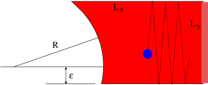
Figure 1: (Color online) Sketch of the billiard system of Eq. ​​(13). The unperturbed billiard is a rectangle of size $L_{x}\times L_{y}$. The deformation $U$, due to the radius of curvature $R$ of the left wall, is characterized by the parameter ${u=L_{y}/R}$. In order to break the mirror symmetry the center of the curved wall is shifted upwards a vertical distance ${\varepsilon}$. The time dependent perturbation is due to the displacement $f(t)$ of the right wall.

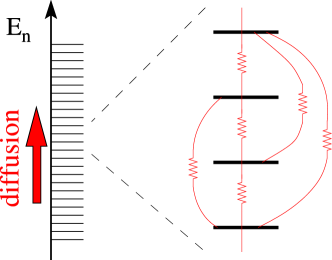
Figure 2: (Color online) The driving induces transitions between levels $E_{n}$ of a closed system, leading to diffusion in energy space, and hence an associated heating. The diffusion coefficient $D_{\mbox{\tiny E}}$ can be calculated using a resistor network analogy. Connected sequences of transitions are essential in order to have a non-vanishing result, as in the theory of percolation.

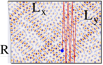
Figure 3: (Color online) An image of the eigenstate $E_{n}{\simeq}13618$ for the billiard of Fig. ​​1 with $L_{x}{=}1.5$, and $L_{y}{=}1.0$, and ${R{=}8}$, and ${\varepsilon=0.1}$. In the numerics the units are chosen such that $\hbar_{\mbox{\tiny Planck}}{=}1$ and the mass is $\mathsf{m}{=}1/2$.

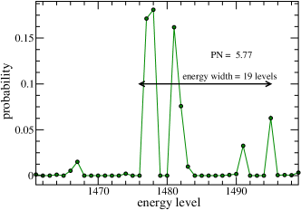
Figure 4: (Color online) Using a truncated matrix representation of the deformed billiard ${\mathcal{H}_{0}+U}$ in the unperturbed basis ${\bar{\bm{n}}=(n_{x},n_{y})}$ of the non-deformed rectangular billiard ${\mathcal{H}_{0}}$, we find a representative eigenstate $n_{0}$ of the former and plot $|\langle E_{\bar{\bm{n}}}|E_{n_{0}}\rangle|^{2}$ versus the running index $\bar{\bm{n}}$ of the ordered energies. The participation number (PN) of an eigenstate in this basis reflects how many energy levels were mixed due to the deformation $u$. Having PN${>}1$ indicates that our data is beyond the FOPT regime. For the displayed eigenstate $\mbox{PN}\approx 5.77$, while its energy width is $19$ levels. The billiard parameters are $R=8$ and $1/\hbar\approx 27.15$.

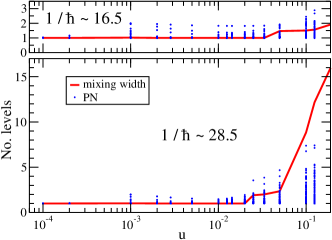
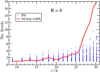
Figure 5: (Color online) The participation number (PN) of the eigenstates as a function of $u$ (panel a) and $\hbar$ (panel b). The parameter $\hbar$ characterizes an energy window that contains $\sim 100$ eigenstates. The method of calculation is as explained in Fig. ​​4. The average energy width in units of mean level spacing is represented by red solid line. Having average width larger than the average PN is an indication for sparsity.

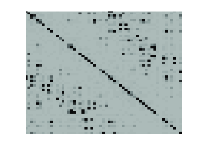
Figure 6: (Color online) Image of the perturbation matrix $\bm{X}=\{|F_{nm}|^{2}\}$ for the billiard of Fig. ​​3. within the energy window ${3500<E_{n}<4000}$. This matrix is sparse. More generally it might have some texture. The latter term applies if the arrangement of the large elements is characterized by some pattern.

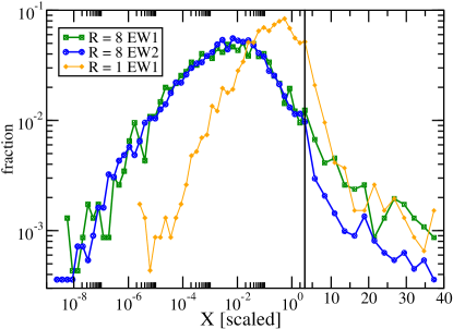
Figure 7: (Color online) Histogram of the values of the elements $X_{nm}$ that reside in the central band of the matrix. The analysis is done for the billiard of Fig. ​​3 where ${R=8}$. The statistics includes all the elements in the energy windows ${100<E<4000}$ (EW1), and ${10000<E<14000}$ (EW2). For sake of comparison we display results also for ${R=1}$.

a                           

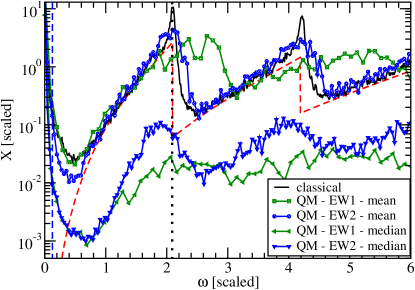
b                           

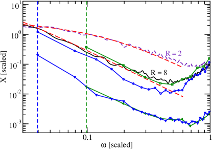
Figure 8: (Color online) The band profile of the perturbation matrix for the billiard of Fig. ​​3 where ${R=8}$. (a)  The algebraic average and median along the diagonals of the $X_{nm}$ matrix versus ${\omega\equiv(E_{n}{-}E_{m})}$. The vertical axis is normalized with respect to $C_{\infty}$, while the horizontal axis is $\omega/v_{\mbox{\tiny E}}$. The classical power spectrum is presented to demonstrate the applicability of the semiclassical relation Eq. ​​(27). The red line is the analytical expression that applies to zero deformation. The dotted vertical line is the frequency $1/t_{\mbox{\tiny L}}$ and the dashed one is $1/t_{\mbox{\tiny R}}$. (b)  Zoom of the $\omega\ll 1/t_{\mbox{\tiny L}}$ region. For sake of comparison we display results also for ${R=2}$. The vertical lines indicate the mean level spacing. The dashed red curves are based on Eq.(52).

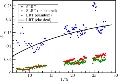
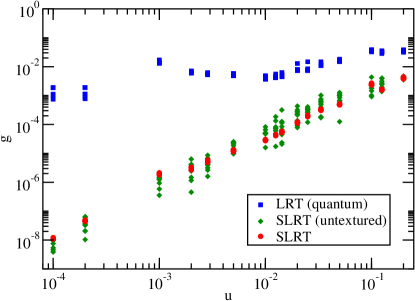
Figure 9: (Color online) SLRT vs LRT. The scaled absorption coefficient $g_{c}$ (LRT) and $g=g_{s}g_{c}$ (SLRT) versus the dimensionless $1/\hbar$ (upper panel), and versus the dimensionless deformation parameter ${u=L/R}$ (lower panel). Note that ${g=1}$ is the prediction of the “Wall formula”, while the line is based on the classical analysis. In the upper panel the analysis has been done for the billiard of Fig. ​​1. The calculation of each point has been carried out on a $100\times 100$ sub-matrix of $\bm{X}$ centered around the $\hbar$ implied energy $E$. The “untextured” data points are calculated for an artificial random matrices with the same bandprofile and sparsity (but no texture). The complementary lower panel is oriented to show the small $u$ dependence. The analysis is based on a truncated matrix representation of ${\mathcal{H}_{0}+U}$, within an energy window that corresponds to ${1/\hbar\sim 9}$. Due to the truncation there is some quantitative inaccuracy with regard to the larger $g$ values.

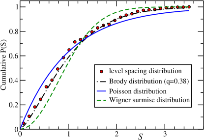
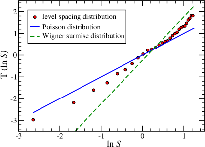
Figure 10: (Color online) (a) Cumulative histogram for the level spacing distribution $P(S)$ with fitting to Brody distribution ($q{=}0.38$), and contrasted with Poisson distribution ($q{=}0$) and the Wigner surmise ($q{=}1$). (b) The Brody parameter is determined via the slope of $T(x)$ as explained in the text.

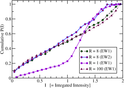
Figure 11: (Color online) Wavefunction intensity statistics: The cumulative distribution of the integrated intensity $I_{n}$ of Eq. ​​(94) is presented. As $R$ becomes larger the distribution further deviates from Gaussian statistics. The statistics includes all the eigenfunctions in the energy windows ${100<E<4000}$ (EW1), and ${10000<E<14000}$ (EW2).

References

- (1) M. Feingold, A. Peres, Phys. Rev. A 34 591, (1986).
- (2) M. Feingold, D. Leitner, M. Wilkinson, Phys. Rev. Lett. 66, 986 (1991).
- (3) M. Wilkinson, M. Feingold, D. Leitner, J. Phys. A 24, 175-182 (1991).
- (4) M. Feingold, A. Gioletta, F.M. Izrailev, L. Molinari, Phys. Rev. Lett. 70, 2936–2939 (1993).
- (5) T. Prosen and M. Robnik, J. Phys. A 26 L319 (1993)
- (6) T. Prosen, Ann. Phys. (N.Y.) 235, 115 (1994)
- (7) D.H.E. Gross, Nucl. Phys. A 240, 472 (1975).
- (8) J. Blocki, Y. Boneh, J.R. Nix, J. Randrup, M. Robel, A.J. Sierk, W.J. Swiatecki, Ann. Phys. 113, 330 (1978).
- (9) S.E. Koonin, R.L. Hatch, J. Randrup, Nuc. Phys. A 283, 87 (1977).
- (10) N. Friedman, A. Kaplan, D. Carasso, N. Davidson, Phys. Rev. Lett. 86, 1518 (2001).
- (11) A. Kaplan, M. Andersen, N. Friedman, N. Davidson, in Chaotic Dynamics and Transport in Classical and Quantum Systems, Editors: P. Collet, M. Courbage, S. Metens, A. Neishtast, G. Zaslavsky, NATO science series II, vol.182, p.239 (Springer 2004).
- (12) A. Kaplan, N. Friedman, M. F. Andersen, and N. Davidson, Phys. Rev. Lett. 87, 274101 (2001).
- (13) M. Andersen, A. Kaplan, T. Grunzweig and N. Davidson, Phys. Rev. Lett. 97, 104102 (2006).
- (14) A. Stotland, D. Cohen, N. Davidson, Europhys. Lett. 86, 10004 (2009).
- (15) L. A. Bunimovich, and Ya. G. Sinai, Comm. Math. Phys. 78, 479-497, 1981
- (16) L.-S. Young, Ann. of Math. 147(3), 585-650, 1998
- (17) B.J. Alder, T.E. Wainwright, Phys. Rev. A 1, 18 (1970).
- (18) F. Vivaldi, G. Casati, I. Guarneri, Phys. Rev. Lett. 51, 727 (1983).
- (19) G. Casati and T. Prosen, Phys. Rev. Lett. 85, 4261 (2000) M. Degli Esposti, S. O’Keefe and B. Winn, Nonlinearity 18, 1073 (2005).
- (20) E.B. Bogomolny, U. Gerland, C. Schmit, Phys. Rev. E 59, R1315 (1999).
- (21) A. Backer, R. Schubert, P. Stifter, J. Phys. A 30 6783 (1997).
- (22) F. Borgonovi, G. Casati and B. Li, Phys. Rev. Lett. 77, 4744 (1996).
- (23) K.M. Frahm and D.L. Shepelyansky, Phys. Rev. Lett. 78, 1440 (1997).
- (24) A. Stotland, L.M. Pecora and D. Cohen, Europhys. Lett. 92, 20009 (2010).
- (25) E.J. Austin, M. Wilkinson, Europhys. Lett. 20, 589 (1992).
- (26) T. Prosen, M. Robnik, J. Phys. A 26, 1105 (1993).
- (27) Y. Alhassid, R.D. Levine, Phys. Rev. Lett. 57, 2879 (1986).
- (28) Y.V. Fyodorov, O.A. Chubykalo, F.M. Izrailev, G. Casati, Phys. Rev. Lett. 76, 1603 (1996).
- (29) D. Cohen, T. Kottos, H. Schanz, J. Phys. A 39, 11755 (2006).
- (30) M. Wilkinson, B. Mehlig, D. Cohen, Europhys. Lett. 75, 709 (2006).
- (31) A. Stotland, T. Kottos, D. Cohen, Phys. Rev. B 81, 115464 (2010), and further references therein.
- (32) R. Ram-Mohan, Finite Element and Boundary Element Applications in Quantum Mechanics (Oxford University Press, Oxford, UK, 2002).
- (33) D. Cohen, Annals of Physics 283, 175 (2000).
- (34) A. Barnett, D. Cohen, E.J. Heller, Phys. Rev. Lett. 85, 1412 (2000);
- (35) A. Barnett, D. Cohen, E.J. Heller, J. Phys. A 34, 413 (2001).
- (36) For a review see “(Almost) everything you always wanted to know about the conductance of mesoscopic systems” by A. Kamenev and Y. Gefen, Int. J. Mod. Phys. B9, 751 (1995).
- (37) D. Cohen, A. Barnett, E.J. Heller, Phys. Rev. E 63, 46207 (2001).
- (38) A. Stotland, R. Budoyo, T. Peer, T. Kottos, D. Cohen, J. Phys. A (FTC) 41, 262001 (2008).
- (39) B.V.Chirikov, Phys. Rep. 52, 263 (1979).
- (40) S. Fishman, D.R. Grempel and R.E. Prange, Phys. Rev. Lett. 49, 509 (1982).
- (41) S. Fishman in ”Quantum Chaos”, Proceedings of the International School of Physics ”Enrico Fermi”, Course CXIX, Ed. G. Casati, I. Guarneri and U. Smilansky (North Holland 1991).
- (42) M. Raizen in ”New directions in quantum chaos”, Proceedings of the International School of Physics ”Enrico Fermi”, Course CXLIII, Edited by G. Casati, I. Guarneri and U. Smilansky (IOS Press, Amsterdam 2000).
- (43) F. Lenz, F.K. Diakonos, P. Schmelcher, Phys. Rev. Lett. 100, 014103 (2008); Europhys. Lett. 79, 2002 (2007).
- (44) I. Sela, J. Aisenberg, T. Kottos and D. Cohen, J. Phys. A (FTC) 43, 332001 (2010).
- (45) E. Ott, Phys. Rev. Lett. 42, 1628 (1979).
- (46) R. Brown, E. Ott, C. Grebogi, Phys. Rev. Lett. 59, 1173 (1987).
- (47) R. Brown, E. Ott, C. Grebogi, J. Stat. Phys. 49, 511 (1987).
- (48) C. Jarzynski, Phys. Rev. E 48, 4340 (1993).
- (49) C. Jarzynski, Phys. Rev. Lett. 74, 2937 (1995).
- (50) M. Wilkinson, J. Phys. A 21, 4021 (1988).
- (51) M. Wilkinson, E.J. Austin, J. Phys. A 28, 2277 (1995).
- (52) J.M. Robbins, M.V. Berry, J. Phys. A 25 L961 (1992).
- (53) D. Cohen, Phys. Rev. Lett. 82, 4951 (1999).
- (54) D. Cohen, T. Kottos, Phys. Rev. Lett. 85, 4839 (2000).
- (55) D.M. Basko, M.A. Skvortsov, V.E. Kravtsov, Phys. Rev. Lett. 90, 096801 (2003).
- (56) A. Silva, V.E. Kravtsov, Phys. Rev. B 76, 165303 (2007).
- (57) T. Prosen, D.L. Shepelyansky, Eur. Phys. J. B 46, 515 (2005).
- (58) M.V. Berry, Nonlinearity 1, 399 (1988)
a
b