Mass loss from inhomogeneous hot star winds

Abstract

Context. Mass loss is essential for massive star evolution, thus also for the variety of astrophysical applications relying on its predictions. However, mass-loss rates currently in use for hot, massive stars have recently been seriously questioned, mainly because of the effects of wind clumping.

Aims. We investigate the impact of clumping on diagnostic ultraviolet resonance and optical recombination lines often used to derive empirical mass-loss rates of hot stars. Optically thick clumps, a non-void interclump medium, and a non-monotonic velocity field are all accounted for in a single model. The line formation is first theoretically studied, after which an exemplary multi-diagnostic study of an O-supergiant is performed.

Methods. We used 2D and 3D stochastic and radiation-hydrodynamic wind models, constructed by assembling 1D snapshots in radially independent slices. To compute synthetic spectra, we developed and used detailed radiative transfer codes for both recombination lines (solving the ‘formal integral’) and resonance lines (using a Monte-Carlo approach). In addition, we propose an analytic method to model these lines in clumpy winds, which does not rely on optically thin clumping.

Results. The importance of the ‘vorosity’ effect for line formation in clumpy winds is emphasized. Resonance lines are generally more affected by optically thick clumping than recombination lines. Synthetic spectra calculated directly from current radiation-hydrodynamic wind models of the line-driven instability are unable to in parallel reproduce strategic optical and ultraviolet lines for the Galactic O-supergiant $\lambda$ Cep. Using our stochastic wind models, we obtain consistent fits essentially by increasing the clumping in the inner wind. A mass-loss rate is derived that is approximately two times lower than what is predicted by the line-driven wind theory, but much higher than the corresponding rate derived when assuming optically thin clumps. Our analytic formulation for line formation is used to demonstrate the potential importance of optically thick clumping in diagnostic lines in so-called weak-winded stars and to confirm recent results that resonance doublets may be used as tracers of wind structure and optically thick clumping.

Conclusions. We confirm earlier results that a re-investigation of the structures in the inner wind predicted by line-driven instability simulations is needed. Our derived mass-loss rate for $\lambda$ Cep suggests that only moderate reductions of current mass-loss predictions for OB-stars are necessary, but this nevertheless prompts investigations on feedback effects from optically thick clumping on the steady-state, NLTE wind models used for quantitative spectroscopy.

1 Introduction

Massive stars are fundamental in many fields of modern astrophysics. In the present Universe, they dynamically and chemically shape their surroundings and the interstellar medium by their output of ionizing radiation, energy and momentum, and nuclear processed material. In the distant Universe, they dominate the ultraviolet (UV) light from young galaxies. Indeed, massive stars may be regarded as ‘cosmic engines’ (Bresolin et al., 2008). Hot, massive stars possess strong and powerful winds that affect evolutionary time scales, chemical surface abundances, and luminosities. In fact, changing the mass-loss rates of massive stars by only a factor of two has a dramatic effect on their overall evolution (Meynet et al., 1994). The winds from these stars are described by the radiative line-driven wind theory, in which the standard model (based on the pioneering works by Lucy & Solomon, 1970; Castor et al., 1975) assumes that the wind is stationary, spherically symmetric, and homogeneous. Despite this theory’s apparent success (e.g., Vink et al., 2000), theoretical as well as observational evidence of an inhomogeneous, time-dependent wind has become overwhelming in the past years (for a comprehensive summary, see Puls et al., 2008).

Direct simulations of the time-dependent wind have confirmed that the so-called line-driven instability causes a highly structured wind in both density and velocity (Owocki et al., 1988; Feldmeier, 1995; Dessart & Owocki, 2005). Much indirect evidence of such small-scale inhomogeneities (clumping) has arisen from quantitative spectroscopy. Clumping has severe consequences for any interpretation of observed spectra, with the inferred mass-loss rates particularly affected. When deriving mass-loss rates from observations, wind clumping has traditionally been accounted for by assuming optically thin clumps and a void interclump medium, while keeping a smooth velocity field. Results based on this microclumping approach have, for example, led to a downward revision of empirical mass-loss rates from Wolf-Rayet (WR) stars by roughly a factor of three (reviewed in Crowther, 2007).

However, for O stars, highly clumped winds with very low mass-loss rates must be invoked in order to reconcile investigations of different diagnostics within the microclumping model. The most alarming example was the phosphorus v (Pv) UV analysis by Fullerton et al. (2006), which indicated reductions of previously accepted values by an order of magnitude (or even more), with dwarfs, giants, and supergiants all affected (but see also Waldron & Cassinelli 2010, who argued that xuv radiation could seriously alter the ionization fractions of Pv). Such low mass-loss rates would be in stark contrast with the predictions of line-driven wind theory and have dramatic consequences for the evolution of, and feedback from, massive stars. Naturally, the widely discrepant values inferred from different observations and diagnostics drastically lower the reliability of mass-loss rates currently in use, and an explanation is urgently needed. A key question is whether the microclumping model fails to deliver accurate empirical rates under certain conditions.

Simplified techniques to account for optically thick clumps in X-ray line formation have been developed (Feldmeier et al., 2003; Owocki et al., 2004), but it has yet to be settled whether or not this is important to consider when deriving empirical mass-loss rates from these diagnostics (Oskinova et al., 2006; Cohen et al., 2010). First attempts to relax the assumptions of the microclumping model for UV resonance lines were made by Oskinova et al. (2007) (optically thick clumps), Zsargó et al. (2008) (a non-void interclump medium), and Owocki (2008) (a non-monotonic velocity field). Sundqvist et al. (2010) (hereafter Paper I) carried out the first detailed investigation, relaxing all the above assumptions, and showed that, indeed, the microclumping approximation is not a suitable assumption for UV resonance line formation under conditions prevailing in typical OB-star winds. Recently, these results were empirically supported for the case of B supergiants by Prinja & Massa (2010), who analyzed profile-strength ratios of the individual components of resonance line doublets and found that the observed ratios were inconsistent with lines formed in a smooth or ‘microclumped’ wind. Furthermore, Paper I demonstrated that resonance line profiles calculated from 2D, stochastic wind models were compatible with mass-loss rates an order of magnitude higher than those derived from the same lines but using the microclumping technique. However, as pointed out in that paper, a consistent modeling of the resonance lines also introduces degeneracies among the parameters used to define the wind structure, degeneracies that can only be broken by considering different diagnostics (depending on different parameters) in parallel.

Here we make a first attempt toward such multi-diagnostic studies. We extend our 2D wind models from Paper I to 3D, and relax the microclumping approximation also for the optical mass loss diagnostics H_α and He ii 4686 $\rm\AA$ (Sect. 2). In Sect. 3 we theoretically investigate H_α and resonance line formation in clumpy winds, and propose an analytic treatment of the lines that does not rely on the microclumping approximation. A simultaneous optical and UV diagnostic analysis is carried out in Sect. 4 for the Galactic O6 supergiant $\lambda$ Cep, using time-dependent radiation-hydrodynamic (RH) models as well as stochastic ones together with our new tools for the radiative transfer in clumped winds. These results are discussed in Sect. 5, while two initial applications of our analytic formulation are given in Sect. 6. We summarize the paper and outline future work in Sect. 7.

2 Wind models and radiative transfer

Table 1: Parameters for the time-dependent RH model of $\lambda$ Cep (see text).

Name	Parameter	Value
Spectral type		O6 I(n) fp
Effective temperature	$T_{\rm eff}$	36 000 K
Stellar radius	$R_{\star}$	21.1 $R_{\odot}$
Surface gravity	$\log g$	3.55
Stellar luminosity	$\log L/L_{\odot}$	5.83
Terminal speed	$\varv_{\infty}$	2200 $\rm km\,s^{-1}$
Mass-loss rate	$\dot{M}$	$1.5\,\times$ $10^{-6}\,{\rm M_{\odot}/yr}$
Helium abundance	$Y_{\rm He}\equiv n_{\rm He}/n_{\rm H}$	0.1
CAK exponent	$\alpha_{\rm CAK}$	0.7
Initial Langevin	$\varv_{\rm turb}/\varv_{\rm sound}$	0.5
turbulence fluctuation

We create 2D and 3D RH and stochastic wind models by assembling snapshots in radially independent wind slices (see Sect. 2.3).

Table 1 summarizes properties of a time-dependent RH model computed following the approach in Feldmeier et al. (1997), which introduces base perturbations from Langevin turbulence into an unstable line-driven wind. The line force is computed with the nonlocal ‘Smooth Source Function’ (SSF; Owocki & Puls, 1996) method that allows one to follow the nonlinear evolution of the strong, intrinsic line-deshadowing instability, while also accounting for the diffuse line drag (Lucy, 1984) that reduces (and even eliminates) the instability near the wind base. The net result is a highly structured wind characterized by high-speed rarefactions and slower, dense clumps (actually shells in these 1-D simulations). In comparison to self-excited instability simulations (e.g., Runacres & Owocki, 2002), the base perturbations here induce a somewhat lower onset and greater velocity dispersion of the wind clumping. A central goal here is to examine the effects of this extensive structure on wind diagnostics. Stellar and wind parameters are taken from Repolust et al. (2004), except for the mass-loss rate (see Sect. 4).

Basic assumptions of our empirical, stochastic models were described in detail in Paper I. Essentially, they are constructed so to resemble the main structures predicted by the RH simulations, while still allowing for a variation in the key parameters controlling the line formation (see below).

2.1 Parameters describing a structured wind

Table 2: Basic structure parameters defining a stochastic wind model.

Name	Parameter
Clumping factora	$f_{\rm cl}$
Average time interval	$\delta t$
between release of clumps
Interclump medium density parameter	$x_{\rm ic}$
Velocity span of clump	$\delta\varv$
a $f_{\rm cl}$ may be replaced by the volume filling factor $f_{\rm v}$.
The two are related via $x_{\rm ic}$ (see Paper I).

When creating our stochastic wind models, we take an heuristic approach and use a set of parameters to define the structured medium. The clumping factor $f_{\rm cl}$($\varv$) $\equiv\langle\rho^{2}\rangle/\langle\rho\rangle^{2}$, with the angle brackets denoting spatially averaged quantities, is the only necessary structure parameter when calculating spectra via the microclumping technique. Microclumping gives rise to the well known result that the opacities for processes that depend on the square of the density (for example H_α emission in OB-stars) are augmented by $f_{\rm cl}$ as compared to a smooth model with the same mass-loss rate; in contrast, opacities for processes that depend linearly on the density (for example the uv resonance lines) are not directly affected. Thus, if the wind is clumped, mass-loss rates derived from smooth models applied to H_α are overestimated by a factor of $\sqrt{f_{\rm cl}}$. In addition, the occupation numbers are modified for all diagnostics because of the changed rates in the statistical equilibrium equations. For a comprehensive discussion on the effects of microclumping on various diagnostics, see Puls et al. (2008).

If the assumptions behind the microclumping model are not satisfied (e.g. if clumps are optically thick for the investigated diagnostic), the line formation will depend on more structure parameters than just $f_{\rm cl}$. Thus, relaxing the microclumping approximation means that we must consider additional parameters when describing the structured wind. These parameters (for a two component medium) were defined and discussed in Paper I, and are listed in Table 2. We stress that they are essential for the radiative transfer in an inhomogeneous medium, and not merely ‘ad-hoc parameters’ used in a fitting procedure.

In addition to the clumping factor $f_{\rm cl}$ (or alternatively $f_{\rm v}$), $x_{\rm ic}$ $\equiv\rho_{\rm ic}/\rho_{\rm cl}$ denotes the density ratio of the interclump (ic) to clumped (cl) medium. The time interval $\delta t$ (given in units of the wind’s dynamic time scale, $R_{\star}$/$\varv_{\infty}$, and not necessarily constant throughout the wind) effectively sets the physical distances between clumps, also known as the porosity length $h$ (Owocki et al., 2004), which in our geometry is given by $h=\varv_{\beta}\delta t$. Moreover, assuming a smooth underlying field of customary $\beta$-type, $\varv_{\beta}(r)=\varv_{\infty}(1-b/r)^{\beta}$ with $b$ set by the assumed velocity at the wind base $\varv_{\rm min}=\varv(r=1)$, this time interval sets the velocity separation between the clumps $\Delta\varv\approx\varv_{\beta}\delta td\varv_{\beta}/dr$ (Appendix A). Finally, the ratio of the clump velocity span $\delta\varv$ (as defined in Fig. 2 in Paper I) to this velocity separation (representing a velocity filling factor, see Appendix A) largely controls how strongly a perturbed velocity field affects line formation. In addition to these basic parameters, the velocity $\varv_{\rm cl}$ (or radius $r_{\rm cl}$) at which clumping is assumed to start also plays an important role for the line formation. Note also that the parameters defining these stochastic winds are independent of the physical origin to the inhomogeneities.

The stochastic models should be distinguished from the time-dependent RH simulations. In the latter the structure arises naturally from following the time evolution of the wind and stems directly from the line-driven instability. Thus, the time-averaged structure parameters, as functions of radius, are an outcome of these simulations (in contrast to the stochastic models, where they are used as fundamental parameters defining the structured wind). Nonetheless, the exact wind structure still depends on the chosen initial conditions, for example on whether the instability is self-excited or triggered by some excitation mechanism (the latter is done here, see Table 1). Finally, as shown in Paper I, by choosing a suitable set of structure parameters one can reconcile spectrum synthesis results stemming from the stochastic models with those from RH simulations.

2.2 Radiative transfer

For resonance lines we use the Monte-Carlo code described in Paper I, but a new radiative transfer code has been developed for the synthesis of wind recombination lines presented here. We investigate the O star recombination lines H_α and He ii 4686. Recall that recombination lines and resonance lines are formed differently. First, the optical depths are calculated in different ways. For resonance lines, the optical depths may be computed via a line-strength parameter, $\kappa_{0}$, which is assumed to be constant throughout the wind and is proportional to the product of the mass-loss rate and the abundance (by number), $\alpha_{\rm i}\equiv n_{\rm i}/n_{\rm H}$, of the considered element $i$. $\kappa_{0}$ may be expressed as (e.g., Puls et al., 2008)

$$\kappa_{0}=\frac{\dot{M}}{R_{\star}\varv_{\infty}^{2}}\frac{\pi e^{2}/m_{\rm e}c}{4\pi m_{\rm H}}\frac{\alpha_{\rm i}}{1+4Y_{\rm He}}f_{\rm lu}\lambda_{0},$$ (1)

where $e$ and $m_{\rm e}$ are the electron charge and mass, respectively, $c$ the speed of light, $m_{\rm H}$ the atomic hydrogen mass, $Y_{\rm He}$ the helium abundance, $f_{\rm lu}$ the transition’s oscillator strength, and $\lambda_{0}$ its rest wavelength. The advantage with this definition is that the radial Sobolev optical depth in a smooth wind collapses to

$$\tau_{\rm Sob}=q\frac{\kappa_{\rm 0}}{r^{2}\varv{\rm d}\varv/{\rm d}r},$$ (2)

where $q$ is the ionization fraction of the considered ion, and $r$ is measured in units of $R_{\star}$ and $\varv$ in units of $\varv_{\infty}$.

For H_α, the analog to $\kappa_{0}$ is the parameter $A$ (Puls et al., 1996, Eqs. 1-3). $A$ is proportional to the mass-loss rate squared and to the NLTE departure coefficient, $b_{\rm i}$, of the lower transition level (minus the correction factor for stimulated emission). $b_{\rm i}=n_{\rm i}/n_{\rm i}^{\rm*}$, where $n_{\rm i}^{*}$ is the occupation number of level $i$ in LTE with respect to the ground state of the next ionization state. In this case, the radial Sobolev optical depth in a smooth wind becomes (Puls et al., 1996)

$$\tau_{\rm Sob}=\frac{A(r)}{r^{4}\varv^{2}d\varv/dr}.$$ (3)

In addition to their different optical depths, recombination lines are (mainly) formed by recombining ions creating wind photons, whereas resonance lines are formed by re-distributing photospheric stellar continuum radiation by line scattering. Therefore the participating atomic levels for recombination lines are rather close to LTE with respect to the next ionization state (see Fig. 5), which means that the departure coefficients and thereby also the line source function, $S_{\rm l}\propto(e^{h\nu/kT}b_{\rm l}/b_{\rm u}-1)^{-1}$, for these lines are basically unaffected by the radiation field and its dilution. In turn this allows us to prescribe the source functions (Puls et al., 1996, 2006) and simply carry out the ‘formal integrals’ within our stochastic and RH winds. In the present work, we assume that changes in the NLTE departure coefficients due to optically thick clumps can be neglected for recombination-based line formation, and simply calculate the $b_{\rm i}$’s from NLTE model atmospheres using the microclumping approximation. Taking the example of H_α in O stars, this assumption should be reasonable, for the H_α departure coefficients in this domain are very close to unity and the ionization of hydrogen is complete. However, for the case of, e.g., A-supergiants, the assumption no longer holds, because in that stellar domain H_α’s lower level becomes the effective ground state of hydrogen, which means that the line transforms to a quasi-resonance line (and thereby that $S_{\rm l}$ depends on the radiation field, Puls et al. 1998).

As described in Paper I, also the ionization fractions $q$ for resonance line formation are calculated assuming microclumping. These fractions are used both within clumps and for the interclump medium. The potential feedback effects of optically thick clumping on the departure coefficients and ionization fractions will be investigated by incorporating the analytic methods developed in Sect. 3 into suitable NLTE atmosphere codes, and reported in a future paper.

The assumption of prescribed departure coefficients is an enormous simplification compared to the UV resonance lines, and has enabled us to extend our 2D wind models to 3D when modeling recombination lines. In the synthesis we follow the basic method introduced by Puls et al. (1996), which does not rely on the Sobolev approximation, with appropriate modifications for the line opacities of He ii 4686. A core/halo approach is adopted, in which a photospheric profile is used as a lower boundary input (at $r=1$, with $r$ in units of the stellar radius) and the radiative transfer is solved only in the wind. As for the resonance lines (Paper I), we assume pure Doppler line broadening within the wind, characterized by a thermal speed, $\varv_{\rm t}$, given throughout the paper in units of $\varv_{\infty}$.

Our new recombination line code has been extensively tested and showed to yield equivalent results with Puls et al. (2006) for smooth winds. Also, results based on the microclumping technique are reproduced for stochastic as well as RH winds with low wind densities, as expected because the clumps then remain optically thin. In our applications, we use hydrogen and helium occupation numbers calculated by fastwind model atmospheres (Puls et al., 2005), under the microclumping approximation, as input for the radiative transfer to compute synthetic spectra. Photospheric profiles are taken from NLTE calculations of atmospheres with negligible winds. The consistency between unified (meaning a simultaneous treatment of the photosphere and wind) model atmosphere calculations and the simplified core/halo approach has been verified in the microclumping limit, for recombination lines as well as for resonance lines. Moreover, we have found that averaged recombination line profiles calculated from our earlier 2D, stochastic models are almost identical to those calculated from our new 3D ones, as was already anticipated for the UV resonance lines in Paper I.

The He ii blend in H_α.

The star’s helium abundance has of course been considered in the calculation of the H_α wind opacity, but for simplicity we include the He ii blend only in the photospheric profile, thus neglecting its direct contribution to the wind emission. This results in a slight underestimate of the total wind opacity of the line complex. However, by comparing to unified model atmosphere calculations that consistently treat the He ii blend, we have found that the direct helium contribution is low for our typical stars of interest, and in our applications for $\lambda$ Cep it can even be neglected. Although sufficient for our purposes here, this approach should obviously not be generalized, because it may yield unrealistic results for stars with parameters different from our template star.

2.3 Geometry

To construct (pseudo-)3D winds, we use the ‘patch method’ from Dessart & Owocki (2002). A standard right-handed spherical system ($r,\Theta,\Phi$) is used, defined relative to a Cartesian set ($X,Y,Z$). However, when computing recombination lines, we no longer assume symmetry in the azimuthal ($\Phi$) direction (as was done in Paper I). The lateral scale of coherence in the wind is set by the parameter $N_{\Theta}$ and by assuming that the physical coherence lengths in both lateral directions are approximately equal (Fig. 1). This assumption is reasonable because, within our approach, which for example does not include an axis of rotation, all observer directions should be alike. Thus, if we desire a coherence scale of 3 degrees, the number of slices in the polar direction should be $N_{\Theta}=180/3=60$ and in the azimuthal direction $N_{\Phi}=\rm int$$[2N_{\Theta}\sin\Theta]$, i.e., $2N_{\Theta}$ at the equator but fewer toward the pole in order to preserve the physical length scales. Wind slices are then assigned randomly from a large number of spherically symmetric simulations (either RH or stochastic).

$N_{\Theta}$ thus enters all our models as an input parameter. Paper I showed that this parameter does not change the strengths of the resonance lines. More tests have shown that also the effects on recombination lines are modest for investigated values. Therefore all 3D models in this paper assume $N_{\Theta}=60$, meaning a coherence length of 3 degrees at the equator, which is consistent with observational constraints derived from line-profile variability analysis (Dessart & Owocki, 2002). Theoretical constraints on $N_{\Theta}$ are still lacking, and will require a careful treatment of the lateral radiation transport in RH models. The first 2D simulations by Dessart & Owocki (2003) neglected this transport and resulted in a laterally fragmented wind down to the grid scale but the follow-up study (Dessart & Owocki, 2005) included a simplified 3-ray approach and resulted in larger (but un-quantified) lateral coherence scales.

For recombination line formation, the observer is assumed to be located at infinity in the $Z_{\rm u}$ (subscript u denoting a unit vector) direction. The geometry is sketched in Fig. 1. We solve the radiative transfer using a traditional $(P,Z)$ system for a set of P-rays, each defined by the minimum radial distance to the $Z$ axis and by the azimuthal angle $\Phi$, which is constant along a given ray. If the angle between the ray and the radial coordinate is $\theta$, then $\mu=\cos\theta$ and $P=r\sqrt{1-\mu^{2}}$. Thus, for rays in direction $Z_{\rm u}$ the radiation angle $\theta$ coincides with the polar coordinate $\Theta$, and it becomes trivial to calculate the physical locations at which wind-slice borders are crossed. The observed flux may then finally be computed by performing a double integral of the emergent intensity over $P$ and $\Phi$.

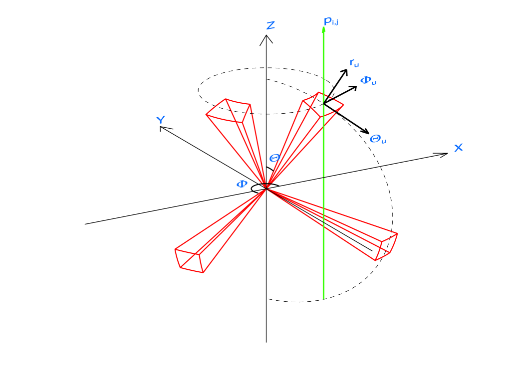
Figure 1: Illustration of the wind geometry, see text. A color version of this figure is available in the web version.

3 Theoretical considerations of resonance and recombination line formation in clumpy winds

Resonance line formation in clumpy hot star winds was discussed in detail in Paper I. There we identified an intrinsic coupling between the effects of porosity and vorosity (=’velocity porosity’, Owocki, 2008), which we here further elaborate upon. In particular, we propose an analytic formulation of line formation in clumped hot star winds (that does not rely on the microclumping approximation). As already mentioned in Sect. 2, the development of such simplified approaches is important for properly including effects of optically thick clumping into atmospheric NLTE codes. For recombination lines, we focus on H_α and discuss impacts from optically thick clumping on its formation, using our stochastic wind models as well as an extension of the analytic treatment developed for the resonance lines.

3.1 Analytic treatment of resonance lines in clumpy winds

Figure 2: Panel a: $\xi$ (Eq. 5) as a function of wind velocity. Panel b: The relative contributions to $\xi$ from $f_{\rm vel}$ and $C\eta$. Curves in panels $a$ and $b$ have been calculated with $\kappa_{0}=5$ and thermal speed $\varv_{\rm t}=0.005$ (in units of $\varv_{\infty}$). Panels c and d: Analytic (Eq. 4, solid lines) and Monte-Carlo (dashed lines) based absorption part resonance line profiles from clumped winds, as compared to smooth results (dotted lines). Clumping starts at $\varv_{\rm cl}=0.2$ ($r_{\rm cl}=1.24$). Panel c: Profiles for three different values of the line strength $\kappa_{0}$ (indicated in the figure), with increased absorption for higher values of $\kappa_{0}$. Only the $\kappa_{0}=1$ profile is not saturated (i.e., does not display $R_{\rm a}=0$) for smooth models. Panel d: Profiles for $\kappa_{0}=5$ and different values of $\varv_{\rm t}$, as indicated in the figure. No Monte-Carlo profile for the $\varv_{\rm t}=0$ case is shown (simply because we have not yet developed a ‘Sobolev version’ of this code). Analytic and Monte-Carlo profiles display increased absorption for higher values of $\varv_{\rm t}$, whereas all smooth profiles have $R_{\rm a}=0$.

Throughout this section we assume a smooth velocity field, characterized by $\beta=1$ (Sect. 2.1). Despite this, the vorosity effect will be demonstrated to be important for the line formation (i.e., a non-monotonic velocity field is not required for vorosity to be at work). Adopting the normalized, dimensionless frequency $x=(c/\varv_{\infty})(\lambda_{0}-\lambda)/\lambda$, and following the basic arguments of Owocki (2008), we write the absorption part of a normalized resonance line profile, $R_{\rm a,x}$, from a radial ray as (see Appendix A)

$$R_{\rm a,x}=\xi_{\rm x}e^{-\tau_{\rm cl,x}}+(1-\xi_{\rm x})e^{-\tau_{\rm ic,x}}.$$ (4)

$R_{\rm a,x}$ describes the part of the profile that stems from absorption of continuum photons released from the photosphere. The total line profile is given by $R_{\rm x}=R_{\rm a,x}+R_{\rm em,x}$, where $R_{\rm em,x}$ is the re-emission profile. The scattering nature of the resonance line source function significantly complicates the formation of $R_{\rm em,x}$. Therefore, for now we restrict ourselves to discussing $R_{\rm a,x}$ from a radial ray for these lines. For recombination lines, on the other hand, we will lift these restrictions and treat the complete line profile (Sect. 3.2). Obviously this must be done also for resonance lines before, e.g., including our analytic formalism in NLTE model atmosphere codes (see also Sect. 6.2). In any case, recall that $R_{\rm a,x}$ controls the actual line-profile strengths of resonance lines, because these are pure scattering lines formed out of re-distributed continuum radiation emerging from the photosphere.

In Eq. 4 we define $\xi$ as the fraction of the velocity field over which photons may be absorbed by clumps, with the $\tau$’s representing the optical depths for the clumped (subscript cl) and rarefied (subscript ic) regions. $\xi$ describes the essential effects of Owocki’s vorosity; the first term in Eq. 4 handles the part of the line profile emerging from absorption within the clumps, whereas the second term handles the part emerging from absorption within the interclump medium. What remains then is finding an appropriate expression for $\xi$. In Appendix A we argue that a reasonable approximation may be

$$\xi_{\rm x}\approx\frac{\delta\varv}{\Delta\varv}+C\frac{\varv_{\rm t}}{\Delta\varv}=f_{\rm vel}(\varv)+C(\varv)\eta(\varv),$$ (5)

with $\Delta\varv$ the velocity gap between two clump centers, $f_{\rm vel}$ the velocity filling factor (defined in full analogy with the traditional volume filling factor), $\eta$ the effective escape ratio (here re-defined from Paper I, see Appendix A), and $C$ a correction factor that depends on the line strength. The condition for interaction for a radial line photon is in the Sobolev approximation simply $x=\varv$, and, for simplicity, we from now on suppress all velocity dependencies of the quantities in Eq. 5. As shown in Appendix A, we may write

$$f_{\rm vel}=f_{\rm v}|\frac{\delta\varv}{\delta\varv_{\beta}}|,\qquad\eta=\frac{L}{h},$$ (6)

where $h$ is the porosity length of the medium and $L=\varv_{\rm t}/(d\varv/dr)$ the (in this case radial) Sobolev length. For the smooth velocity field considered in this section, $\delta\varv=\delta\varv_{\beta}$, which gives $f_{\rm vel}$=$f_{\rm v}$. Even though the principle effect of the optically thick clumps on resonance line formation is a velocity effect governed by $f_{\rm vel}$, Eqs. 4-6 indicate there is also a dependence on spatial porosity through the ratio $\eta=L/h$. This coupling was argued for already in Paper I. However, it appears that $\xi$ better characterizes the effects of clumping in resonance line formation than did our previous parametrization (see Appendix A). The optical depths entering Eq. 4 may be approximated by the corresponding Sobolev ones, corrected for the influence of $\eta$ (Appendix A). Then for resonance lines, $\tau_{\rm cl,x}\approx\tau_{\rm sm,x}/\xi_{\rm x}$ and $\tau_{\rm ic,x}=\tau_{\rm cl,x}x_{\rm ic}$, where $\tau_{\rm sm,x}$ is given by Eq. 2. Note that all parameters used to define our stochastic wind models (Table 2) enter the expression for $R_{\rm a,x}$, illustrating that indeed all these are important for the general line formation problem.

The upper two panels of Fig. 2 plot $\xi$ as well as the relative contributions from $f_{\rm vel}$ and $C\eta$ for a resonance line with line-strength parameter $\kappa_{0}=5$. We do not allow for $\xi$ values above unity (important for the outer wind, see also Appendix A), and we also recover the smooth result for velocities lower than $\varv_{\rm cl}$ simply by setting $\xi_{\rm x\leq\varv_{\rm cl}}=1$. All models displayed in Fig. 2 were calculated with density structure parameters $f_{\rm cl}$=4.0, $\delta t$=0.5, and $x_{\rm ic}$=0.0025. For a smooth model (with ionization fraction $q=1$, assumed in this section), $\kappa_{0}=5$ results in a profile at the saturation threshold. In the lower two panels we show analytic absorption-part line profiles calculated using Eq. 4 and profiles calculated using our Monte-Carlo code. To make consistent comparisons between methods, we accounted only for radial photons in the Monte-Carlo simulations. The agreement between the methods is very good, lending support to the proposed analytic treatment and providing a relatively simple explanation for the basic features of the synthetic profiles.

Evidently, profile-strength reductions can be quite dramatic for ‘moderately strong’ cases such as $\kappa_{0}=5$. For the very strong $\kappa_{0}=500$ line also the interclump medium is optically thick and the profiles are therefore saturated (which is a necessity because such saturated profiles are observed in hot stars). Note that, if $\delta\varv$ were much higher than $C\varv_{\rm t}$, one could neglect the second term in Eq. 5 and $\xi$ would become independent of the porosity length. If one also neglects the interclump medium (setting $x_{\rm ic}$=0), and assumes that clumps are optically thick throughout the entire wind (appropriate for the $\kappa_{0}=5$ line), then the observer in our example would simply receive a constant residual flux $R_{\rm a,x}=1-f_{\rm v}=0.75$. Fig. 2d shows that this generally does not hold (even for the idealized case of zero thermal speed, the interclump medium still plays a role), demonstrating that, along with the velocity filling factor $f_{\rm vel}$, in general both $x_{\rm ic}$ and $\eta$ also help shape the emergent profile for a wide range of line strengths and structure parameters. Fig. 2d illustrates the importance of accounting for the finite line profile width. $C\eta$ may not be neglected, even in models with very low, but finite thermal velocity, and becomes particularly important toward the blue edge of the line profiles. This occurs because the resonance zones in the outermost wind become very radially extended. $L$ thus grows whereas the distances between the clumps (determining $h$) are unaffected due to the very slowly changing velocity field. Consequently $\eta$ becomes very high and $\xi$ eventually reaches unity. Since the smooth $\kappa_{0}=5.0$ line is optically thick, a ‘blue absorption dip’ (extensively discussed in Paper I) is created.

Randomization effects are here neglected because we have used a smooth velocity field. When clumps are allowed to have velocities higher and lower than those given by the mean velocity field, overlapping velocity spans of the clumps lead to increased escape of photospheric photons. The blue absorption dip then becomes less prominent than what is displayed in Fig. 2, as discussed in Paper I (see also Appendix A, for some comments on randomization effects).

Nevertheless, this section demonstrates that the microclumping approximation can result in large errors if indeed the wind is clumped but the clumps are not optically thin. First applications of the analytic formulation are given in Sect. 6, for diagnostics of weak wind stars and for the predicted profile-strength ratios in resonance line doublets.

3.2 Recombination lines in clumpy winds

Figure 3: Upper panel: Deviations from the microclumping approximation of equivalent widths of synthetic H_α  line profiles versus mass-loss rate (see text). Clumping starts at $\varv_{\rm cl}=0.24$ and 0.06 ($r_{\rm cl}=1.3$ and 1.05), respectively, as indicated in the figure. Lower panel: H_α line profiles as calculated by stochastic, analytic, and microclumped models with $f_{\rm cl}$=9 and $\dot{M}$=10 $\times$ $10^{-6}\,{\rm M_{\odot}/yr}$, and the rest of the stellar and wind parameters as for $\lambda$ Cep. Clumping for all models starts at $\varv_{\rm cl}=0.24$.

We now leave the resonance lines behind and turn to the formation of recombination lines. We focus on H_α, the primary spectroscopic mass-loss diagnostic for O stars. He ii 4686 reacts similarly as H_α to clumping in our primary stars of interest (because He iii is the dominant ion in the line forming regions), and will be considered only in our diagnostic study of $\lambda$ Cep (Sect. 4).

First we present results from calculating H_α line profiles using our stochastic 3D wind models. Our main interest is to investigate differences with respect to the microclumping model, so main results are provided in terms of the deviation of the equivalent widths $W_{\lambda}$ between the two methods, $(W_{\lambda,\rm mic}-W_{\lambda})/W_{\lambda,\rm mic}$, as a function of mass-loss rate (here $W_{\lambda,\rm mic}$ denotes $W_{\lambda}$ as calculated from a model assuming microclumping). All models discussed in this section were calculated with unity departure coefficients, wind electron and radiation temperatures as for approximately $\lambda$ Cep (calibrated using unified NLTE model atmospheres, see Puls et al., 2006), and no input photospheric absorption profiles. We used structure parameters $f_{\rm cl}$=9.0, $\delta t$=0.5, $x_{\rm ic}=0.0025$, and a smooth velocity field characterized by $\beta=1$.

For typical O-supergiants, the equivalent widths of profiles calculated from stochastic models are slightly lower than those based on the microclumping technique (Fig. 3). Deviations stem from optically thick clumps. The dominating effect is on the wind emission of H_α photons rather than on the wind absorption of photospheric photons (in contrast to resonance lines, see previous section). This is because the source function for recombination lines is basically unaffected by the dilution of the radiation field, which for relatively strong and hot winds make these lines appear in emission and thereby suffer the main effect from a clumped wind on the emission part of the line profile. Moreover, the $\rho^{2}$-dependence of recombination line opacity increases the contrast between the optical depths for the clumps and those for the interclump medium, as compared to resonance line formation. This lowers the significance of the interclump medium and also causes the clump optical depths to decrease faster for increasing radii. The latter effect results in clumps that are optically thick only in the lower wind regions. Deviations from the microclumping limit are therefore more significant for cases with earlier onset of clumping. For example, the equivalent widths for the models with $\dot{M}$=2.5 $\times$ $10^{-6}\,{\rm M_{\odot}/yr}$ are reduced by 7 % and 17 % when clumping starts at $\varv_{\rm cl}=0.24$ and $\varv_{\rm cl}=0.06$, respectively. The effect is thus modest, but noticeable. Remember that reductions are measured against models assuming microclumping; the profiles are still much stronger than profiles computed from smooth models with the same mass-loss rate.

Our tests show that effects are confined to the line core and that the microclumping approximation provides accurate results in the line wings. However, Fig. 3 reveals prominent emission strength reductions for stronger winds, since then optical depth effects become important for ever larger portions of the total wind volume. Furthermore, the onset of clumping is irrelevant in these strong winds because the majority of the emission emerges from radii greater than $r_{\rm cl}$. This insensitivity to the onset of clumping also recovers the scaling invariant for microclumped winds ($\propto\sqrt{f_{\rm cl}}\dot{M}$, see Sect. 2.1). For typical OB-supergiants, however, this scaling does not hold because of the strong opacity contrast between wind radii lower than and greater than $r_{\rm cl}$. Very strong recombination lines, such as those displayed in Fig. 3 (lower panel), are typically seen in WR stars, for which however also a reduced hydrogen content is expected (as well as a breakdown of our assumption of an optically thin continuum). Nonetheless, our analysis could, of course, be generalized to recombination lines of other chemical species (as has been done for He ii 4686 in our application to $\lambda$ Cep), and may point to significant optical depth effects in the strong emission peaks of stars with very high mass-loss rates. Indeed, lower emission peaks in the theoretical spectrum of a WR star have been found by Oskinova et al. (2007), on the basis of scaling smooth opacities using a porosity formalism. However, when deriving empirical mass-loss rates from microclumping models of WR stars one normally considers also the electron scattering wings (which are unaffected by microclumping, see Hillier, 1991), and because clumps in these probably are optically thin it may be that lower emission peaks would have a greater effect on the inferred clumping factors than on the mass-loss rates.

Analytic treatment of recombination lines.

We can understand the reduction in H_α emission strengths using the same analytic treatment as outlined for resonance lines. Better yet, because the source function $S$ is almost unaffected by the radiation field (see Sect. 2), we can for recombination lines simulate the total profile, $R_{\rm x}=R_{\rm a,x}+R_{\rm em,x}$, writing

$$R_{\rm em,x}=S\xi_{\rm x}(1-e^{-\tau_{\rm cl,x}})+S(1-\xi_{\rm x})(1-e^{-\tau_{\rm ic,x}}),$$ (7)

where $S$ is given in units of the continuum intensity and evaluated at the resonance point. $R_{\rm em,x}$ is much more influenced by non-radial photons than is $R_{\rm a,x}$, so accordingly the radial streaming assumption from the previous section must be relaxed here. Details are given in Appendix A. Moreover, the clump and interclump optical depths now become $\tau_{\rm cl,x}\approx\tau_{\rm sm,x}(f_{\rm cl}/\xi_{\rm x})$ and $\tau_{\rm ic,x}=\tau_{\rm cl,x}x_{\rm ic}^{2}$, due to the $\rho^{2}$-dependence of the line opacity, with $\tau_{\rm sm,x}$ given by Eq. 3. Already in the previous paragraph we mentioned how this lowers the significance of the interclump medium in recombination line formation. Actually, tests have shown that, in our typical stars of interest, the optical depths in the interclump medium are so low that the second term in Eq. 7 can safely be neglected. The lower panel of Fig. 3 illustrates that profiles computed using the analytic approximation agree very well with those computed using our stochastic wind models.

4 A multi-diagnostic study of $\lambda$ Cep

Table 3: Structure parameters for an empirical stochastic wind model of $\lambda$ Cep.

Velocity range [$\varv_{\beta}$/$\varv_{\infty}$]	$f_{\rm cl}$	$\delta t$	$x_{\rm ic}$	$\delta\varv$/$\delta\varv_{\beta}$
$\varv_{\rm min}$ - 0.15	1.0		1.0	1.0
0.15 - 0.35	28.0	0.5	0.005	-5.0
0.35 - 0.60	14.0	0.5	0.0025	-5.0
0.60 - 0.95	14.0	3.0	0.0025	-5.0
0.95 - 1.0	4.0	3.0	0.0025	-5.0

We have carried out a detailed study of the Galactic O6 supergiant $\lambda$ Cep. This star was chosen in part to connect with Paper I and in part because it is a well observed and studied object, with significant mass loss, that appears to be less peculiar than, e.g., $\zeta$ Pup. A simultaneous investigation of optical diagnostics and the Pv resonance lines is performed. The ionization fractions of Pv and the hydrogen and helium departure coefficients (see Fig. 5) are calculated with the unified model atmosphere code fastwind, under the microclumping approximation and assuming the same (smoothed) clumping factors as in corresponding RH or stochastic models, with stellar and wind parameters as given in Table 1, and with a solar (Asplund et al., 2005) phosphorus abundance. We account for stellar rotation by convolving the emergent synthetic line profiles with a constant $\varv\sin i=220\,\rm km\,s^{-1}$, which is the photospheric value. Thus we neglect differential rotation in the wind and simply assume that stellar rotation only affects the line formation in the wind in such a way that we may approximate the same $\varv\sin i$ value as for the stellar photosphere (see also Sect. 5.1). Generally, for the line profiles studied here, the influence of rotation is important for the recombination lines, but not for the resonance lines. We use observed uv fuse spectra from Fullerton et al. (2006), and optical spectra from Markova et al. (2005) and A. Herrero (described in Herrero et al., 2000). In addition to $\rm H_{\alpha}$, He ii 4686, and PV, we also consider the wind sensitive cores of $\rm H_{\beta}$ and $\rm H_{\gamma}$. However, for these diagnostics we rely entirely on the microclumping approximation, which because of their low wind optical depths should be sufficient.

4.1 Clump optical depths

Figure 4: Radial clump optical depths for PV, and radial and tangential ones for H_α, as functions of wind velocity for our empirical, stochastic wind model of $\lambda$ Cep (Table 3).

The clump optical depth in the wind is the primary quantity governing the validity of the microclumping approximation. In Appendix A (see also the previous section) we have provided estimates of the clumps’ radial Sobolev optical depths in resonance and recombination lines. However, in our stochastic models, clumps do not always cover a complete resonance zone, so the Sobolev optical depths must be replaced by optical depth calculations including the actual line profile (cf. Paper I, Eq. A.12, and note also that these ‘exact’ optical depth calculations then involve $f_{\rm vel}$ rather than $\xi$, see Appendix A). Within our stochastic wind models, the radial extent of a clump is $l_{\rm r}=\varv_{\beta}$ $\delta t$ $f_{\rm v}$, and therefore, by transforming to the corresponding velocity width, we may readily calculate the ‘actual’ clump optical depth $\tau_{\rm cl}$.

Fig. 4 shows $\tau_{\rm cl}$ for Pv and H_α, as calculated from our empirical, stochastic model of $\lambda$ Cep (Table 3). The figure shows that the radial $\tau_{\rm cl}$ is significantly higher for Pv than for H_α and, moreover, that the linear dependence on the density for resonance lines (as opposed to the quadratic dependence of recombination lines) causes clumps to remain optically thick in Pv throughout almost the entire wind. The figure also illustrates how tangential H_α photons have higher optical depths than radial ones in the line forming regions. Since non-radial photons are important for recombination lines (Sect. 3.2), this enhances the effects from optically thick clumping on the H_α line formation in our empirical $\lambda$ Cep model (as seen in Fig. 7). The differences in clump optical depths for radial ($\mu=1$) and tangential ($\mu=0$) photons stem from the dependence $\tau_{\rm cl}\propto[d\varv/dr\mu^{2}+\varv/r(1-\mu^{2})]^{-1}$, and the fact that $\varv/r$ is significantly lower than $d\varv/dr$ in the relevant wind regions. In any case, based on these simple estimates, one might expect that the basic results of Sect. 3 should hold in diagnostic applications of typical O stars. That is, H_α should be affected by optically thick clumping only in the line core, whereas resonance lines should be much more affected over the entire line profile.

4.2 Constraints from inhomogeneous radiation-hydrodynamic models

Figure 5: Clumping factors (upper left), Pv ionization fractions (upper right), and He ii 4686 and H_α departure coefficients $b_{\rm i}$ (lower left and lower right, respectively) used in the RH and stochastic models of $\lambda$ Cep. Mean wind velocities are on all abscissas.

Figure 6: Observed and synthetic line profiles for $\lambda$ Cep. Dotted lines are the observations. Solid line profiles are calculated from the inhomogeneous radiation-hydrodynamic model of $\lambda$ Cep (Table 1), and dashed lines from a corresponding fastwind model including microclumping. The long-dashed line in the upper left panel is from a RH model in which the density has been scaled to mimic an increase in the mass-loss rate by 50 %.

Figure 7: As Fig. 6, but using our stochastic models (solids) with corresponding inferred empirical structure parameters (see Table 3 and text). The assumed mass-loss rate is the same as for the RH model of $\lambda$ Cep, see Table 1.

Fig. 6 displays line profiles calculated from our RH model of $\lambda$ Cep. Consistent fits of the observed diagnostics are not achieved. The H_α line wings are reasonably well reproduced but the core emission is much too low. The Pv profiles are, actually, better reproduced, although stronger than observed toward the blue edge of the line complex (the ‘blue edge absorption dip’ problem, see Sect. 3.1). The reasonable Pv fits are due both to adopting a rather low mass-loss rate for $\lambda$ Cep (see Table 1) and to lower velocity spans in these RH models than in those analyzed in Paper I. The mass-loss rate was essentially chosen from a best compromise when considering the complete diagnostic set, however note that a consistent fit to all diagnostics could not be achieved, independent of which mass-loss rate was adopted, as now discussed.

The apparent mismatch between H_α emission in the core and in the wings occurs because $f_{\rm cl}$ increases rather slowly with increasing velocity (Fig. 5), which for a given mass-loss rate implies that the optical depths in the H_α core forming regions are too low as compared to the optical depths in the wing forming regions. He ii 4686 is subject to the same mismatch as H_α, and also the cores of $\rm H_{\beta}$ and $\rm H_{\gamma}$ are deeper than observed. The latter feature occurs because the photospheric absorption profiles are not sufficiently re-filled by emission from the only weakly clumped inner wind. Thus, the optical wind diagnostics all indicate that the clumping factor as a function of velocity in $\lambda$ Cep differs from that predicted by the RH simulations (see also Puls et al., 2006; Bouret et al., 2008). On the other hand, any significant increase in the mass-loss rate to obtain a better fit of the higher Balmer lines and the core of H_α would produce stronger than observed H_α and He ii 4686 line wings (as illustrated for H_α in Fig. 6) and, vice versa, a reduction of the mass-loss rate to obtain a better fit of the (blue edge of the) PV lines would produce too weak wings.

Comparison with the microclumping technique.

We now compare results from above with those from a microclumped fastwind model having the same (smoothed) clumping factors as the RH model. The Pv profiles calculated using the fastwind model are stronger than those calculated using the RH model. We may characterize this difference by the difference in the equivalent widths $W_{\lambda}$ of the absorption parts of the profiles. $W_{\lambda}$ is roughly 15 % lower for the RH model (see also Owocki, 2008). However, this moderate reduction in profile strength actually corresponds to a reduction in the mass-loss rate by a factor of approximately two, because of the resonance lines’ slow response to mass loss.

Resonance line profiles stemming from the RH and microclumping models also display different line shapes. For RH models, significant velocity overlaps stemming from the non-monotonic velocity field ensure that the observed flux at the blue side of the line center is accurately reproduced without invoking any artificial and highly supersonic ‘microturbulence’, as must be done when using smooth as well as microclumping wind models. Although not analyzed here, also the absorption at velocities $>$$\varv_{\infty}$ of saturated resonance lines may be reproduced by RH models without invoking additional microturbulence (Puls et al., 1993, Paper I). For H_α and He ii 4686, the RH and microclumping models yield almost identical results. This occurs because clumps are optically thin in these diagnostics throughout almost the entire wind, due to the slow increase of $f_{\rm cl}$ with mean wind velocity, which in turn results in wind densities in the inner wind unable to produce optically thick clumps (compare to the empirical models in the following section).

4.3 Constraints from empirical stochastic models

Clearly, the RH models fail to deliver satisfactory line profiles when their structures are confronted with UV and optical wind diagnostics in parallel. Here we use our stochastic models to modify the wind-structure parameters and show how the results then may be reconciled. This is a first attempt toward our long-term aim of using consistent multi-diagnostic studies to obtain unique views of empirical mass-loss rates and structure properties of hot star winds.

The mass-loss rate is determined by a best fit to the complete diagnostic set (giving highest weight to the optical hydrogen lines). We derive the same rate as was previously adopted for the RH model of $\lambda$ Cep. This rate ($\dot{M}$=1.5 $\times$ $10^{-6}\,{\rm M_{\odot}/yr}$) is approximately two times lower than the corresponding theoretical one obtained using the mass-loss recipe in Vink et al. (2000) ($\dot{M}$=3.2 $\times$ $10^{-6}\,{\rm M_{\odot}/yr}$). In the outermost wind, we for now adhere to the constraints on $f_{\rm cl}$ derived from radio emission by Puls et al. (2006), scaled with respect to the mass-loss rate derived here. In the inner wind, both the distinct shape of H_α in $\lambda$ Cep and the cores of the higher Balmer lines may be used as tracers of structure. The H_α absorption trough followed by the steep incline to rather strong emission can only be reproduced by our models if clumping is assumed to start quite late (see also Puls et al., 2006; Bouret et al., 2008), at a velocity marginally lower than predicted by the RH models, however with a much steeper increase with velocity (see Fig. 5). Also, in the particular case of $\lambda$ Cep, the upper limit of the mass-loss rate derived by Puls et al. (2006) ($\dot{M}$=3.0 $\times$ $10^{-6}\,{\rm M_{\odot}/yr}$, inferred by assuming a smooth outermost radio emitting wind) results in densities so high in the lowermost wind that the H_α trough never reaches below the continuum flux. Moreover, additional constraints come from the cores of the higher Balmer lines; the higher the densities in the lowermost wind, the stronger the re-filling of the photospheric absorption profile by wind emission. Here as well the upper limit from Puls et al. provides shallower than observed line cores. Thus, if we require $f_{\rm cl}$=1 at the wind base, and if our interpretation of the abrupt shift from absorption to emission in H_α as due to clumping is correct, rather tight constraints on the mass-loss rate may be obtained using only optical diagnostics.

The H_α time series of Markova et al. (2005) reveal that both the height of the emission peak and the depth of the absorption trough depend on the observational snapshot, variations can reach 0.04 in residual flux units. Therefore it is not critical that neither the peak nor the trough is perfectly reproduced by our models in Fig.7 (which displays a ‘representative’ observational snapshot). On the other hand, the observations do not indicate any significant variation in the position of the emission peak. This might be an issue, because the late onset of clumping redshifts the emission peak too much (at least when neglecting differential rotation, see Sect. 5.1), whereas an earlier onset of clumping fails to produce an absorption trough. The offset in the position of the emission peak is larger than the estimated uncertainty in the radial velocity correction, which may indicate that clumping is only partly responsible for the shape of the H_α core. Indeed, other interpretations have been suggested, and we comment on this in Sect. 5.1.

The line shape of He ii 4686 is well reproduced by our stochastic models, but not the emission strength. The line reacts similarly to clumping as H_α. In order to increase the central emission to the observed level we would have to raise the clumping factor in the inner wind even more, which in turn would produce stronger than observed H_α emission as well as shallower than observed $\rm H_{\beta}$ and $\rm H_{\gamma}$ cores. Since hydrogen generally has more reliable and robust departure coefficients than helium, we have given higher weights to fits of hydrogen lines. Interestingly, He II 4686 shows a similar offset as H_α in the position of the emission peak.

The PV resonance lines are much more sensitive to the wind structure parameters (see Sect. 3.1) than to the mass-loss rate. Hence these lines should be used only as a consistency check of mass-loss rates derived from other diagnostics. Using the structure parameters given in Table 2, our stochastic models yield reasonable fits of the PV lines. We use values of $\delta t$ and $x_{\rm ic}$ as in Paper I, including a higher $\delta t$ in the outer wind to account for clump-clump collisions, but are able to adopt a higher value of $|$$\delta\varv$/$\delta\varv_{\beta}$$|$, which however is still lower than predicted by the RH models. This higher value stems from that we here consider also optical diagnostics and from these derive a lower mass-loss rate and higher clumping factors than what was assumed in Paper I, essentially meaning that larger velocity spans then can be used when fitting the Pv lines.

$f_{\rm cl}$ in the inner wind is drastically different from that predicted by our RH model for $\lambda$ Cep (Fig.5), and indicates that present-day RH simulations fail to predict observationally inferred clumping factors, at least for the inner wind. Regarding the outermost wind, let us point out that the RH simulations used here only extend to $r\approx 35$, at which $f_{\rm cl}$ is still decreasing. Simulations by Runacres & Owocki (2002), which extend to much larger radii, indicate that the clumping factor settles at $\approx 4$ in the outermost wind. $f_{\rm cl}\approx 4$ is consistent with our derived mass-loss rate and the constraints from radio emission derived by Puls et al. (2006) (see above). This suggests that the outermost wind is better simulated by current RH models than the inner one.

Comparison with the microclumping technique.

Here we compare the stochastic models from above with microclumped models calculated with the same clumping factors. When using the microclumping technique, the PV resonance lines are not directly affected by the structured wind. The mass-loss rate adopted in the previous paragraph then produces much too strong absorption in these lines, see Fig. 7. Moreover, the high clumping factor in the inner wind adopted in our stochastic models results in so high densities that the clumps become optically thick in H_α and He ii 4686 as well. This generally leads to weaker emission for the stochastic models than for the microclumped ones (Sect. 3.2), and $f_{\rm cl}$’s drastic increase from 1 to 28 makes the deviation from the microclumping approximation prominent in this particular case. We have confirmed that the same emission strength reduction results when using our simplified analytic approach (Sect. 3.2), which supports the rather strong emission reduction that we find in the H_α core as well as indicates that our analytic approach indeed might be a promising tool for a consistent implementation into atmospheric NLTE codes.

In order to obtain reasonable fits of the PV lines within the microclumping approximation we had to lower the mass-loss rate significantly, to $\dot{M}$=0.4 $\times$ $10^{-6}\,{\rm M_{\odot}/yr}$ (this is the so-called ‘Pv problem’, see also Fullerton et al. 2006). In turn this meant that extreme clumping factors, $f_{\rm cl}\sim 400$, in the inner wind were required to meet the observed amount of H_α wind emission. However, we have not been able to achieve a consistent fit of the optical diagnostics using these highly microclumped fastwind models: if for example H_α is fitted then the He ii 4686 emission is much too weak. Overall, the results in this section support the view that the extremely low empirical mass-loss rates previously indicated from Pv might be a consequence of neglecting optically think clumping when synthesizing resonance lines.

5 Discussion

5.1 Are O star mass-loss rates reliable?

Theoretical rates.

The time/spatial averaged mass-loss rate of our $\lambda$ Cep RH model differs from the rate of the corresponding smooth start model (used for initialization) by less than 5 %. From this one might expect that the clumped stellar wind should not significantly affect theoretical mass-loss rates based on the line-driven wind theory. However, Krtička et al. (2008) (see also Muijres et al. 2010, submitted to A&A) made some first tests and included wind inhomogeneities in a (steady-state) theoretical wind model of an O star. They found that the predicted mass-loss rate increased when clumps were assumed to be optically thin, because of increased recombination rates that shifted the ionization balance to lower ionic states with more effective driving lines. On the other hand, their tentative attempts to account for optically thick clumps in the continuum opacity as well as for clumps with longer length scales than the Sobolev length reduced the line force and led to lower predicted rates.

The reduced profile strengths of resonance lines (which are the main drivers of the wind) found here should in principle also reduce the line driving in theoretical steady-state wind models, but let us point out that many lines that significantly contribute to the total driving force might still be saturated because of the non-void interclump medium. Nevertheless, it is clear that a thorough investigation of the impact of clumping on predicted mass-loss rates is urgently needed. The mass-loss rate for $\lambda$ Cep derived here is approximately a factor of two lower than the theoretical rate predicted by the mass-loss recipe in Vink et al. (2000).

Empirical rates.

Our empirical mass-loss rate for $\lambda$ Cep is 4.5 times lower than the rate inferred from synthesizing H_α using a smooth wind model (Repolust et al., 2004). The best constraints on the mass-loss rate in our analysis come from the distinct shape of the H_α line core and the higher Balmer lines (Sect. 4.3). Rotation in our models is treated by the standard convolution procedure. But $\lambda$ Cep is a fast rotator (Table 1), so differential rotation might influence the formation of the line profiles, particularly the H_α core. Bouret et al. (published in Bresolin et al. 2008) found that the H_α line in $\zeta$ Pup  can be fitted by assuming that clumping starts close to the wind base, if differential rotation is treated consistently. Since $\zeta$ Pup and $\lambda$ Cep display similar H_α profiles, it is possible that the same effect could be at work also in the latter star, and thereby that the rather late onset of and the rapid increase of clumping in our stochastic model of $\lambda$ Cep could be somewhat exaggerated. Naturally, this could then also affect the inferred mass-loss rate, since with a modified run of the clumping factor another rate might be required to obtain a simultaneous fit of the observed diagnostic lines.

The influence of X-ray and xuv/euv radiation as created by shocked wind regions (Feldmeier et al., 1997) on the occupation numbers is not included in our analysis. These contributors are not important for calculations of hydrogen occupation numbers (Pauldrach et al., 2001), but their significance for the ionization fractions of phosphorus is still debated (Krtička & Kubát, 2009; Waldron & Cassinelli, 2010). We have used the alternative unified atmospheric code wm-Basic (Pauldrach et al., 2001), which treats X-ray and xuv/euv radiation but not wind clumping, to estimate the impact of X-rays on the Pv ionization fractions. We find that effects are negligible at wind velocities lower than $\varv/\varv_{\infty}\approx 0.5$ but profound at higher velocities, with the Pv ionization fraction significantly reduced when X-rays (and of course the corresponding xuv/euv radiation tail) are included. This suggests that a proper treatment of these hot radiation bands might resolve the earlier discussed ‘blue absorption dip’ problem, which is clearly visible in the Pv line profiles calculated from RH models (Fig. 6, but note that we overcame this problem in our stochastic models by increasing the distances between clumps in the outermost wind, see Table 3).

5.2 Structure properties of the clumped wind

We identify two main problems when confronting synthetic spectra from the time-dependent RH simulations of the line-driven instability with observed lines in the UV and optical: i) the absorption toward the blue edge of unsaturated UV resonance lines is too deep in the simulations, and ii) the emission in the core of H_α is much too weak as compared to the emission in the wings. The first problem is related to the high predicted velocity spans in the RH models, and was extensively discussed already in Paper I. Moreover, in Sect. 5.1 we commented on that even if the large velocity spans turn out to be stable features, this problem might be overcome by a proper treatment of X-rays in the calculations of ionization fractions.

The second problem arises because the predicted clumping factors in the inner wind are too low as compared to those in the outer wind (Fig. 5). However, let us point out that velocity as well as density perturbations in the inner wind of our RH simulation may be overly damped, because we use the so-called smooth source function (SSF) approximation when calculating the contribution to the line force from the diffuse, scattered radiation field. In simulations that relax the SSF approximation and account for gradients in the perturbed source function (via an ‘escape-integral source function’ formulation, EISF, Owocki & Puls 1996, 1999), the structure in the inner wind is more pronounced and also develops closer to the photosphere.

In any case, however, it is questionable if self-excited instability simulations will be able to reproduce the observed clumping patterns (which have been found also in earlier investigations based on the microclumping approximation, e.g., Bouret et al. 2005; Puls et al. 2006), especially considering that our RH model of $\lambda$ Cep actually already is triggered (Table 1), using Langevin perturbations mimicking photospheric turbulence (Feldmeier et al., 1997). Thus, while observations tracing the outer wind seem to confirm the structures predicted by the line-driven instability, observations tracing the inner wind might require the consideration of an additional triggering mechanism to be reproduced, which perhaps must be stronger than what is currently assumed. For example, Cantiello et al. (2009) proposed that gravity and/or acoustic waves emitted in sub-surface convection zones may travel through the radiative layer and induce clumping already at the wind base. However, regarding gravity waves, it is not certain that these would have high enough frequencies (i.e., higher than the atmosphere’s acoustic cutoff frequency) that they can be radially transported through the wind. Another possibility for a strong clumping trigger might be non-radial pulsations in the photosphere. Certainly it would be valuable to investigate to what extent such triggers, within a line-driven instability simulation using the EISF formulation, could produce clumping patterns in the inner wind more compatible with the observations.

6 Additional considerations

In this section, we discuss two applications for the analytic formulation of line formation in clumpy winds presented in Sect. 3.1.

6.1 Weak wind stars

The so-called weak wind problem is associated with observations of (primarily) O-dwarfs of late types, which appear to have mass-loss rates much lower than what is predicted by the line-driven wind theory, and also much lower than other ‘normal’ O stars of earlier spectral types. However, a major problem with wind diagnostics in this domain is that the primary optical diagnostic, H_α, becomes insensitive to changes in the mass-loss rates, so that only upper limits can be inferred from this line. Therefore one must for these objects quite often rely solely on the intrinsically stronger UV resonance lines. For a comprehensive discussion on the weak wind problem, see Puls et al. (2008).

Figure 8: Equivalent widths, $W_{\lambda}$ (normalized to the value for a saturated line), for the absorption part of the Nv resonance line at 1240 $\AA$, as functions of the product of the ionization fraction of Nv, $\langle q\rangle$, and the mass-loss rate. The solid line is calculated from smooth models and the dashed line from structured ones. The black dots denote $W_{\lambda}$’s for models corresponding to a smooth model with $\langle q\rangle\dot{M}=10^{-9}$, see text.

In the following, we demonstrate the potential impact of optically thick clumping on diagnostic resonance lines in weak wind stars using the analytic formulation developed in Sect. 3.1. We use one component of the Nv doublet at 1240 $\AA$, assume a solar nitrogen abundance (Asplund et al., 2005), and take a generic O-dwarf with parameters $R_{\star}$=8.0 $R_{\odot}$, $\varv_{\infty}$=1500 $\rm km\,s^{-1}$, and $Y_{\rm He}=0.1$. Since in this section we only discuss predictions for the product of mass-loss rate and ionization fraction $q$ for resonance lines, no effective temperature needs to be specified (see Eqs. 1-2). The Nv doublet was among the lines utilized in the study of Marcolino et al. (2009), and also our chosen parameters correspond well to the parameters for the five stars analyzed and found to have very weak winds (more than an order of magnitude lower than predicted by theory) in that study. To avoid problems regarding the onset of clumping and the aforementioned ‘blue absorption dip’, we consider only the velocity interval $\varv/\varv_{\infty}=0.25-0.75$. Absorption-part line profiles for structured winds are calculated using Eq. 4 and adopting the same structure parameters as in Sect. 3.1 ($f_{\rm v}$=0.25, $x_{\rm ic}$=0.0025, $\delta t$=0.5, and a smooth ‘$\beta$=1’ velocity field).

Fig. 8 shows the curve-of-growths for structured and smooth models, respectively, as functions of the mean ionization fraction of Nv times the mass-loss rate, $\langle q\rangle\dot{M}$. Clearly, mass-loss rates derived from smooth models may be severely underestimated also for stars with weak winds. For example, if we for this star were to infer $\langle q\rangle\dot{M}=10^{-9}\ \rm M_{\odot}/yr$ from a smooth model, the corresponding rate inferred from a structured one would be $(\langle q\rangle\dot{M})_{\rm struc}=3.8\times 10^{-8}\ \rm M_{\odot}/yr=38(\langle q\rangle\dot{M})_{\rm smooth}$ (see Fig. 8). Thus, if using smooth models (or microclumped, since microclumping has no effect on the resonance lines as long as no significant changes occur in the ionization fractions), one could easily derive mass-loss rates more than an order of magnitude lower than corresponding rates derived from structured models (see also Oskinova et al. 2007 and Paper I), and thereby one could also misinterpret observations as suggesting that mass-loss rates are much lower than predicted by theory.

We emphasize, however, that this simple example merely demonstrates how optically thick clumping might be important also for resonance line diagnostics in so-called weak wind stars, and that, if the winds are clumped, one must be careful not to simply assume that strongly de-saturated resonance lines also imply optically thin clumps. The actual mass-loss reductions will depend critically both on the assumed ionization fractions and on the adopted structure parameters. Thus, a multi-diagnostic study (to constrain the structure parameters), including a detailed consideration of X-rays (to obtain reliable ionization fractions), is required for more quantitative results. Nevertheless, we may safely say that, because of these inherent problems in UV line diagnostics, it is important to put further constraints on the weak wind problem by exploiting other diagnostics that are sensitive to mass loss but neither have optically thick clumps nor are affected by X-rays (as is probably true for, e.g., the infrared Br_α line, Najarro et al. 2010, submitted to A&A, see also Puls et al. 2009).

6.2 Resonance line doublets

Massa et al. (2008) pointed out that additional empirical constraints on wind structure may be obtained by considering the observed profile-strength ratios of resonance line doublets. The line strength parameter, $\kappa_{0}$, of such doublets is in proportion to the oscillator strengths of the individual components, $f$, which for the cases of interest here are $f^{\rm b}/f^{\rm r}=2$, with superscripts $b$ and $r$ denoting the blue and red line components, respectively. However, if clumps are optically thick for the investigated lines, the resulting profile-strength ratio may deviate quite significantly from the one implied by smooth modeling (see discussion in Paper I). For example, in the case of very optically thick clumps and a void interclump medium, Eq. 4 simply gives $R_{\rm a,x}=1-\xi_{\rm x}$, i.e. the profile strength becomes independent of $\kappa_{0}$. The analogy for continuum diagnostics, or for line diagnostics in a non-accelerating medium, is the well-known result that for a medium consisting of infinitely dense absorbers embedded in a vacuum, the effective opacity is independent of the atomic opacity (see footnote 4 in Appendix A). Also for such a situation would the inferred profile-strength ratio be exactly one.

A major advantage of this line diagnostic is that the dependence on X-rays should cancel out. Recently, Prinja & Massa (2010) extended the Massa et al. work to include a large number of B supergiants, for which they, from the Si iv $\lambda\lambda 1400$ resonance doublet, derived empirical line-strength ratios, $\kappa_{0}^{\rm b}/\kappa_{0}^{\rm r}$, using smooth wind models. The stars showed a wide spread between unity and the predicted factor of two, with the majority of them lying in the range 1.0 to 1.5, and with an overall mean of 1.46 (standard deviation $\sim$0.31). In the following, we shall discuss this diagnostic under the assumption that the doublet components are well separated, so that each component can be treated as a single line, which is reasonable for, e.g., the just mentioned silicon lines in typical B-supergiants and for Pv in OB-stars.

We now show that our analytic formulation for resonance line formation indeed predicts profile-strength ratios on the same order as those discussed above. Following the preceding section, we assume a solar abundance for silicon, make use of a generic B-supergiant with $R_{\star}$=30.0 $R_{\odot}$, $\varv_{\infty}$=800 $\rm km\,s^{-1}$, and $Y_{\rm He}=0.1$, adopt the same structure parameters as in the previous section, and consider only the velocity interval $\varv/\varv_{\infty}=0.25-0.75$. We then assume that for this generic star we derive $\langle q\rangle\dot{M}=5\times 10^{-9}$ from the Si iv resonance doublet formed in a structured wind model. By once more exploiting the curve-of-growth (as in Fig. 8, but now for the two components of Si iv), we can then easily translate the structured results to corresponding smooth ones. We find a ratio $(\kappa_{0}^{\rm b}/\kappa_{0}^{\rm r})_{\rm smooth}\approx 1.4$, which agrees well with the results derived by Prinja & Massa (2010).

The doublet ratios are, in fact, almost ideal diagnostics regarding structure properties, since all other dependencies cancel out. Therefore ratios deviating from two might be the cleanest indirect signatures of optically thick clumping that we presently have, and may in principle be used to extract empirical information on the behavior of $\xi$. We write the ratio of the blue and red absorption-part line profile at frequency $x$ as

$$\frac{R^{\rm b}_{\rm a,x}}{R^{\rm r}_{\rm a,x}}=\frac{(1-\xi_{\rm x})e^{-(2\tau_{\rm ic,x}^{\rm r})}+\xi_{\rm x}e^{-(2\tau_{\rm cl,x}^{\rm r})}}{(1-\xi_{\rm x})e^{-\tau_{\rm ic,x}^{\rm r}}+\xi_{\rm x}e^{-\tau_{\rm cl,x}^{\rm r}}}.$$ (8)

Generally, this equation can be solved for $\xi_{\rm x}$ only if the line optical depths and the interclump densities are known (the latter for example from observations of saturated resonance lines, see Paper I). However, under certain circumstances we can eliminate the need for such external knowledge. For example, assuming that all clumps are optically thick, we may write

$$\frac{R^{\rm b}_{\rm a,x}}{R^{\rm r}_{\rm a,x}}=e^{-\tau_{\rm ic,x}^{\rm r}}=\frac{R^{\rm r}_{\rm a,x}}{1-\xi_{\rm x}}\ \ \rightarrow\ \ \xi_{\rm x}=1-\frac{(R_{\rm a,x}^{\rm r})^{2}}{R_{\rm a,x}^{\rm b}}.$$ (9)

Applying the last expression to our line profiles computed for Si iv using Eq. 4 reveals a mean value of $\xi=0.48$ in a velocity bin $\varv/\varv_{\infty}=0.4-0.5$, which agrees well with the actual mean (calculated from the assumed structure parameters), $\xi=0.51$. Thus, this approximation can provide a quite good direct empirical mapping of $\xi$, without any knowledge about optical depths etc. Another case for which the profile-strength ratio can be directly related to $\xi$ is that of a completely transparent background medium (i.e., a void interclump medium in our case). That limiting case of Eq. 8 has been long recognized and used by the quasar community (e.g., Ganguly et al., 1999), for the formation of intrinsic, narrow absorption-line doublets.

However, let us point out that this theoretical example only demonstrates that our basic formalism appears reasonable. In a real application, there will be a contribution also from the re-emission part of the line profile, i.e., what we actually measure from an observation is the total line profile $R_{\rm x}=R_{\rm a,x}+R_{\rm em,x}$. Thus, to empirically infer $\xi_{\rm x}$ from Eq. 9 (which involves $R_{\rm a,x}=R_{\rm x}-R_{\rm em,x}$), we must either simply neglect the re-emission contribution (which generally will not be possible) or actually calculate $R_{\rm em,x}$, as predicted by a structured wind model. For resonance lines (as opposed to recombination lines, see Sect. 3.2), a simplified approach for $R_{\rm em,x}$ in clumpy winds is still to be developed; it is a very demanding task because of the source function’s scattering nature. In principle though, a treatment corresponding to the ‘smooth source function’ formalism used in our time-dependent RH simulations (see Sect. 5.2) might be a reasonable first approximation.

7 Summary and future work

We investigate diagnostic features for deriving mass-loss rates from the clumped winds of hot, massive stars, without relying on the microclumping approximation. It is found that present-day RH simulations of the line-driven instability are not able to consistently fit the UV and optical diagnostics in a prototypical O-supergiant. By creating empirical stochastic wind models, we achieve consistent fits mainly by increasing the clumping in the inner wind. A mass-loss rate is derived that is approximately a factor of two lower than what is predicted by theory. The best constraints come from the optical diagnostics. The UV resonance lines are much more sensitive to the wind’s structure parameters (i.e., to the clumping factor, the interclump medium density, etc.) than to the mass-loss rate, and should, thus, not be the preferred choice when deriving empirical mass-loss rates.

We discuss both recombination line and resonance line formation in detail. Resonance lines always suffer the effects of optically thick clumping in typical diagnostic lines, and their profiles are thereby weaker for models with a detailed treatment of clumping than for models that rely on the microclumping approximation. Recombination lines are less affected because of the lower optical depths in typical diagnostic lines. However, emission strength reductions as compared to microclumped models are significant for stars with high mass-loss rates (e.g., Wolf-Rayet stars) and can be so for O stars as well, if, for example, strong clumping is present in the lower wind, as illustrated by our diagnostic study of $\lambda$ Cep.

An analytic method to model these lines in clumpy winds, without any restriction to microclumping, is suggested and shown to yield results consistent with those from detailed stochastic models. Some first results are given, illustrating the potential significance of optically thick clumps for diagnostic lines in weak wind stars, and confirming recent results that profile-strength ratios of resonance line doublets may be used as tracers of wind structure and optically thick clumping. We intend to refine this method and incorporate it into suitable NLTE unified atmospheric codes, in order to investigate effects of optically thick clumping on the occupation numbers.

It is pivotal that 3D, time-dependent RH models of the line-driven instability be developed, with an adequate treatment of the 3D radiation transport. New models are required to investigate whether the structure predicted by present-day simulations is stable or a consequence of current physical assumptions and simplifications.

Appendix A Analytic treatment of line formation in clumped hot star winds

Resonance lines.

We propose to write the absorption part of a resonance line formed (from a radial ray) in a clumped wind as

$$R_{\rm a}=\xi e^{-\tau_{\rm cl}}+(1-\xi)e^{-\tau_{\rm ic}},$$ (10)

where $\xi$ is defined as the fraction of the velocity field over which photons may be absorbed by clumps, the optical depths are those for the clumped (subscript cl) and rarefied (subscript ic) medium, and dependencies on the normalized, dimensionless frequency $x$ have been suppressed for simplicity (cf. Sect. 3.1 in main paper).

Following Owocki (2008) we define the velocity filling factor $f_{\rm vel}$ as the fraction of the velocity field covered by clumps (in full analogy with the volume filling factor $f_{\rm v}$). That is, $f_{\rm vel}$ is the ratio of the velocity span of the clump, $\delta\varv$, to the velocity separation between two clump centers, $\Delta\varv$,

$$f_{\rm vel}\equiv\frac{\delta\varv}{\Delta\varv}.$$ (11)

In our stochastic models we have the clump velocity span $\delta\varv\approx|\delta\varv/\delta\varv_{\beta}|(d\varv_{\beta}/dr)\delta r$ and from the definition of $f_{\rm v}$ (see Paper I) $\delta r\approx f_{\rm v}\Delta r$, with $\Delta r=\varv_{\beta}\delta t$ the radial distance between two clump centers. Similarly one may approximate $\Delta\varv\approx(d\varv_{\beta}/dr)\Delta r$, which leads to

$$f_{\rm vel}\approx|\frac{\delta\varv}{\delta\varv_{\beta}}|f_{\rm v}.$$ (12)

Thus, a smooth velocity law ($\delta\varv$=$\delta\varv_{\beta}$) implies $f_{\rm vel}$=$f_{\rm v}$. The absolute value sign becomes important in any compressive wind region, since optical depths must always be positive (see below).

Actually, Eq. 10 is in form equivalent to the analytic transfer solution derived by Levermore et al. (1986), for the ensemble averaged intensity in a two-phase $[{i=A,B}]$ Markovian model of a static purely continuum absorbing medium in the limit that the characteristic length scales $l_{\rm i}$ of the fluid packets of both components are much longer than the domain of integration, if we just substitute $l_{\rm A},l_{\rm B}\rightarrow\delta\varv,\Delta\varv$. Thus, from this analogy it is clear that we may set $\xi=f_{\rm vel}$ as long as the Sobolev-like requirement $\delta\varv>>C\varv_{\rm t}$ is satisfied, where $C\varv_{\rm t}$ is the velocity extent over which a photon of frequency $x$ may be absorbed (that is, the velocity extent of a resonance zone). This limiting situation corresponds to the case that the line profile can be represented by a delta function, so that the sharp edges of the resonance zones prevent any absorption at frequencies not Doppler shifted to the very line center, resulting in a localized radiative transfer. The optical depths in Eq. 10 are then understood to be the Sobolev ones. That is, $\tau_{\rm cl}=\tau_{\rm sm}/f_{\rm vel}$ and $\tau_{\rm ic}=\tau_{\rm sm}(x_{\rm ic}/f_{\rm vel})$, with $\tau_{\rm sm}$ the optical depth in the smooth case (Eq. 2).

However, especially in the outer wind (but, depending on the onset of clumping, also in the innermost wind, see Fig. 2) we will generally have $\delta\varv<C\varv_{\rm t}$ and the effective fraction of the velocity field over which photons can be absorbed by clumps will increase. The exact form of the radiation transport is then likely to be very complex. Nonetheless, let us in a first attempt try to simply modify $\xi$ in order to account for the essential effects. We write

$$\xi\approx\frac{\delta\varv+C\varv_{\rm t}}{\Delta\varv},$$ (13)

where the factor $C\varv_{\rm t}$ now represents a sort of correction to the limiting case of $\delta\varv>>C\varv_{\rm t}$. A linear addition is chosen because the basic equation determining whether or not a photon actually can be absorbed (i.e., whether or not it is located within its resonance zone) is $x_{\rm cmf}=x_{\rm obs}-\varv$, with $x_{\rm cmf}$ and $x_{\rm obs}$ the co-moving and observer’s frame frequencies, respectively.

The factor $C$ accounts for the fact that the ‘effective resonance zone’ over which photons can be absorbed by clumps is larger than that provided by $\varv_{\rm t}$ (at least for relatively strong lines). Photon absorption at $x$ within clumps is given by the distribution function $e^{-\tau_{\rm cl,x}}$, with expectation value $\tau_{\rm cl,x}=1$. Therefore we may estimate $C$ using the ‘effective profile width’, determined by solving for the co-moving frame frequency at which unity optical depth is reached, if a clump is present,

$$\tau_{\rm cl}\frac{1-\rm erf[x_{\rm cmf}/\varv_{\rm t}]}{2}=1,$$ (14)

where erf is the error function. The effective profile width then is $C=2x_{\rm cmf}/\varv_{\rm t}$, where $x_{\rm cmf}$ is given by the solution to Eq. 14. Note that $C$ now is allowed to be velocity dependent, $C\rightarrow C(\varv)$. In addition, the expression for the clump optical depth should now be modified, $\tau_{\rm sm}/f_{\rm vel}\rightarrow\tau_{\rm sm}/\xi$, to account for the fact that individual clumps no longer cover a complete resonance zone.

With $C$ determined we can cast $\xi$ in the convenient form

$$\xi\approx f_{\rm vel}+C\eta,$$ (15)

where $\eta\equiv\varv_{\rm t}/\Delta\varv$ is the effective escape ratio. Note the difference between this definition of $\eta$ and that given in Paper I. The two are related as

$$\eta=(1-f_{\rm vel})/\eta_{\rm old},$$ (16)

where $\eta_{\rm old}$ denotes our earlier definition. The advantage of re-defining $\eta$ is that we may now separate out the porosity dependence in $\xi$, writing

$$\eta=\frac{\varv_{\rm t}}{\Delta\varv}\approx\frac{\varv_{\rm t}/(d\varv_{\beta}/dr)}{\Delta r}=\frac{L_{\rm r}}{h},$$ (17)

with $h=\delta r/f_{\rm v}=\Delta r=\varv_{\beta}\delta t$ the porosity length of the medium in our geometry and $L_{\rm r}=\varv_{\rm t}/(d\varv_{\beta}/dr)$ the radial Sobolev length for a smooth velocity field. The coupling between vorosity and porosity becomes clear via $\eta$.

As defined, $\eta$ may in principle take arbitrarily high values, so for the examples in this paper we simply set $\xi=1$ whenever $\xi\geq 1$, because in a wind with a smooth velocity field the clumps obviously cannot absorb photons over a velocity space larger than that covered by the $\beta$ velocity law. On the other hand, if we allow for clumps to be randomly positioned in velocity space, overlapping velocity spans will lead to a change in the effective coverage fractions. If velocity perturbations are sufficiently large, one may simply substitute $\xi\rightarrow(1-e^{-\xi})$ and permit $\xi$ to take arbitrarily high values. However, it is clear neither if velocity perturbations will be sufficiently large nor how to handle the case when more than one clump is crossed within a resonance zone. Thus we for now consider only the simple case of a smooth velocity field, deferring to future work a careful study of these randomization effects. In any case, we note that our formalism recovers the smooth optical depth $\tau_{\rm sm}$ in the limit $\Delta\varv<<C\varv_{\rm t}$ (as expected because then the individual clumps obviously are optically thin).

Finally, Eq. 10 has the proper behavior in the limiting cases of a smooth or microclumped wind. For the former ($x_{\rm ic}$=1 and $\tau_{\rm cl}$=$\tau_{\rm sm}$),

$$R_{\rm a}=e^{-\tau_{\rm sm}},$$ (18)

and for the latter ($\tau_{\rm cl}<<1$) some simple algebra yields,

$$R_{\rm a}\approx 1-\tau_{\rm sm},$$ (19)

where we recall that this last result is expected because resonance line formation depends linearly on the density (see Sect. 2.1).

Recombination lines.

The absorption part of recombination lines such as H_α may also be approximated as described above. Furthermore, since the source function in these lines can be prescribed (see Sect. 2), we can make a similar approximation for the re-emission part

$$R_{\rm em}=S\xi(1-e^{-\tau_{\rm cl}})+S(1-\xi)(1-e^{-\tau_{\rm ic}}),$$ (20)

where $S$ is the source function at the resonance point in units of the continuum intensity. The total line profile $R_{\rm x}$ is then given by $R_{\rm x}=R_{\rm a,x}+R_{\rm em,x}$. It is important to realize that the re-emission profile is much more influenced by non-radial photons than is the absorption part profile. Thus we replace the radial approximation for $\xi$ with a corresponding line-of-sight expression, $\xi\rightarrow\xi_{\rm z}$, by substituting $L_{\rm r}\rightarrow L_{\rm z}$ and $h\rightarrow h/\mu$, where curvature effects for a clump have been neglected, and now obtain the final line profiles by performing the standard integration over a pre-specified number of P-rays. The optical depths from the previous paragraph must be replaced by corresponding ones for recombination lines (see Sect. 3.2), where of course care must be taken for the now angular dependent $\tau$.

Also Eq. 20 has the proper behavior for smooth as well as for microclumped winds. In the same manner as for the resonance lines, we obtain for the former

$$R_{\rm em}=S(1-e^{-\tau_{\rm sm}}),$$ (21)

and for the latter

$$R_{\rm em}\approx S\tau_{\rm sm}f_{\rm cl},$$ (22)

which is expected because recombination line formation depends on the square of the density (see Sect. 2.1).

Comparisons between the analytic approximations outlined here and numerical simulations using our stochastic wind models and detailed radiative transfer codes are given in the main paper.