Magnetic excitations in one-dimensional spin-orbital models

Abstract

We study the dynamics and thermodynamics of one-dimensional spin-orbital models relevant for transition metal oxides. We show that collective spin, orbital, and combined spin-orbital excitations with infinite lifetime can exist, if the ground state of both sectors is ferromagnetic. Our main focus is the case of effectively ferromagnetic (antiferromagnetic) exchange for the spin (orbital) sector, respectively, and we investigate the renormalization of spin excitations via spin-orbital fluctuations using a boson-fermion representation. We contrast a mean-field decoupling approach with results obtained by treating the spin-orbital coupling perturbatively. Within the latter self-consistent approach we find a significant increase of the linewidth and additional structures in the dynamical spin structure factor as well as Kohn anomalies in the spin-wave dispersion caused by the scattering of spin excitations from orbital fluctuations. Finally, we analyze the specific heat $c(T)$ by comparing a numerical solution of the model obtained by the density-matrix renormalization group with perturbative results. At low temperatures $T$ we find numerically $c(T)\sim T$ pointing to a low-energy effective theory with dynamical critical exponent $z=1$.

I Introduction

In condensed matter systems the coupling between different degrees of freedom often plays an important role. The electron-phonon coupling, for example, can lead to the formation of renormalized quasiparticles, so-called polarons,Landau (1933); Fröhlich (1954) as well as to phase transitions like the Peierls instability.Peierls (1955) In recent years, the coupling between fermionic and bosonic degrees of freedom has also been intensely studied in Bose-Fermi (BF) mixtures of ultracold quantum gases.Das (2003); Albus et al. (2003); Cazalilla and Ho (2003); Mathey et al. (2004); Lewenstein et al. (2004)

Coupled degrees of freedom also seem to be important in certain transition metal oxides where the low-lying electronic states (termed “orbitals”) are not completely quenched so that temperature or doping can lead to a significant redistribution of the valence electron density. In insulating materials with partly filled degenerate orbitals the superexchange between the magnetic degrees of freedom then becomes a function of the orbital occupation. This leads to models of coupled spin and orbital degrees of freedom as, for example, the Kugel-Khomskii model where the orbitals are represented by a pseudospin.Kugel and Khomskii (1980) LaMnO₃,Feiner and Oleś (1999); Tokura and Nagaosa (2000); Tokura (2000); Kovaleva et al. (2010) LaTiO₃, Khaliullin and Maekawa (2000); Keimer et al. (2000); Hemberger et al. (2003); Cwik et al. (2003) and LaVO₃ or YVO₃, Ren et al. (1998, 2000); Noguchi et al. (2000); Khaliullin et al. (2001); Ulrich et al. (2003); Horsch et al. (2003); Sirker and Khaliullin (2003); Horsch et al. (2008) are well-known examples for compounds believed to be described by effective spin-orbital models. They exhibit a wide range of fascinating effects ranging from colossal magnetoresistanceTokura (2000) to temperature-induced magnetization reversals.Ren et al. (1998, 2000)

Common to all these transistion metal oxides is a lifting of the fivefold degeneracy of the $d$ orbitals into two $e_{g}$ orbitals ($x^{2}-y^{2}$ and $3z^{2}-r^{2}$) and three $t_{2g}$ orbitals ($xy$, $yz$, and $xz$). This splitting is due to the perovskite structure where oxygen ions, O^2-, form octahedra around the transition metal ions which are therefore exposed to an approximately cubic crystal field. As a consequence, the orbitals pointing towards the oxygen ions are energetically unfavorable.

In YVO₃ the $t_{2g}$ orbitals are occupied by two electrons forming an effective spin $S=1$ due to large Hund’s rule coupling. The material is an insulator with an interesting phase diagram. Ren et al. (1998, 2000); Noguchi et al. (2000); Ulrich et al. (2003) At temperatures below $77$ K the system is in a $G$-type antiferromagnetic (AF) phase, i.e., AF in all three directions. In a range of higher temperatures, $77$ K $<T<116$ K, the magnetic structure is $C$-type with spins ordering antiferromagnetically in the $(a,b)$ plane and ferromagnetically along the $c$ axis. The surprising fact that the ferromagnetic (FM) exchange integral in this phase is much larger than the AF exchange interactions in the $(a,b)$ planeUlrich et al. (2003) was explained by strong orbital fluctuations along the $c$-axis chains that trigger ferromagnetism.Khaliullin et al. (2001) In the $C$-type phase a neutron scattering study revealed that the magnon dispersion along the FM $c$-axis chains consists of two branches. This splitting has been interpreted as due to a periodic modulation of the FM exchange along these chains caused by an entropy gain of fluctuating orbital occupations.Ulrich et al. (2003); Horsch et al. (2003) Support for an orbital Peierls effect in this material was given by numerical investigationsHorsch et al. (2003); Sirker and Khaliullin (2003) and a mean-field (MF) decoupling approach.Sirker et al. (2008)

However, the dynamics in such systems cannot easily be studied numerically and a MF decoupling is unable to explain important features of coupled spin-orbital degrees of freedomOleś et al. (2006) as can be seen in the following example. Consider the one-dimensional (1D) spin-orbital HamiltonianItoi et al. (2000a); Sirker (2004); van den Brink et al. (1998)

$$\mathcal{H}=J\sum_{j}\left(\boldsymbol{S}_{j}\cdot\boldsymbol{S}_{j+1}+x\right)\left(\boldsymbol{\tau}_{j}\cdot\boldsymbol{\tau}_{j+1}+y\right),$$ (1)

with ferromagnetic superexchange interaction $J<0$, where $\boldsymbol{S}_{j}$ and $\boldsymbol{\tau}_{j}$ are spin $S$ and pseudospin $\tau$ operators at site $j$, respectively, and $x$ and $y$ are constants. For general $x$, $y$ the model has an $\text{SU}(2)\otimes\text{SU}(2)$ symmetry and exhibits an additional $\mathbb{Z}_{2}$ symmetry, interchanging spin and orbital sectors, if $x=y$. For $S=\tau=1/2$ and $x=y=1/4$ the symmetry is enlarged to $\text{SU}(4)$.Li et al. (1998)

In the following we discuss the case $S=\tau=1/2$ and we choose $x$ and $y$ such that the ground state $\bigl{|}F_{S},F_{\tau}\bigr{>}$ is given by fully polarized spin and orbital sectors as illustrated in Fig. 1(a).

Figure 1: (a) Ground state of the FM spin-orbital model, Eq. (1), (b) a spin excitation, and (c) a coupled spin-orbital excitation. The two orbitals per site are assumed to be degenerate (the splitting is only for clarity of presentation).

Using the equation of motion method we find that the state $S_{j}^{-}\bigl{|}F_{s},F_{\tau}\bigr{>}$ shown in Fig. 1(b) is always an elementary excitation with dispersion $\omega_{S}(q)=|J|(1+4y)(1-\cos q)/4$. Analogously, the orbital flip is also an elementary excitation with $\omega_{\tau}(q)=|J|(1+4x)(1-\cos q)/4$. However, these collective excitations are not the only undamped elementary excitations of the Hamiltonian, Eq. (1). In addition, a coupled spin-orbital excitation $S_{j}^{-}\tau_{j}^{-}$, as shown in Fig. 1(c) may exist. To investigate this issue we again apply the equation of motion method leading to

$$\left\{\left[\mathcal{H},S_{j}^{-}\tau_{j}^{-}\right]-|J|\left[C_{j}(x,y)+D_{j}(x,y)\right]\right\}\left|F_{S},F_{\tau}\right>=0,$$ (2)

where

$$C_{j}(x,y)=(x+y)S_{j}^{-}\tau_{j}^{-}-\frac{1}{4}\left(S^{-}_{j-1}\tau^{-}_{j-1}+S_{j+1}^{-}\tau_{j+1}^{-}\right)$$

is the coherent part, and

$$D_{j}(x,y) = -\frac{1}{2}\left[\left(x-\frac{1}{4}\right)\left(S_{j}^{-}\tau_{j-1}^{-}+S_{j}^{-}\tau_{j+1}^{-}\right)\right.$$ (3)

$$+ \left.\left(y-\frac{1}{4}\right)\left(S_{j-1}^{-}\tau_{j}^{-}+S_{j+1}^{-}\tau_{j}^{-}\right)\right]$$

contains terms which lead to a spatial decoherence of the excitation. Hence in order to have a fully confined spin-orbital excitation, $D_{j}(x,y)$ has to vanish, which obviously is the case if $x=y=1/4$. From this we draw the conclusion that confined spin-orbital excitations are rather the exception than the rule, relying on the particular value of the constants. If we introduce the Bloch states

$$\Psi_{\text{S}\tau}(q)=\frac{1}{N}\sum_{j}\text{e}^{ijq}S_{j}^{-}\tau_{j}^{-}\left|F_{S},F_{\tau}\right>,$$ (4)

the dispersion of the coupled spin-orbital excitation for $x=y=1/4$ is given by

$$\omega_{\text{S}\tau}(q)=|J|(1-\cos q)/2.$$ (5)

Thus for $x=y=1/4$ we have $\omega_{S}(q)=\omega_{\tau}(q)=\omega_{\text{S}\tau}(q)$, i.e., the dispersions of all three elementary excitations are degenerate.rem (a) Interestingly, they all lie within the continuum of spin-orbital excitations given by $\gamma(q,p)=\omega_{S}(q/2+p)+\omega_{\tau}(q/2-p)$. The Hamiltonian, however, does not allow for a decay of these three elementary excitations in the ferromagnetic case. For the case of the coupled spin-orbital excitation we see from Eq. (3) that such a decay becomes possible once we move away from the special point $x=y=1/4$. Our conclusions partly differ from the ones presented in Ref. van den Brink et al., 1998, where the coupled spin-orbital excitation is considered as a bound state below the spin-orbital continuum.vdB

There are several ways to generalize the $S=\tau=1/2$ case to arbitrary spin- and pseudospin quantum numbers. If we start again from fully polarized spin and orbital sectors and only demand that $S^{-}_{j}\tau^{-}_{j}\bigl{|}F_{S},F_{\tau}\bigr{>}$ stays confined, we find the condition $x=S(1-S)$ and $y=\tau(1-\tau)$. Another way of generalizing the $S=\tau=1/2$ case to arbitrary $S$ and $\tau$ relies on the fact that the Hamiltonian, Eq. (1), with $x=y=1/4$ is equivalent to

$$\mathcal{H}=\frac{J}{4}\sum_{j}\mathcal{D}_{j,j+1}^{S=\frac{1}{2}}\mathcal{D}_{j,j+1}^{\tau=\frac{1}{2}}.\rm$$ (6)

where $\mathcal{D}_{j,l}^{\sigma=\frac{1}{2}}$ with $\sigma\in\{S,\tau\}$ is Dirac’s exchange operator for $\sigma=1/2$.Dirac (1958) A generalization of this exchange operator to arbitrary spin has been discussed by Schrödinger.Schrödinger (1941) For instance for $\sigma=1$ the spin (pseudospin) exchange operator is given by $\mathcal{D}^{\sigma=1}_{j,l}=(\boldsymbol{\sigma}_{j}\cdot\boldsymbol{\sigma}_{l})^{2}+\boldsymbol{\sigma}_{j}\cdot\boldsymbol{\sigma}_{l}-1$.Brown (1985) The Hamiltonian in Eq. (6) with arbitrary spin (pseudospin) quantum number does not only keep the single spin-orbital flip confined as in the generalization discussed above but rather all spin-orbital excitations of the type $(S_{j}^{-})^{m_{S}}(\tau_{j}^{-})^{m_{\tau}}\bigl{|}F_{S},F_{\tau}\bigr{>}$ where $m_{S}$ and $m_{\tau}$ are the multiplicities for spin and pseudospin, respectively. Since a MF decoupling solution treats the spin-orbital chain as two separate chains with effective exchange parameters determined self-consistently, the physics of coupled spin-orbital excitations cannot be captured within this approach.

The purpose of this paper is to study the importance of coupled spin-orbital excitations in a spin-orbital model with antiferromagnetic superexchange and anisotropic orbital exchange. This case is intriguing as spin and orbital degrees of freedom may be expected to be strongly entangled.Oleś et al. (2006) In fact, it has been shown that composite spin-orbital excitations have to be analyzed together with spin waves in systems with active $e_{g}$ orbitals, such as for instance KCuF₃.Feiner et al. (1998); Oleś et al. (2000) This follows from the non-conservation of the orbital flavor in hopping processes which implies that spin excitations are not independent and may occur in general together with an orbital flip. Here we will consider an anisotropic generalization of the spin-orbital model (1) with parameters $x$, $y$ such that the spins still order ferromagnetically in the ground state. The orbital sector, however, will no longer be in a fully polarized state due to the AF superexchange which favors orbital alternation. Independent spin, orbital, and coupled spin-orbital excitations of collective type, as discussed above, therefore can no longer exist. We will focus, in particular, on the question how spin excitations are modified by the presence of orbitals in this case.

The paper is organized as follows: In Sec. II we present a generalization of the spin-orbital model, Eq. (1), to a model with anisotropic orbital exchange. For the extreme quantum limit of the orbital sector interacting via an XY-type coupling we then derive an effective BF model which resembles models considered in the context of ultracold BF gases. By using a density matrix renormalization group algorithm applied to transfer matrices (TMRG) we exemplarily investigate numerically the crossover from AF to FM correlations. In Sec. III we discuss the MF decoupling approach. We allow for a dimerization in both sectors and discuss the obtained MF phase diagram. In Sec. IV we summarize the results for the dynamical spin structure factor $S(q,\omega)$ obtained within the modified spin-wave theory (MSWT) for the uniform FM spin chain.Takahashi (1990, 1993) In Sec. V we formulate an approach where the coupling between spins and orbitals is treated perturbatively. The approach is based on representing the spins by bosons using the MSWTTakahashi (1987, 1986) and the orbitals by Jordan-Wigner fermions. Finally, in Sec. VI, we consider the effects of coupled spin-orbital degrees of freedom on the thermodynamics of the system. We focus, in particular, on the specific heat as a function of temperature and compare perturbative results with numerical data obtained by TMRG. In Sec. VII we summarize and discuss our results. The Appendix provides details of the perturbative approach.

II Spin-orbital model and mapping onto a Boson-Fermion model

II.1 One-dimensional spin-orbital model

We will focus here on the physical situation realized in the vanadium perovskites, such as YVO₃, where the superexchange interactions are antiferromagnetic. In YVO₃ the two $d$ electrons occupy the lower lying $t_{2g}$ orbitals while the $e_{g}$ orbitals are empty. From electronic structure calculationsMizokawa and Fujimori (1996); Sawada and Terakura (1998); Mizokawa et al. (1999) it is concluded that the $t_{2g}$ orbitals are split into a lower-lying $xy$ orbital level and a higher-lying doublet of $xz$ and $yz$ orbitals. Therefore the $xy$ orbital will always be occupied by one electron, controlling the AF correlations in the $(a,b)$ planes. The large Hund’s coupling $J_{\textnormal{H}}$ (normalized to the interatomic Coloumb interaction $U$) present in YVO₃ will support parallel alignment of electronic spins at V³⁺ ions in $d^{2}$ configurations,Park et al. (2000) leading to $S=1$ spins. Therefore, the remaining electron will be placed in one of the two other orbitals $\{xz,yz\}$ which constitutes the $\tau=1/2$ orbital degree of freedom. On this basis, an effective spin-orbital superexchange model for YVO₃ with spins $S=1$ has been derived.Khaliullin et al. (2001) Here we shall study the 1D spin-orbital model extracted from it for the $c$-axis.Sirker et al. (2008)

The simplest Hamiltonian for the $c$-axis FM chains in YVO₃ taking $J_{H}$ into account is given by Eq. (1) with $J>0$, $x=1$, and $y=1/4-\gamma_{\text{H}}$. Here $\gamma_{\textnormal{H}}$ is proportional to Hund’s coupling $J_{\text{H}}$, supporting FM correlations in the spin sector. For $S=1$ and realistic values of Hund’s coupling for vanadates, $\gamma_{\text{H}}\sim 0.1$, numerical investigations of this model showed strong but short-ranged dimer correlations in a certain finite temperature range caused by the related entropy gain although the ground state is uniformly FM.Sirker and Khaliullin (2003) The same Hamiltonian was also studied using a MF decoupling scheme.Sirker et al. (2008) Within this approach a finite temperature phase with dimer order in both sectors was found. However, as discussed in the introduction, the MF decoupling approach has severe limitations as it does not take the coupled spin-orbital dynamics into account.

We start from a generalization of Eq. (1) which reads

$$\mathcal{H}_{S\tau}(\Gamma)=J\sum_{j}\left(\boldsymbol{S}_{j}\!\cdot\!\boldsymbol{S}_{j+1}+x\right)\left(\left[\boldsymbol{\tau}_{j}\!\cdot\!\boldsymbol{\tau}_{j+1}\right]_{\Gamma}+y\right)\,,$$ (7)

with

$$\left[\boldsymbol{\tau}_{j}\cdot\boldsymbol{\tau}_{j+1}\right]_{\Gamma}\equiv\boldsymbol{\tau}_{j}\cdot\boldsymbol{\tau}_{j+1}-\Gamma\tau_{j}^{z}\tau_{j+1}^{z}\,.$$ (8)

The calculations presented here are valid for general $S$ and $x$, but we will, unless stated otherwise, only address the case $S=1$, $x=1$ relevant for YVO₃ in the following. For $\Gamma=1$ the pseudospin sector reduces to an XY model.

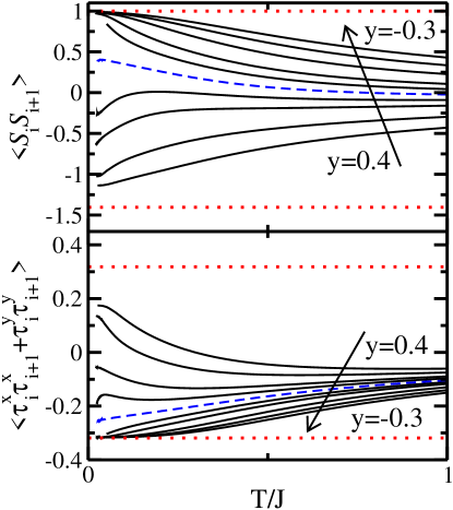
Figure 2: (Color online) Nearest-neighbor spin and orbital correlation functions for the spin-orbital model (7) with $\Gamma=1$ as a function of temperature $T$ in units of $J$ (we set $k_{\text{B}}=1$). In both panels $y=0.4$, 0.3, 0.2, 0.15, 0.1, 0.05, 0.0, $-0.1$, $-0.2$, $-0.3$ in arrow direction. The spin correlations switch from AF to FM at $y=0.1$ (dashed lines). The dotted lines in the upper (lower) panel correspond to the limiting values $1$ and $-1.4015$ ($-1/\pi$ and $1/\pi$), respectively.

In Fig. 2 the nearest-neigbor spin and orbital correlation functions for $\Gamma=1$ as a function of temperature for various parameters $y$ obtained by TMRG are shown. This method allows us to obtain thermodynamic quantities for 1D quantum systems directly in the thermodynamic limit.Bursill et al. (1996); Wang and Xiang (1997); Sirker and Klümper (2002) For $y\lesssim 0.1$ the ground state has ferromagnetically aligned spins. The phase transition between the fully polarized FM state and a state with AF spin correlations at $y\approx 0.1$ is first order. In the limit $y\gg 1$ the value $\langle\boldsymbol{S}_{j}\boldsymbol{S}_{j+1}\rangle\simeq-1.4015$ for a Haldane $S=1$ Heisenberg chain is reached,White and Huse (1993) while the orbital correlations approach $\langle\tau^{x}_{j}\tau^{x}_{j+1}+\tau^{y}_{j}\tau^{y}_{j+1}\rangle\to 1/\pi$. We note that the FM ground state is lost at $y\simeq 0.1$ both in the model with $\Gamma=1$ investigated here as well as in the model with an isotropic pseudospin sector ($\Gamma=0$).Miyashita and Kawakami (2005); Sirker and Khaliullin (2003) For the model with $\Gamma=1$, however, we have a direct phase transition from the FM to the Haldane phase while for the isotropic model an orbital valence bond phase is intervening between these two phases.Miyashita and Kawakami (2005)

The isotropic model (7), $\Gamma=0$, has also been intensely studied for $S=\tau=1/2$. Here the phase diagram is more complex than in the $S=1$, $\tau=1/2$ case.Itoi et al. (2000b); Chen et al. (2007) For $x=1$ the FM spin state is again found to be stable for $y\lesssim 0.1$. However, now the transition at $y\sim 0.1$ is to a gapless “renormalized $\text{SU}(4)$” phase followed by a further phase transition at larger $y$ into a dimer phase. The phase with ferromagnetically polarized orbitals is absent because $\langle\boldsymbol{S}_{j}\cdot\boldsymbol{S}_{j+1}+x\rangle>0$ for $x=1$ but is again present for large $y$ if $x\lesssim\ln 2-1/4$.

II.2 Boson-fermion model

For the 1D spin-orbital model, Eq. (7), at the point $\Gamma=1$, we will now derive an effective BF model which will be used as a starting point for the perturbative approach. First, applying the Jordan-Wigner transformation the orbital part is mapped onto a free fermion model (for $\Gamma\neq 1$ the pseudospins map onto interacting fermions). The spin part of the spin-orbital Hamiltonian (7) will be represented by bosons. Concentrating on the case where the spin part is ferromagnetically polarized in the ground state, we can treat the spin sector by the MSWT.Takahashi (1987, 1986) To this end, we introduce bosonic operators by a Dyson-Maleev transformation. If we retain bosonic operators only up to quadratic order we end up with

$$H\equiv\mathcal{H}_{S\tau}(1)-JN(S^{2}+x)y\simeq H_{0}+H_{1}\,.$$ (9)

Here $H_{0}$ is already diagonal

$$H_{0}=\sum_{k}\omega_{\text{B}}(k)b_{k}^{\dagger}b_{k}^{\ }+\sum_{q}\omega_{\text{F}}(q)f_{q}^{\dagger}f_{q}^{\ }\,,$$ (10)

with $f_{q}^{\dagger}$ and $f_{q}^{\ }$ ($b_{k}^{\dagger}$ and $b_{k}$) being the fermionic (bosonic) creation and annihilation operators, respectively. The magnon dispersion is given by

$$\omega_{\text{B}}(k)=2JS|y|(1-\cos k)\,,$$ (11)

and the fermion dispersion reads

$$\omega_{\text{F}}(q)=J(S^{2}+x)\cos q\,.$$ (12)

The spinless fermions fill up the Fermi sea between the Fermi points at $k_{F}=\pm\pi/2$.

For FM spin chains usual spin-wave theory has to be modified by a Lagrange multiplier $\mu$ acting as a chemical potential which enforces the Mermin-Wagner theorem of vanishing magnetization at finite temperatureTakahashi (1987)

$$S=\frac{1}{N}\sum_{k}\left<b_{k}^{\dagger}b_{k}^{\ }\right>.$$ (13)

Thermodynamic quantities calculated with this method are in excellent agreement with the exact Bethe ansatz solution for the uniform chain as well as with numerical TMRG data for the dimerized FM chain for temperatures up to $T\sim|J_{\text{eff}}|S^{2}$, with $J_{\text{eff}}$ being the effective exchange constant of the model under consideration.Sirker et al. (2008); Takahashi (1987, 1986); Herzog et al. (2010)

The interacting part couples bosons and fermions and reads

$$H_{1}=\frac{1}{N}\sum_{k_{1},k_{2},q}\omega_{\text{BF}}(k_{1},k_{2},q)b_{k_{1}}^{\dagger}b_{k_{2}}^{\ }f_{q}^{\dagger}f_{k_{1}-k_{2}+q}^{\ },$$ (14)

with the vertex

$$\omega_{\text{BF}}(k_{1},k_{2},q)\equiv JS\left[\cos(k_{2}-q)+\cos(k_{1}+q)\right.$$ (15)

$$\left.-\cos(k_{1}-k_{2}+q)-\cos q\right].$$

The Hamiltonian $H=H_{0}+H_{1}$ with $H_{0}$ and $H_{1}$ given by Eqs. (10) and (14), supplemented by the constraint (13), is an effective BF representation valid at low temperatures. We will investigate this model in Sec. V treating the BF coupling perturbatively.

III Mean-field decoupling

The spin-orbital model (7) contains rich and interesting physics. A first attempt to understand the properties of the model is to apply a MF decoupling which neglects the coupled spin-orbital degrees of freedom and treats the spin-orbital chain as two separate chains with effective coupling constants which have to be determined self-consistently. Note, however, that this treatment does not involve site variables as in the classical Weiss-MF theory but takes the correlations on a bond as relevant variables. Interestingly, these expectation values never vanish, which makes them useful particularly in cases without long-range order.

III.1 Decoupling into spin and orbital chain

Applying a MF decoupling and allowing for a dimerization in both sectorsSirker et al. (2008); Oleś et al. (2006) we obtain from Eq. (7)

$$\mathcal{H}_{S\tau}(\Gamma)\simeq H^{\text{MF}}_{S}+H^{\text{MF}}_{\tau}(\Gamma)\,,$$ (16)

with the spin and orbital Hamiltonians

$$H^{\text{MF}}_{S}=\mathcal{J}_{S}\sum_{j=1}^{N}\{1+(-1)^{j}\delta_{S}\}\boldsymbol{S}_{j}\cdot\boldsymbol{S}_{j+1}\,,$$ (17)

$$H^{\text{MF}}_{\tau}(\Gamma)=\mathcal{J}_{\tau}\sum_{j=1}^{N}\{1+(-1)^{j}\delta_{\tau}\}\left[\boldsymbol{\tau}_{j}\cdot\boldsymbol{\tau}_{j+1}\right]_{\Gamma}.$$

Within this approximation the effective superexchange constants and dimerization parameters are given by

$$\mathcal{J}_{\tau} =J\,\frac{\Delta^{+}_{SS}+2x}{2}, \qquad\delta_{\tau}=\frac{\Delta_{SS}^{-}}{\Delta_{SS}^{+}+2x}\,,$$ (18)

$$\mathcal{J}_{S} =J\,\frac{\Delta^{+}_{\tau\tau}+2y}{2}, \qquad\delta_{S}=\frac{\Delta_{\tau\tau}^{-}}{\Delta_{\tau\tau}^{+}+2y}\,,$$

where we have defined

$$\Delta_{SS}^{\pm} =\left<\boldsymbol{S}_{2j}\cdot\boldsymbol{S}_{2j+1}\right>\pm\left<\boldsymbol{S}_{2j}\cdot\boldsymbol{S}_{2j-1}\right>,$$ (19)

$$\Delta_{\tau\tau}^{\pm} =\left<\left[\boldsymbol{\tau}_{2j}\cdot\boldsymbol{\tau}_{2j+1}\right]_{\Gamma}\right>\pm\left<\left[\boldsymbol{\tau}_{2j}\cdot\boldsymbol{\tau}_{2j-1}\right]_{\Gamma}\right>.$$

Here $\Delta_{\sigma\sigma}^{-}$ with $\sigma=S$ ($\sigma=\tau$) is an order parameter for the spin (orbital) dimerization, respectively. Thus, the exchange constants and dimerization parameters for each sector are determined by the nearest-neighbor correlation functions in the other sector, making a self-consistent calculation necessary. In the following we want to solve Eqs. (17)-(19) for the spin exchange being effectively FM, i.e. $\mathcal{J}_{S}<0$.

III.2 Dimerized orbital correlations

Numerical investigations of the model with isotropic orbital exchange, $\mathcal{H}_{S\tau}(0)$, have shown orbital-singlet formation in the ground stateMiyashita and Kawakami (2005) for $y\gtrsim 0.1$. Moreover, although the ground state consists of a fully spin polarized FM state for $y\lesssim 0.1$ with AF orbital correlations, it has been shown that a tendency towards orbital singlet formation is still present but has to be activated by thermal fluctuations.Sirker and Khaliullin (2003) In Ref. Sirker et al., 2008 the model (16) was studied in the FM regime with $x=1$, $y=\frac{1}{4}-\gamma_{\textnormal{H}}$, $\Gamma=0$ and $\gamma_{\textnormal{H}}=0.1$ in order to address the question whether this orbital-Peierls effect can be captured within a MF decoupling approach. A dimerized phase for $0.10\lesssim T/J\lesssim 0.49$ (we set $k_{\text{B}}=\hbar=1$) was found with the dimerization amplitude in the spin sector being much larger than in the orbital sector.

We now want to compare this result with the case where we set $\Gamma=1$ in Eq. (16) so that the self-consistent Eqs. (18) can be solved analytically by applying a Jordan-Wigner transformation and MSWT. Introducing fermionic operators $f^{(\dagger)}_{j,e}$ if the index $j$ is even and $f^{(\dagger)}_{j,o}$ if $j$ is odd for the pseudospins, we rewrite $H^{\text{MF}}_{\tau}\equiv H^{\text{MF}}_{\tau}(\Gamma=1)$ in Fourier representation. Finally introducing new fermionic operators $\phi^{(\dagger)}_{q}$ and $\varphi^{(\dagger)}_{q}$ which diagonalize the Hamiltonian $H^{\text{MF}}_{\tau}$, we find

$$H^{\text{MF}}_{\tau}=\sum_{q}\omega^{\text{MF}}_{\text{F}}(q,\delta_{\tau})(\phi_{q}^{\dagger}\phi_{q}^{\ }+\varphi_{q}^{\dagger}\varphi_{q}^{\ })\,,$$ (20)

with the fermionic dispersionPincus (1971)

$$\omega^{\text{MF}}_{\text{F}}(q,\delta_{\tau})\equiv\mathcal{J}_{\tau}\sqrt{\cos^{2}q+\delta_{\tau}^{2}\sin^{2}q}\,.$$ (21)

We can now calculate $\Delta_{\tau\tau}^{\pm}$, as given in Eq. (19) straightforwardly and obtain

$$\Delta_{\tau\tau}^{-} = \!\!\!\frac{2\delta_{\tau}}{N}\sum_{q}\frac{\left\{2n_{\textnormal{F}}[\omega^{\text{MF}}_{\text{F}}(q,\delta_{\tau})]-1\right\}\sin^{2}q}{\sqrt{\cos^{2}q+\delta_{\tau}^{2}\sin^{2}q}},$$ (22)

$$\Delta_{\tau\tau}^{+} = \!\!\!\frac{2}{N}\sum_{q}\frac{\left\{2n_{\textnormal{F}}[\omega^{\text{MF}}_{\text{F}}(q,\delta_{\tau})]-1\right\}\cos^{2}q}{\sqrt{\cos^{2}q+\delta_{\tau}^{2}\sin^{2}q}},$$

where $n_{\textnormal{F}}(x)=\left\{\exp(\beta x)+1\right\}^{-1}$ is the Fermi function and $\beta=1/T$.

III.3 Dimerized spin correlations

Next we turn to the spin part of Eq. (16) to which we apply the MSWT.Takahashi (1987, 1986) We introduce two bosonic operators $b^{(\dagger)}_{j,e}$ [$b^{(\dagger)}_{j,o}$] for $j$ even [odd] by means of a Dyson-Maleev transformation. Retaining only terms bilinear in the bosonic operators we can diagonalize the resulting Hamiltonian by a Bogoliubov transformation leading to

$$H^{\text{MF}}_{S}= \sum_{k}\left\{\omega^{\text{MF}}_{\text{B},-}(k,\delta_{S})\alpha_{k}^{\dagger}\alpha_{k}^{\ }+\omega^{\text{MF}}_{\text{B},+}(k,\delta_{S})\beta_{k}^{\dagger}\beta_{k}^{\ }\right\}$$ (23)

$$+\mathcal{J}_{S}NS^{2}\,,$$

with the two magnon branches

$$\omega_{\text{B},\pm}^{\text{MF}}(k,\delta_{S})=2|\mathcal{J}_{S}|S\left(1\pm\sqrt{\cos^{2}k+\delta_{S}^{2}\sin^{2}k}\right)\,.$$ (24)

The constraint of vanishing magnetization at finite temperature (13) now reads

$$S=\frac{1}{N}\sum_{k}\left\{n_{\textnormal{B}}[\zeta^{-}(k,\delta_{S})]+n_{\textnormal{B}}[\zeta^{+}(k,\delta_{S})]\right\},$$ (25)

where $n_{\textnormal{B}}(x)=\{\exp\{\beta x\}-1\}^{-1}$ is the Bose function and $\zeta^{\pm}(k,\delta_{S})=\omega^{\text{MF}}_{\textnormal{B},\pm}(k,\delta_{S})-\mu(\delta_{S})$.

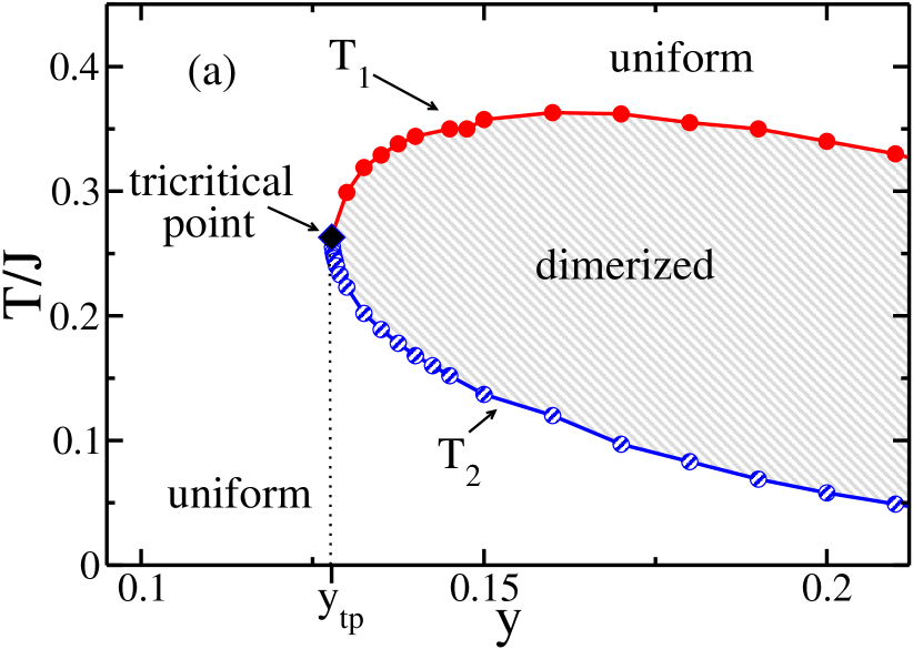
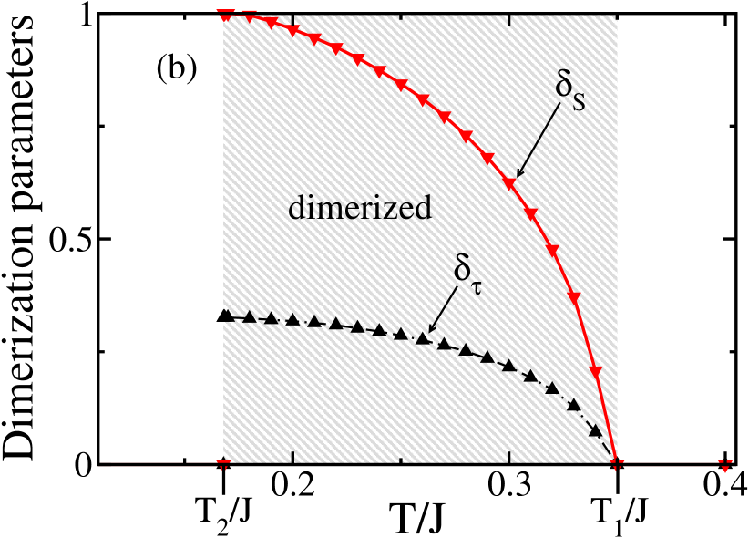
Figure 3: (a) Phase diagram of the Hamiltonian (16) with $\Gamma=1$ and $x=1$ in mean-field decoupling. The shaded area represents the dimerized phase. The phase transition at $T_{2}$ is first order whereas the transition at $T_{1}$ is of second order. The two transition lines merge at the tricritical point $y_{\text{tp}}$. (b) Dimerization parameters $\delta_{S}$ and $\delta_{\tau}$ for $x=1$ and $y=0.14$. The lines are guides to the eye. The shaded area marks the temperature range where the dimerization is nonzero.

To calculate the nearest-neighbor correlation functions $B_{\pm}\equiv\bigl{<}\boldsymbol{S}_{j}\cdot\boldsymbol{S}_{j\pm 1}\bigr{>}$ it is necessary to go beyond linear spin-wave theory. Taking terms of quartic order into account and using Eq. (25) we obtainSirker et al. (2008)

$$B_{\pm}=\left(\frac{1}{N}\sum_{k}f_{\pm}(k,\delta_{S})\sum_{\sigma\in\{\pm\}}\sigma n_{\textnormal{B}}[\zeta^{\sigma}_{B}(k,\delta_{S})]\right)^{2}.$$ (26)

Here we have defined

$$f_{\pm}(k,\delta_{S})\equiv\frac{\cos^{2}k\pm\delta_{S}\sin^{2}k}{\sqrt{\cos^{2}k+\delta_{S}^{2}\sin^{2}k}}\,.$$ (27)

From these expressions we can obtain $\Delta_{SS}^{\pm}$ which, combined with Eq. (22), allows us to solve Eqs. (16)-(19) self-consistently.

III.4 Mean-field phase diagram

We first discuss the ground state phase diagram of the Hamiltonian (16) for $\Gamma=1$. Depending on the sign of the effective coupling constant $\mathcal{J}_{S}$ we find $\langle\boldsymbol{S}_{j}\boldsymbol{S}_{j+1}\rangle=1,\,-1.4015$ with the latter value being the approximate result for the $S=1$ AF Haldane chain. In the following, we restrict our discussion to $-1<x<1.4015$ so that $\langle\boldsymbol{S}_{j}\boldsymbol{S}_{j+1}\rangle$ and $\mathcal{J}_{\tau}=J(\langle\boldsymbol{S}_{j}\boldsymbol{S}_{j+1}\rangle+x)$ always have the same sign. For the orbital sector we obtain, on the other hand, $\langle\tau^{x}_{j}\tau^{x}_{j+1}+\tau^{y}_{j}\tau^{y}_{j+1}\rangle=\pm 1/\pi$. $y>1/\pi$ implies $\mathcal{J}_{S}>0$ and the ground state is therefore certainly AF (Haldane phase) whereas $\mathcal{J}_{S}<0$ for $y<-1/\pi$ leading to a FM state. In the regime $-1/\pi<y<1/\pi$ the self-consistent equations have two solutions with energies $E_{0}^{\text{AF}}\approx(1/\pi+y)(-1.4015+x)$ and $E_{0}^{\text{FM}}=(-1/\pi+y)(1+x)$ and a first order phase transition between the FM and AF states occurs where the energies cross. For the case $x=1$ we are focussing on here, this happens at $y_{c}\approx 0.212$ and the FM state is stable for $y<y_{c}$. Compared to the numerical solution where $y_{c}\approx 0.1$ (see Fig. 2) the range of stability of the FM state is therefore increased in the MF solution.

Next, we investigate the possibility of a finite temperature dimerization for $x=1$ in that part of the phase diagram where the ground state is FM. As shown in Fig. 3(a) we find that a dimerized phase at finite temperatures does indeed exist in MF decoupling for $y_{\text{tp}}\approx 0.128\lesssim y\lesssim y_{c}\approx 0.212$ where $y_{\text{tp}}$ denotes the tricrictal point. As in the model with an isotropic pseudospin sector,Sirker et al. (2008) the temperature range where the dimerized phase is stable depends on $y$. At the onset temperature $T_{1}$ the phase transition is of second order whereas at the reentrance temperature $T_{2}$ it is of first order, see Fig. 3(b). As in the case $\Gamma=0$, the dimerization in the spin sector is always much larger than in the orbital sector.

As pointed out before, the MF decoupling suffers from severe limitations and it is expected to be an even worse approximation in the extreme quantum case $\Gamma=1$ than in the case $\Gamma=0$ studied previously.Sirker et al. (2008) In particular the coupling between spin and orbital degrees of freedom is completely lost within this approach. In the following sections we will therefore develop an alternative perturbative treatment of the spin-orbital coupling.

IV Dynamical spin structure factor for the uniform ferromagnetic chain

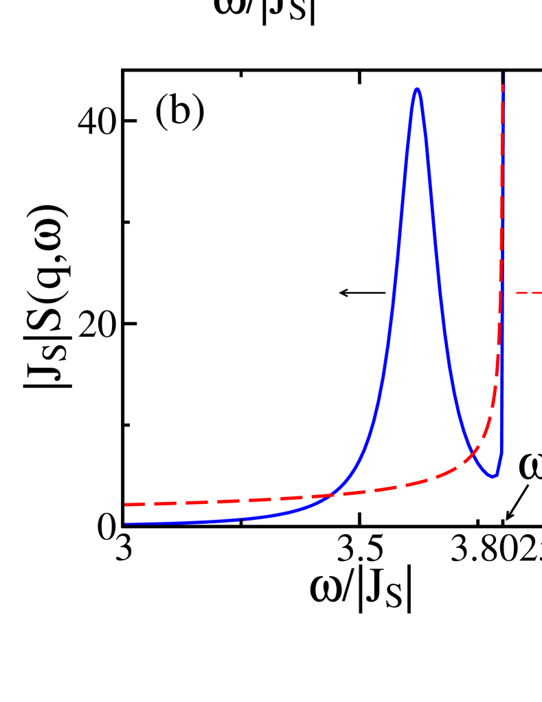
Figure 4: (Color online) (a) Dynamical spin structure factor $S(q,\omega)$ as obtained for $T/|J_{S}|=0.1$ and $0\leq q\leq\pi$. The dashed line indicates the upper boundary of the two magnon continuum. The dots are projections of the peak positions onto the $(q,\omega)$ plane. They are connected by the dotted line which is a guide to the eye. (b) Dynamical spin structure factor $S(q,\omega)$ for the same parameters at $q=4\pi/5$ (solid line) and the corresponding density of states (dashed line).

In order to investigate coupled spin-orbital degrees of freedom and, in particular, their implications on the spin dynamics of the spin-orbital chain, a detailed understanding of the spin dynamics of a FM chain is useful. We shall avoid the complications of the dimerized chain and focus our study on the uniform 1D ferromagnet.rem (b) In doing so we neglect the coupling between spin and pseudospin operators for a moment and consider

$$H_{S}=J_{S}\sum_{j}\boldsymbol{S}_{j}\cdot\boldsymbol{S}_{j+1}\,,$$ (28)

with $J_{S}<0$. It is well-known that MSWT does not respect the SU(2) symmetry of the FM Heisenberg chain Eq. (28). We therefore directly calculate the full spin correlation functionTakahashi (1990, 1993)

$$G(r,\tau)\equiv-\left<\mathcal{T}[\textbf{S}_{j}(0)\cdot\textbf{S}_{j+r}(\tau)]\right>\;.$$ (29)

In Fourier space we obtain

$$G(q,\omega_{\nu,\textnormal{B}})\!=\frac{1}{N}\sum_{k}(1+n_{\textnormal{B}}[\zeta(k)])n_{\textnormal{B}}[\zeta(q-k)]\frac{1-\textnormal{e}^{-\beta\epsilon_{q}(k)}}{i\omega_{\nu,\textnormal{B}}-\epsilon_{q}(k)},$$ (30)

where we have used the bosonic Matsubara frequencies $\omega_{\nu,\textnormal{B}}$ and $\epsilon_{q}(k)\equiv\zeta(k)-\zeta(q-k)$ with $k\in[-\pi,\pi]$. The reduced magnon dispersion reads

$$\zeta(k)=2J_{S}S(1-\cos k)-\mu.$$ (31)

In Fig. 4(a) the dynamical spin structure factor,

$$S(q,\omega)=2n_{\text{B}}(-\omega)\,\textnormal{Im}G^{\textnormal{ret}}(q,\omega),$$ (32)

is shown for the uniform FM chain at $\omega>0$, where

$$\textnormal{Im}G^{\textnormal{ret}}(q,\omega)= \frac{\pi}{N}\sum_{k}(1+n_{\textnormal{B}}[\zeta(k)])n_{\textnormal{B}}[\zeta(q-k)]$$ (33)

$$\times\left(\textnormal{e}^{-\beta\epsilon_{q}(k)}-1\right)\delta(\omega-\epsilon_{q}(k))$$

is the imaginary part of the retarded Green’s function obtained from Eq. (30) by analytical continuation. Up to a factor of $2\pi$, as a matter of definition, we obtain the result previously given by Takahashi.Takahashi (1990) The structure factor fulfills detailed balance, $S(q,\omega)=\textnormal{e}^{\beta\omega}S(q,-\omega)$. The symbols in Fig. 4 show the peak positions projected onto the $(q,\omega)$ plane. They follow the reduced dispersion Eq. (31). Also shown in Fig. 4(a) as a dashed curve is $\omega_{q}^{\textnormal{max}}=4|J_{S}|S\sin\frac{q}{2}$ corresponding to the upper boundary of the two magnon continuum $\epsilon_{q}(k)$ above which $S(q,\omega)$ is zero in this approximation.

At the edge of the two magnon continuum $S(q,\omega)$ has a singularity. In Fig. 4(b) the dynamical spin structure factor for the same parameters as used in Fig. 4(a) is shown at $q=4\pi/5$ together with the density of states which is given by $\rho_{q}(\omega)=1/\sqrt{(\omega_{q}^{\textnormal{max}})^{2}-\omega^{2}}$. Right below the singularity at $\omega_{q}^{\textnormal{max}}$ the density of states to lowest order reads $\rho_{q}(\omega_{q}^{\textnormal{max}}-\delta\omega)\sim 1/\sqrt{\delta\omega}$, i.e., $S(q,\omega)$ shows a square root divergence at the upper threshold. If the edge singularity and the central peak are well separated then the spectral weight of the edge singularity is much smaller than the spectral weight of the central peak. If, on the other hand, the edge singularity is close to the central peak then the shape of the latter is strongly affected by the occurence of the edge singularity. In this case the edge singularity gives a significant contribution.

It is instructive to analyze $S(q,\omega)$ in the limit of small $q$. If the edge singularity and the peak of the structure factor are well separated, the lineshape of the peak can be obtained approximately. To this end, for small $q$ but $|J_{S}|S^{2}q/T\gg 1$ we only retain the leading terms of Eq. (30). Performing a saddle point approximation to lowest order we find $S(q,\omega)\sim n_{\text{B}}(-\omega)(a(q,\omega)-a(q,-\omega))$, with

$$a(q,\omega)\approx 2S\frac{\frac{|J_{S}|Sq}{\xi}}{(\omega-J_{S}Sq^{2})^{2}+\left(\frac{J_{S}Sq}{\xi}\right)^{2}}\,.$$ (34)

This Lorentzian lineshape is only valid for low temperatures. Here $\xi\approx|J_{S}|S^{2}/T$ is the correlation length in the low-temperature limit.Takahashi (1987, 1986, 1990, 1993) Finally, we want to stress that for $T\to 0$ the peaks will reduce to $\delta$-functions, i.e., only thermal broadening is included in this approximation.

V Perturbation theory

In this section we intent to go beyond the MF decoupling approach treating the influence of the BF interaction, Eq (14), on the spin-wave dispersion perturbatively. Naively one would expect that the magnon should be able to couple to the fermionic degrees of freedom if it lies inside the fermionic two-particle continuum. The upper and lower boundary of the latter are given by

$$\epsilon_{\text{F}}^{\text{max}}(q) = 2J(S^{2}+x)\sin(q/2),$$

$$\epsilon_{\text{F}}^{\text{min}}(q) = J(S^{2}+x)\sin q,$$ (35)

respectively. The continuum and the magnon dispersion $\omega_{\text{B}}(q)$ for $y=-1$ are shown in Fig. 5. One would therefore expect that in this case $\omega_{\text{B}}(q)$ is unaffected by the presence of the fermions for $q<\pi/2$, since it can not couple to these degrees of freedom. However for higher momenta the spin wave may couple to the fermionic degrees of freedom and thus a broadening of $S(q,\omega)$ should occur. Moreover by choosing different values for $y$ the point at which the magnon enters the fermionic two-particle continuum is changed. Thus the momentum at which the spin wave is affected by the coupling to the fermionic degrees of freedom depends directly on the parameter $y$.

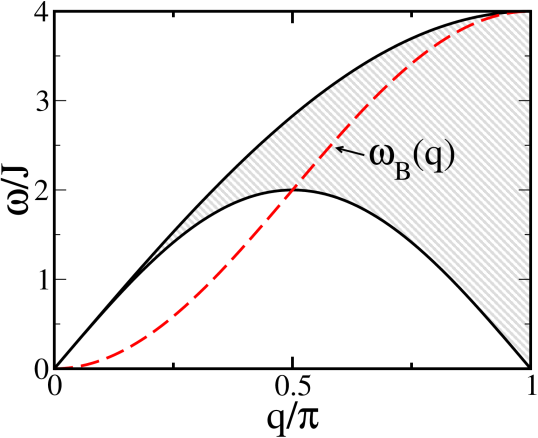
Figure 5: (Color online) Magnon dispersion $\omega_{\text{B}}(q)$ (dashed line) for $y=1$ and fermionic two-particle continuum (shaded area).

Figure 6: Diagrams which contribute to a renormalization of the magnon in a perturbation theory: (a,b) Diagrams with momentum exchange between the magnon and the fermions, and (c) diagram without momentum exchange. All diagrams are second order. Fermionic propagators are shown by solid lines, whereas bosonic propagators are shown as dashed lines.

These arguments give the qualitatively correct picture, i.e., we find indeed that the coupling of the magnon to the fermionic degrees of freedom has strong effects on the dynamical spin structure factor at intermediate and high momenta and that the onset of these effects can be well estimated by our simple argument. However, there are also certain aspects which can not be captured within this picture. For instance, for $2S|y|>(S^{2}+x)$ it suggests that the spin wave may leave the fermionic two-particle continuum at a certain momentum $q_{l}$ and thus should be unaffected by the BF coupling for $q>q_{l}$. The detailed calculation, however, reveals that this is not true because the spin wave decays into a fermionic particle-hole and a remaining spin wave as will become clear in the following.

V.1 General formulation

Here we want to study the Hamiltonian $H$ given by Eq. (9), with its noninteracting part $H_{0}$ and interacting part $H_{1}$ defined by Eqs. (10) and (14), by treating the BF interaction perturbatively, i.e., in the limit $|x|,|y|\gg 1$. As explained in the appendix, we start by performing a MF decoupling for the interaction $H_{1}$. Corrections to this solution are then taken into account perturbatively. Here we adress the bosonic Green’s function at zero temperature

$$\mathcal{G}_{\textnormal{B}}^{\ }(q,t)=-i\left<\mathcal{T}_{t}\left[b_{q}^{\ }(t)b_{q}^{\dagger}(0)\right]\right>.$$ (36)

In Fig. 6 all distinct, connected diagrams beyond the MF decoupling up to second order are shown.

We calculate the Green’s function from the Dyson equation

$$\mathcal{G}_{\text{B}}(q,\omega)=\frac{1}{\left\{\mathcal{G}_{\text{B}}^{(0)}(q,\omega)\right\}^{-1}-\Sigma(q,\omega)},$$ (37)

with

$$\left\{\mathcal{G}^{(0)}_{\text{B}}(q,\omega)\right\}^{-1}=\omega-\zeta(q),$$ (38)

where $\zeta(q)$ is the reduced magnon dispersion defined in Eq. (31) with $J_{S}=J(y-1/\pi)$, and the self-energy $\Sigma(q,\omega)$ is approximated by the proper self-energy $\Sigma_{2}(q,\omega)$ obtained by summing up the diagrams which can be composed of the diagrams shown in Fig. 6.

Figure 7: Second order diagram for a system of interacting fermions with momentum exchange.

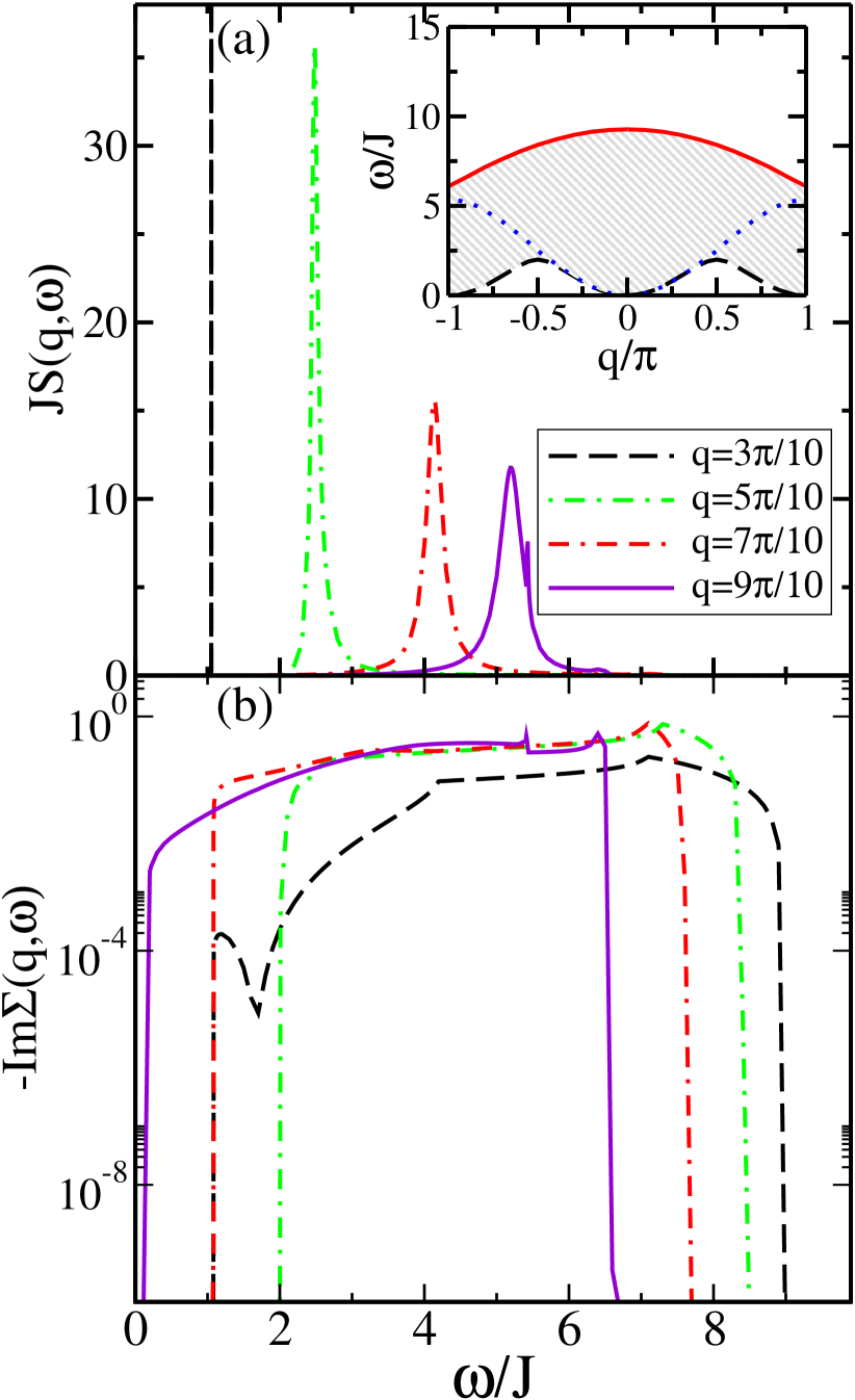
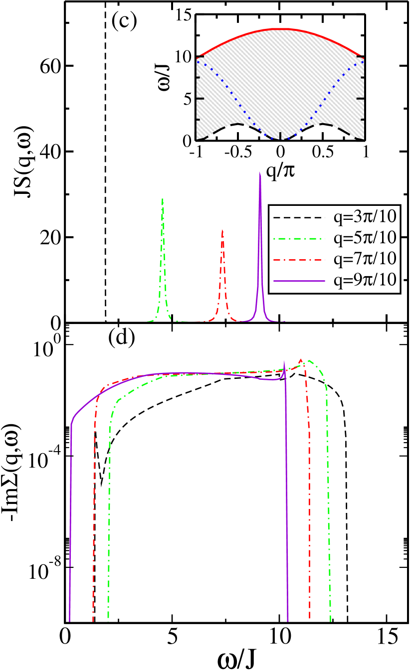
Figure 8: (Color online) Perturbative results for the BF model at zero temperature with $x=1$. In the left (right) panel $y=-1$ ($y=-2$), respectively. (a),(c) $S(q,\omega)$ with the inset showing the region for which $\text{Im}\,\Sigma_{\text{BF}}^{+}(q,\omega)$ is nonzero as a shaded area and the renormalized spin-wave dispersion as a dotted line. While $S(q,\omega)$ is sharply peaked at low momenta, a significant broadening occurs at higher $q$. Moreover we find additional structures which, as explained in the text, are due to coupled spin-orbital excitations. (b),(d) $-\text{Im}\,\Sigma_{\text{BF}}^{+}(q,\omega)$ as given in Eq. (39) for the corresponding values of $q$ shown in (a) and (c), respectively. The coupled spin-orbital excitations show up as peaks and edges in $\text{Im}\,\Sigma_{\text{BF}}^{+}(q,\omega)$ (notice the logarithmic scale).

The diagrams shown in Figs. 6(a) and 6(b) are of particular interest because they are the lowest order diagrams where bosons and fermions exchange momentum. They describe the part of spin-orbital dynamics which cannot be captured within the MF decoupling approach discussed in section III. The diagram shown in Fig. 6(b) has to be thermally activated, i.e., it does not give any contribution at zero temperature. The same is true for the diagram shown in Fig. 6(c). Thus at $T=0$ the only second order diagram which contributes to the self energy is the one shown in Fig. 6(a) leading to

$$\Sigma_{\text{BF}}^{+}(q,\omega)= -\frac{1}{N^{2}}\sum_{k_{1},k_{2}}\omega^{2}_{\text{BF}}(q,k_{1},k_{2})$$ (39)

$$\times\frac{\Theta[\omega_{\text{F}}(q-k_{1}+k_{2})]\Theta[-\omega_{\text{F}}(k_{2})]}{\omega-\Omega^{+}_{q}(k_{1},k_{2})+i0^{+}}\,,$$

where we have abbreviatedFT

$$\Omega^{\pm}_{q}(k_{1},k_{2})\equiv\pm\zeta(k_{1})+\omega_{\text{F}}(q-k_{1}+k_{2})-\omega_{\text{F}}(k_{2})\,,$$ (40)

with $k_{1},k_{2}\in[-\pi,\pi]$.

For systems of interacting fermions we know that perturbation theory in one dimension often leads to infrared divergencies.Giamarchi (2003); Metzner et al. (1998) Such divergencies occur, for example, for the fermionic analogon of the diagram with momentum exchange, see Fig. 7. These problems can be overcome by the Dzyaloshinski-Larkin solution or bosonization techniques. For the model considered here, however, we find no divergencies within the considered diagrams. One reason for this behavior is a lack of nesting. While for a fermionic interaction as shown in Fig. 7 all the dispersions in the denominator of Eq. (39) are approximately linear at low energies here one of the dispersions is approximately quadratic so that nesting only occurs for singular points. As a further check, we have evaluated the integrals in Eq. (39) for a constant vertex at small $q$ and $\omega$ and did not find any infrared divergencies.

For finite temperatures the Matsubara formalism can be applied straightforwardly. The self-energy Eq. (39) now reads

$$\Sigma_{\text{BF}}^{+}(q,\omega_{\nu,\textnormal{B}}) = -\frac{1}{N^{2}}\sum_{k_{1},k_{2}}\frac{\omega^{2}_{\text{BF}}(q,k_{1},k_{2})}{i\omega_{\nu,\textnormal{B}}-\Omega^{+}_{q}(k_{1},k_{2})}$$

$$\!\!\!\!\!\!\!\!\!\!\!\!\!\!\!\!\times \!\!\!\!\!\!\!\!\!\!\!\!\mathcal{N}^{+}_{\textnormal{F,B}}(k_{1},k_{2},\omega_{\nu,\textnormal{B}},T)\mathcal{N}_{\textnormal{F,F}}(q,k_{1},k_{2},\omega_{\nu,\textnormal{B}},T),$$

where we have abbreviated

$$\mathcal{N}^{\pm}_{\textnormal{F,B}}(k_{1},k_{2},\omega_{\nu,\textnormal{B}},T)\!\! \equiv \!\!n_{\textnormal{B}}[\zeta(k_{1})]\pm n_{\textnormal{F}}[\omega_{\text{F}}(k_{2})],$$

$$\!\!\!\mathcal{N}_{\textnormal{F,F}}(q,k_{1},k_{2},\omega_{\nu,\textnormal{B}},T)\!\! \equiv \!\!n_{\textnormal{F}}[\omega_{\text{F}}(q-k_{1}+k_{2})]$$ (42)

$$-n_{\textnormal{F}}[\omega_{\text{F}}(k_{2})-\zeta(k_{1})].$$

Note that at finite temperatures both, the reduced spin-wave dispersion $\zeta(q)$ as well as the fermionic dispersion is renormalized due to the MF decoupling applied to Eqs. (14). The respective expressions are given in the appendix, see Eqs. (54) and (55).

At finite temperatures also the diagram shown in Fig. 6(b) contributes and is given by

$$\Sigma_{\text{BF}}^{-}(q,\omega_{\nu,\text{B}})=-\frac{1}{N^{2}}\sum_{k_{1},k_{2}}\frac{\omega_{\text{BF}}^{2}(q,k_{1},k_{2})}{i\omega_{\nu,\text{B}}-\Omega^{-}_{q}(k_{1},k_{2})}$$ (43)

$$\times(1+\mathcal{N}^{-}_{\textnormal{F,B}}(k_{1},k_{2},\omega_{\nu,\textnormal{B}},T))\mathcal{N}_{\textnormal{F,F}}(q,k_{1},k_{2},\omega_{\nu,\textnormal{B}},T).$$

V.2 Dynamical spin structure factor

Below we present the results obtained by summing up the diagrams shown in Fig. 6 in a Dyson series, but replacing the external legs by the SU(2) symmetric function given in Eq. (30). While the perturbative results can, strictly speaking, only be valid for $|x|,|y|\gg 1$ we extend the results here to more physical values $|x|,|y|\sim\mathcal{O}(1)$ where we still expect perturbation theory to give at least a qualitatively correct picture. Numerical results obtained for the dynamical spin structure factor within this perturbative approach are shown in Fig. 8 for $T=0$ and $y=-1$ and $y=-2$. In both cases $S(q,\omega)$ is sharply peaked at small momenta whereas a significant broadening occurs at higher momenta. Note, that within the MSWT $S(q,\omega)$ is always a $\delta$-function for the pure spin model at $T=0$, i.e., the broadening here is solely due to the coupling to orbital excitations.

By extracting the central peaks of the dynamical spin structure factor at various momenta, we obtain the renormalized spin-wave dispersion $\omega_{q}$ within the perturbative approach. The result of this is shown in the insets of Fig. 8(a,c) and in more detail in Fig. 9. The magnon dispersion is renormalized and small kinks are visible close to $q=\pi/2$, which may be interpreted as Kohn anomalies (see below). The inset of Fig. 9 shows the Kohn anomalies with a higher resolution. For itinerant ferromagnets Kohn anomalies are well-known. Here the interaction between the spins of localized ions is mediated by an exchange with the conduction electrons.Kohn (1959); Woll and Nettel (1961); Barnea and Horwitz (1975); Møller and Houmann (1966); Halilov et al. (1998); Pajda et al. (2001); Morán et al. (2003) These Kohn anomalies can thus be used to gain information about the Fermi surface of the conduction electrons.Kohn (1959); Woll and Nettel (1961); Barnea and Horwitz (1975) However to the best of our knowledge Kohn anomalies in the spin-wave dispersion for insulating materials have not been adressed so far. As we will show below, the Kohn anomalies in our case are caused by coupled spin-orbital degrees of freedom.

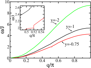
Figure 9: (Color online) Renormalized magnon dispersions $\omega_{q}$ in the FM chain for $x=1$ and selected values of $y$. Inset: The most pronounced Kohn anomalies occur at $q$ near $\pi/2$.

Apart from extracting the effective spin-wave dispersion from $S(q,\omega)$, we also want to discuss the magnon bandwidth (full width at half maximum (FWHM)) $\Gamma_{q}$ of the central peaks. A broadening of the zero temperature peaks occurs whenever the imaginary part of the self-energy,

$$\text{Im}\ \Sigma_{\text{BF}}^{+}(q,\omega) = -\frac{\pi}{N^{2}}\sum_{k_{1},k_{2}}\omega^{2}_{\text{BF}}(q,k_{1},k_{2})\Theta[-\omega_{\text{F}}(k_{2})]$$

$$\times \Theta[\omega_{\text{F}}(q-k_{1}+k_{2})]\delta(\omega-\Omega^{+}_{q}(k_{1},k_{2})),$$

is non-zero at $\omega=\Omega^{+}_{q}(k_{1},k_{2})$. The contributions within the sums are now determined by the argument of the $\delta$-function as well as by the constraints given by the Heaviside functions. This procedure, for a given set of parameters $x,y,$ and $S$, effectively yields a region within which the spin wave may scatter on fermion pairs. Henceforth we call this region the BF continuum. The BF continuum is shown in the insets of Figs. 8(a) and 8(c) as shaded areas. The upper boundary of the BF continuum (solid lines), which is periodic with a period of $2\pi$, is given by $-4JS(y-1/\pi)+2J(S^{2}+x)$ for $q=0$, and decreases monotonously from this value with increasing $|q|$. The lower boundary (dashed lines) is periodic with a period of $\pi$.

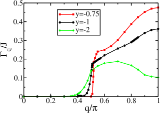
Figure 10: (Color online) Magnon linewidth $\Gamma_{q}$ (FWHM of $S(q,\omega)$) at zero temperature (data points), as obtained for $x=1$ and the representative values of $y$ indicated in the plot. The lines are guides to the eye.

To obtain the FWHM of the structure factor, the magnitude of the contributions to the sums given in Eq. (V.2) are essential. Here not only the $(k_{1},k_{2})$-region which contributes to the summation but also the magnitude of the vertex $\omega_{\text{BF}}$ is of importance. We observe that the vertex is small at small momenta but increases at intermediate and high momenta. This leads to a strong increase of the magnitude of the imaginary part of the self-energy as shown in panels (b) and (d) of Fig. 8. From the insets of Fig. 8 it becomes clear that the spin-wave dispersion enters the BF continuum depending on $y$. For higher values of $|y|$ the spin wave enters at lower momenta. However, since the vertex gives smaller contributions at smaller momenta, the broadening of the central peaks of the dynamical spin structure factor turns out to be smaller the smaller the momenta are at which the spin wave enters the BF continuum. This can be seen in Fig. 10 where the magnon linewidth $\Gamma_{q}$ is shown. The onset of a finite $\Gamma_{q}$ signals the entrance of the spin-wave dispersion into the BF continuum and depending on the momentum at which the entrance occurs the increase of $\Gamma_{q}$ is either smooth (entrance at low momentum) or steep (entrance at high momentum). In addition, we observe that $\Gamma_{q}$ has a maximum at the boundary of the Brillouin zone for stronger interactions ($y=-0.75$ and $y=-1$ in Fig. 10 respectively), whereas for smaller interactions we observe the maximum at smaller momenta followed by a decrease of the FWHM towards the zone boundary ($y=-2$ in Fig. 10).

Interestingly, the coupling to the orbital degrees of freedom does not only give rise to a featureless broadening of $S(q,\omega)$ but produces additional structures. These additional structures are most obvious in Fig. 8(a). From Fig. 8(b) it becomes clear that these structures are dominated by local extrema as well as edges in the imaginary part of the self-energy. Eq. (V.2) shows that such extrema can occur if $\Omega^{+}_{q}(k_{1},k_{2})$, Eq. (40), becomes stationary as a function of the momenta $k_{1},k_{2}$ as long as the Heaviside functions in Eq. (V.2) for these momenta are non-zero. The position of the local maxima in the imaginary part of the self-energy is therefore approximately given by the values $\Omega^{+}_{q}(k_{1},k_{2})$ at these stationary points. These values correspond to the energy of spin-orbital excitations into which the initial spin wave can decay, see Fig. 6(a) and which are stable against small redistributions of momenta.

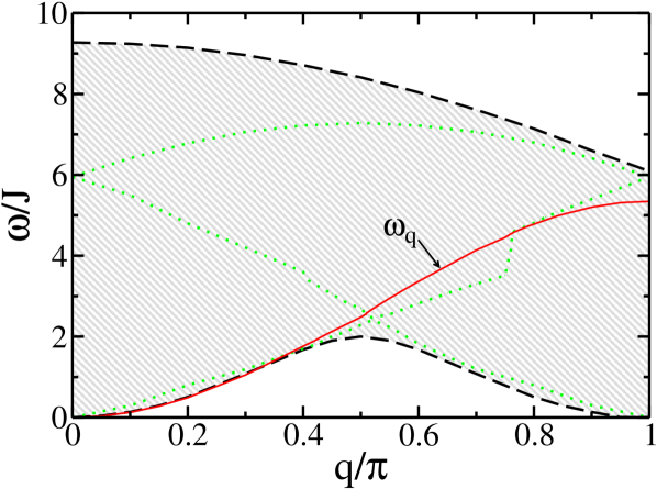
Figure 11: (Color online) Effective dispersion of the spin wave $\omega_{q}$ for $y=-1$ (red solid line) together with coupled spin-orbital excitations deduced from $-\text{Im}\,\Sigma_{2}(q,\omega)$, shown by (green) dots within the Bose-Fermi continuum (shadded area).

We conclude that while we do not have completely sharp spin-orbital excitations any more as in the Hamiltonian (6) with FM exchange considered in the introduction, there are still characteristic spin-orbital excitations of finite width within the spin-orbital continuum. As shown in Fig. 11 we can extract the dispersion of these characteristic excitations and find that the coupled spin-orbital excitations are gapless for the parameters considered here. However, as can be clearly seen in Figs. 8(b) and 8(d), the weights of the low-energy excitations are orders of magnitude smaller than the excitations located at higher energies. Hence the excitations at high energies give the most dominant contribution to the dynamical spin structure factor. We therefore expect that these excitations will generate additional entropy in the corresponding temperature range which should show up, for example, in the specific heat which will be studied in the next section.

Moreover, we find that these coupled spin-orbtial excitations are responsible for the Kohn anomalies mentioned above. We observe that the Kohn anomalies at intermediate momenta occur when the energy of the spin wave coincides with that of a characteristic spin-orbital excitation. This is different from the Kohn anomaly in the spin-wave dispersion of itinerant ferromagnets. In this case the interaction between the localized spins given by the lattice ions is induced by scattering with conduction electrons and hence the Kohn anomaly is determined by the shape of the Fermi surface.Kohn (1959); Woll and Nettel (1961); Barnea and Horwitz (1975); Møller and Houmann (1966); Halilov et al. (1998); Pajda et al. (2001); Morán et al. (2003) The Kohn anomaly we find within the present context is also due to interaction effects, where the nature of the interactions - coupled spin-orbital degrees of freedom - is distinct from the ones of the itinerant ferromagnets. For the case $x=-y=1$ the spin-wave dispersion has a discontinuity of the order $\Delta\omega\simeq 0.01J$ at the point $q\simeq 0.509\pi$ (see inset of Fig. 9). However, for the crossing points of the magnon and the coupled spin-orbital excitation located at $q\simeq 0.37\pi$ and $q\simeq 0.76\pi$ (see Fig. 11) no Kohn-anomaly could be resolved. We believe that this is a consequence of the weight of the coupled spin-orbital excitations: Whereas at $q\simeq 0.509\pi$ the imaginary part of the self-energy displays a steep increase of several magnitudes, at the other crossing points the slope towards the local maxima is far more moderate.

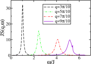
Figure 12: (Color online) Dynamical spin structure factor $S(q,\omega)$ calculated perturbatively for the spin-orbital chain at temperature $T/J=0.1$ with $y=-1$.

At finite temperatures two effects contribute to the broadening of the central peaks of the dynamical spin structure factor. First, there is a broadening due to thermally excited magnons which is already present in the 1D Heisenberg chain discussed in Sec. IV. This is combined with the broadening due to the interaction with the orbital degrees of freedom. Here the BF continuum is smeared out by thermal fluctuations compared to the zero temperature case. Results for the structure factor at finite temperatures are shown in Fig. 12.

The broadening at small momenta is dominated by thermal fluctuations and the lineshape is very similar to that of the pure spin model discussed in Sec. IV. A further strong broadening in going from $q=0.3\pi$ to $q=0.5\pi$ signals the relevance of coupled spin-orbital degrees of freedom on the spin dynamics at intermediate and high momenta. Again, additional structures in $S(q,\omega)$ are visible related to the spin-orbital excitations discussed above.

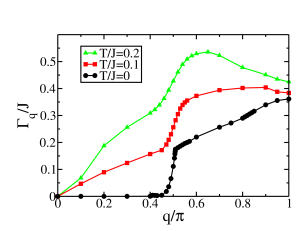
Figure 13: (Color online) Magnon linewidth $\Gamma_{q}$ (FWHM of $S(q,\omega)$) as a function of $q$, as obtained at $y=-1$ and temperatures $T/J=0$, 0.1 and 0.2. The lines are guides to the eye.

Finally, we analyze the variation of the FWHM with increasing temperature for a representative value of $y=-1$, see Fig. 13. At $T>0$ the thermal broadening at small momenta is clearly visible. As in the zero temperature case another strong increase of $\Gamma_{q}$ between $q=2\pi/5$ and $q=\pi/2$ is observed due to coupled spin-orbital degrees of freedom. For $T/J=0.1$ and $T/J=0.2$ we observe that $\Gamma_{q}$ has a temperature dependent maximum from where $\Gamma_{q}$ decreases towards the boundary of the Brillouin zone. This is due to the fact that the thermal broadening of the central peaks of the dynamic spin structure factor decreases from intermediate to high momenta (see Fig. 4). Actually without coupling to any orbital degrees of freedom we expect $\Gamma_{q}$ to be very small at the boundary of the Brillouin zone. Thus a large bandwidth at $q=\pi$ makes the spin-orbital model distinct from a pure 1D Heisenberg ferromagnet.

VI Thermodynamics

Coupled spin-orbital degrees of freedom will not only influence the spin dynamics but also the thermodynamics of the system. We expect, in particular, that the spin-orbital excitations which were shown to affect the dynamical spin structure factor in the previous section will also become observable in thermodynamic quantities when comparing the MF decoupling and the perturbative solution. In order to investigate this issue we rewrite Eq. (7) as

$$\mathcal{H}_{S\tau}(1)=H_{\textnormal{MF}}+\delta H,$$ (45)

with $\delta H=\mathcal{H}_{S\tau}(1)-H_{\textnormal{MF}}$. The MF part reads

$$H_{\textnormal{MF}}=\sum_{j=1}^{N} \left\{\mathcal{J}_{\tau}\left[\boldsymbol{\tau}_{j}\cdot\boldsymbol{\tau}_{j+1}\right]_{1}\right.\left.+\mathcal{J}_{S}\boldsymbol{S}_{j}\cdot\boldsymbol{S}_{j+1}\right.$$ (46)

$$\left.-\left<\boldsymbol{S}_{j}\cdot\boldsymbol{S}_{j+1}\right>_{\textnormal{MF}}\left<\left[\boldsymbol{\tau}_{j}\cdot\boldsymbol{\tau}_{j+1}\right]_{1}\right>_{\textnormal{MF}}\right\}.$$

The exchange constants $\mathcal{J}_{S,\tau}$ are defined in Eqs. (18).Rem We use the Hamiltonian (45) to determine the free energy per site perturbatively, following the expansion,

$$f=f^{S}_{\textnormal{MF}}+f^{\tau}_{\textnormal{MF}}+\frac{1}{N}\left<\delta H\right>_{\textnormal{MF}}^{c}\\ -\frac{1}{2NT}\left<\delta H^{2}\right>_{\textnormal{MF}}^{c}+\dots,$$ (47)

where $f_{\text{MF}}^{S}$ ($f_{\text{MF}}^{\tau}$) is the expression for the free energy per site stemming from the spin (pseudospin) sector within the MF decoupling solution. The subscript indicates that the respective correlation functions are calculated with $H_{\text{MF}}$. Moreover the superscript $c$ means that the above expansion of the free energy is restricted to connected diagrams. We note that Eq. (47) is a high temperature expansion valid if $|x|T/J\gg 1$ and $|y|T/J\gg 1$.

A straightforward calculation shows that the first order contribution only shifts the free energy, Eq. (47), and will not show up in thermodynamic observables obtained by taking derivatives of the free energy. For the second order contribution we have to evaluate two- and four-point correlation functions both for the spin and the pseudospin part.

Figure 14: Diagramatic representations of the second order contributions to the free energy as given by Eq. (50).

We use the abbreviations

$$\left<\left(\boldsymbol{S}_{j}\cdot\boldsymbol{S}_{j+1}\right)\left(\boldsymbol{S}_{l}\cdot\boldsymbol{S}_{l+1}\right)\right>=a+b(j,l)$$ (48)

for the spins and

$$\left<\left[\boldsymbol{\tau}_{j}\cdot\boldsymbol{\tau}_{j+1}\right]_{1}\left[\boldsymbol{\tau}_{l}\cdot\boldsymbol{\tau}_{l+1}\right]_{1}\right>=c+d(j,l)$$ (49)

for the pseudospins. Here the site-independent quantities $a$ and $c$ stand for the disconnected parts of the four-point correlation functions whereas $b(j,l)$ and $d(j,l)$ follow from the connected ones. One finds after a straightforward calculation that only the product of the connected parts contributes to the second order correction, leading to

$$\left<\delta H^{2}\right>_{\text{MF}}=J^{2}\sum_{j,l=1}^{N}b(j,l)d(j,l)\,.$$ (50)

To proceed further, we again apply the MSWT to the spin and a Jordan-Wigner transformation to the pseudospin part. The evaluation of $d(j,l)$ is again straightforward and yields

$$d(j,l) = \frac{1}{2N^{2}}\sum_{k_{1},k_{2}}n_{\text{F}}[\omega^{\text{MF}}_{\text{F}}(k_{1},0)]\{1-n_{\text{F}}[\omega^{\text{MF}}_{\text{F}}(k_{2},0)]\}$$

$$\hskip 19.91684pt\times\textnormal{e}^{i(k_{1}-k_{2})(j-l)}\left\{1+\cos(k_{1}+k_{2})\right\}$$

with $\omega^{\text{MF}}_{\text{F}}(q,\delta)$ as given in Eq. (21).

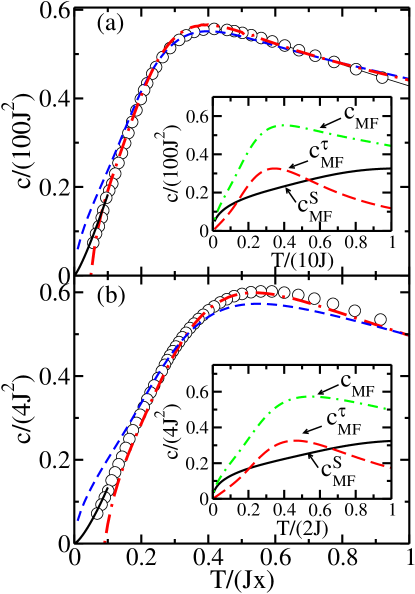
Figure 15: Specific heat per site $c/(Jx)^{2}$ as a function of $T/Jx$ for (a) $x=10$ and (b) $x=2$. The circles denote the numerical data from TMRG with the solid line obtained by a low-temperature fit of the TMRG data for the inner energy. The dashed lines correspond to MF decoupling while the dashed-dotted lines are the results obtained by perturbation theory. The perturbative results are expected to be valid for $1/x^{2}\ll T/(Jx)\ll 1$. Insets: Specific heat $c_{\text{MF}}$ within the MF solution (dashed-dotted line) with the contributions from the spin ($c_{\text{MF}}^{S}$ solid line) and the orbital ($c_{\text{MF}}^{\tau}$ dashed line) sector shown separately.

The evaluation of Eq. (48) is more involved. We first apply a Dyson-Maleev transformation and treat the obtained expressions using Wick’s theorem. In addition, we also have to account for the constraint of nonzero magnetization at $T>0$ imposed by the MSWT. The corresponding diagrams are shown in Fig. 14. Within this approximation the specific heat per site reads

$$c=c_{\text{MF}}+c_{2}+\dots\,,$$ (52)

with

$$c_{2}=J^{2}T\frac{\partial^{2}}{\partial T^{2}}\frac{\sum\limits_{j,l=1}^{N}b(j,l)d(j,l)}{2NT}\,.$$ (53)

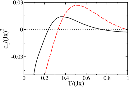
Figure 16: (Color online) Perturbative contribution to the specific heat per site $c_{2}/(Jx)^{2}$, Eq. (53), as a function of $T/Jx$ for $x=10$ (solid line) and $x=2$ (dashed line).

We calculate the first term in Eq. (52) within the MF decoupling, $c_{\text{MF}}=c_{\text{MF}}^{S}+c_{\text{MF}}^{\tau}$, from the internal energy which is determined by the respective nearest-neighbor correlation functions allowing us to keep terms up to quartic order in the bosonic operators.Herzog et al. (2010) This strategy makes it possible to obtain reliable results for $c_{\textnormal{MF}}^{S}$ up to $T/(|J_{S}|S^{2})\leq 1$. The second order correction $c_{2}$ given in Eq. (53) is obtained using the Dyson-Maleev transformation so that quartic terms are also included and the order of approximation is the same. Since we are using a high temperature expansion, Eq. (47), in combination with the MSWT to evaluate the diagrams, our results are only valid in an intermediate temperature regime. If we restrict ourselves to parameters $x=-y>0$ then this temperature range is given by $1/x\ll T/J\ll xS^{2}$. In the following we therefore only consider the case $x\gg 1$ and compare the results from perturbation theory with numerical data obtained by TMRG.

As shown in Fig. 15, the specific heat $c/(Jx)^{2}$ exhibits a broad maximum which corresponds to the characteristic energies of spin and fermionic particle-hole excitations. In the temperature range where the perturbative approach is valid we find excellent agreement with the numerical solution. In particular, the perturbative correction $c_{2}$ (see Fig. 16) correctly captures the weight shift from low to intermediate temperatures visible when comparing the numerical and the MF decoupling solution. In spite of this weight shift, the MF decoupling yields overall a very reasonable description of the specific heat for both cases shown in Fig. 15. For $x=10$, (Fig. 15(a)) the specific heat $c$ has a broad maximum at $T/(Jx)\simeq 0.4$. This maximum results from a distinct maximum in the orbital contribution $c_{\text{MF}}^{\tau}$, see insets in Fig. 15. In contrast the spin contribution $c_{\text{MF}}^{S}$ increases steadily with increasing temperature, in agreement with the higher energy scale for spin excitations. As a result, the total specific heat has only a weaker and broader maximum than suggested by the orbital part.

The MF decoupling does seem to fail, however, at very low temperatures. Here the MF solution predicts that spin excitations give the dominant contribution leading to a $c(T)\sim\sqrt{T}$ behavior. This is in contrast to an extrapolation of the numerical data shown as dot-dashed lines in Fig. 15 which suggests an approximately linear dependence on temperature. This discrepancy comes as a surprise because our perturbative calculations of the dynamical spin-structure factor in Sec. V.2 lead us to the conclusion that the magnons survive as sharp quasiparticles at low energies. More generally, one might argue that the ground state does not show any entanglement between the two sectors because of the classical nature of the FM state thus allowing for spin-wave excitations at low energies. From the point of view of a low-energy effective field theory, however, the situation is much less clear. While a FM chain is described by a low-energy effective theory with dynamical critical exponent $z=2$, the fermionic orbital chain has $z=1$. A coupling of spatial spin deviations to time-dependent orbital fluctuations then seems to require that the low-energy effective theory for the coupled system has $z=1$. As a consequence the temperature dependence of $c(T)$ would indeed be linear. However, such an approach leaves open the role and treatment of the Berry phase terms.

Within the perturbative approach the open question is whether or not higher order contributions to the self-energy might induce a significant broadening of the dynamical spin-structure factor also at low energies. In this regard we note that the vertex responsible for the broadening of $S(q,\omega)$ studied in Sec. V.2 does not play any role for the thermodynamics of the system. Here the constraint of vanishing magnetization means that such diagrams do not contribute to static correlation functions so that the lowest order corrections are caused by the vertex shown in Fig. 14.

VII Conclusions

In summary, we have investigated coupled spin-orbital degrees of freedom in a one-dimensional model. For ferromagnetic exchange we have shown that the considered model at special points in parameter space can be written in terms of Dirac exchange operators for spin $S$ and pseudospin $\tau$. As a consequence, three collective excitations of spin, orbital and coupled spin-orbital type do exist. In particular, we discussed the case of Dirac exchange operators for $S=\tau=1/2$ where the dispersions of all three elementary excitations are degenerate and lie within the spin-orbital continuum. While the spin-orbital excitations stay confined in this case, a decay becomes possible once we move away from this special point.

For antiferromagnetic exchange the one-dimensional spin-orbital model captures fundamental aspects of physics relevant for transition metal oxides and, as we have shown, sharp excitations do not exist. To address the question how the spin dynamics is influenced by fluctuating orbitals we considered the extreme quantum limit of orbitals interacting via an XY-type coupling. This allowed us to map the orbital sector onto free fermions using the Jordan-Wigner transformation. In spin-wave theory the spin sector is described by bosons so that our model corresponds to an effective boson-fermion model which applies for low temperatures. An analytic calculation of the properties within a mean-field decoupling approach is then straightforward. Compared to a numerical phase diagram based on the density-matrix renormalization group we find that the regime with ferromagnetically polarized spins is stabilized by the decoupling procedure. Furthermore, the mean-field decoupling gives rise to a finite temperature dimerized phase for certain parameters when starting from the ferromagnetic ground state. While a phase with long-range dimer order at finite temperatures is not possible in a purely one-dimensional model, the mean-field approach also completely ignores any kind of coupled spin-orbital excitations.

Thus we developed a self-consistent perturbative scheme to explore the role played by spin-orbital coupling. In perturbation theory the boson-fermion interaction does not produce any infrared divergencies in the one-dimensional model due to the lack of nesting. This makes a perturbative calculation of the spin structure factor $S(q,\omega)$ possible. At large momenta $q$, we find that $S(q,\omega)$ shows a significant broadening due to scattering of magnons by orbital excitations. For small momenta, on the other hand, no broadening in this lowest order perturbative approach is observed because the magnon cannot scatter on these excitations. The onset of the broadening occurs at momenta where the magnon enters the boson-fermion spectrum. This point, as well as details of the full width at half maximum is determined by the strength of interaction. Most interestingly, $S(q,\omega)$ does show additional peaks and shoulders corresponding to characteristic spin-orbital excitations. At points where the renormalized spin-wave dispersion and the dispersion of these excitations cross, Kohn anomalies do occur.

Furthermore, we compared numerical data for the specific heat of the spin-orbital model with the mean-field decoupling solution and an approach where we also took the second order correction to the mean-field result into account. Overall, we found that the mean-field decoupling does describe the specific heat reasonably well. A redistribution of entropic weight from low to intermediate temperatures observed when comparing the numerical data and the mean-field solution is very well captured by the second order perturbative correction. An interesting open point is the behavior of the specific heat $c(T)$ at low temperatures. While the mean-field solution predicts $c(T)\sim\sqrt{T}$ due to spin-wave excitations, the numerical data suggest instead that $c(T)\sim T$. We have speculated that a coupling of the two sectors might indeed lead to a low-energy effective theory with dynamical critical exponent $z=1$ but details of such a theory need to be worked out in the future.

In conclusion, we have shown that while collective spin-orbital excitations with infinite lifetime do not exist for antiferromagnetic superexchange the coupled spin-orbital degrees of freedom have a strong influence on the spin excitation spectrum as well as on the thermodynamic properties of the system. However, the treatment of spin-orbital systems beyond the range of validity of mean-field decoupling and perturbative schemes remains an open problem in theory.

Appendix A Details of the perturbative approach for the boson-fermion model

We start by a MF decoupling, rewriting the interaction as

$$H_{1}=H_{1,\text{MF}}+\underbrace{(H_{1}-H_{1,\text{MF}})}_{\delta H},$$

with

$$H_{1,\text{MF}}= \frac{1}{N^{2}}\sum_{k}\omega_{\text{BF}}(k,k,q)^{2}\left[\tilde{n}_{\text{b},k}f_{q}^{\dagger}f_{q}^{\ }+\tilde{n}_{\text{f},q}b_{k}^{\dagger}b_{k}^{\ }\right].$$

We treat $\delta H$ as perturbation. The averages $\tilde{n}_{\text{a},p}=\bigl{<}a_{p}^{\dagger}a_{p}^{\ }\bigr{>}$ are determined self-consistently within this MF scheme. This leads to a renormalization of the magnon and fermion dispersions. We find

$$\zeta(q)=2JS\left(|y|-\frac{1}{N}\sum_{k}\cos k\ \tilde{n}_{\text{f},k}\right)(1-\cos q)-\mu,$$ (54)

and

$$\omega_{\text{F}}(q)=\left(S^{2}+x+\frac{2}{N}\sum_{k}(1-\cos k)\tilde{n}_{\text{b},k}\right)\cos q.$$ (55)

For $T=0$ only the magnon dispersion is renormalized to

$$\zeta(q)=2JS(|y|+1/\pi)(1-\cos q).$$

By virtue of Dyson’s equation we may calculate the bosonic Green’s function at $T=0$.Fetter and Walecka (1971) Since the MF decoupling already takes the first order contributions into account, the lowest order diagrams we obtain are of second order. The self energy is thus approximated by the proper self-energy obtained by summing up those diagrams which may be composed by the second order diagrams. From this we have $\Sigma(q,\omega)\approx\Sigma_{2}(q,\omega)\equiv\Sigma_{\text{BF}}^{+}(q,\omega)+\Sigma_{\text{BF}}^{-}(q,\omega)+\Sigma_{2,1}(q)$ where the diagrams are given by $\Sigma_{\text{BF}}^{+}(q,\omega)$ (Fig. 6(a)), $\Sigma_{\text{BF}}^{-}(q,\omega)$ (Fig. 6(b)), and $\Sigma_{2,1}(q)$ (Fig. 6(c)). A straigthforward calculation reveals that at zero temperature $\Sigma_{2,1}(q)$ and $\Sigma_{\text{BF}}^{-}(q,\omega)$ vanish. For $\Sigma_{\text{BF}}^{+}(q,\omega)$ we find the expression given in Eq. (39).

For finite temperatures we calculate the imaginary time Green’s function. We find

$$\Sigma_{\text{BF}}^{\pm}(q,\omega_{\nu,\textnormal{B}}) =-\frac{T^{2}}{N^{2}}\sum_{k_{1},k_{2}}\omega_{\text{BF}}^{2}(q,k_{1},k_{2})$$ (56)

$$\times\sum_{a,b}\mathcal{G}^{(0)}_{\textnormal{F}}(k_{2},\omega_{a,\textnormal{F}})\mathcal{G}_{\textnormal{F}}^{(0)}(q-k_{1}+k_{2},\omega_{b,\textnormal{F}})$$

$$\times\mathcal{G}^{(0)}_{\textnormal{B}}(k_{1},\pm(\omega_{\nu,\textnormal{B}}-\omega_{b,\textnormal{F}}+\omega_{a,\textnormal{F}}))$$

for the diagrams in Fig. 6(a,b), and

$$\Sigma_{2,1}(q)= -\frac{T^{2}}{N^{2}}\sum_{k_{1},k_{2}}\omega_{\text{BF}}(q,q,k_{1})\omega_{\text{BF}}(k_{2},k_{2},k_{1})$$ (57)

$$\times\sum_{a,b}\left[\mathcal{G}_{\textnormal{F}}^{(0)}(k_{1},\omega_{a,\textnormal{F}})\right]^{2}\mathcal{G}_{\textnormal{B}}^{(0)}(k_{2},\omega_{b,\textnormal{B}})$$

for the diagram given in Fig. 6(c). Here we have used $\mathcal{G}_{\textnormal{F}}^{(0)}(q,\omega_{\mu,\textnormal{F}})=(i\omega_{\mu,\textnormal{F}}-\omega_{F}(q))^{-1}$ and $\mathcal{G}_{\textnormal{B}}^{(0)}(q,\omega_{\nu,\textnormal{B}})=(i\omega_{\nu,\textnormal{B}}-\zeta(q))^{-1}$ as the fermionic and bosonic Matsubara Green’s function for the noninteracting Hamiltonian, respectively. $\omega_{\nu,\textnormal{F}}$ are the fermionic Matsubara frequencies. After performing the frequency sums we end up with

$$\Sigma_{2,1}(q)= -\frac{1}{TN^{2}}\sum_{k_{1},k_{2}}\omega_{\text{BF}}(q,q,k_{1})\omega_{\text{BF}}(k_{2},k_{2},k_{1})$$ (58)

$$\times n_{\textnormal{B}}[\zeta(k_{2})](1-n_{\textnormal{F}}[\omega_{\text{F}}(k_{1})])n_{\textnormal{F}}[\omega_{\text{F}}(k_{1})],$$

and the self-energies $\Sigma_{\text{BF}}^{\pm}(q,\omega_{\nu,\text{B}})$ as given in Eqs. (V.1) and (43).

References

- Landau (1933) L. D. Landau, Phys. Z. Sowjetunion 3, 664 (1933).
- Fröhlich (1954) H. Fröhlich, Advances in Physics 3, 325 (1954).
- Peierls (1955) R. E. Peierls, Quantum Theory of Solids (Oxford University Press, Oxford, 1955).
- Das (2003) K. K. Das, Phys. Rev. Lett. 90, 170403 (2003).
- Albus et al. (2003) A. Albus, F. Illuminati, and J. Eisert, Phys. Rev. A 68, 023606 (2003).
- Cazalilla and Ho (2003) M. A. Cazalilla and A. F. Ho, Phys. Rev. Lett. 91, 150403 (2003).
- Mathey et al. (2004) L. Mathey, D.-W. Wang, W. Hofstetter, M. D. Lukin, and E. Demler, Phys. Rev. Lett. 93, 120404 (2004).
- Lewenstein et al. (2004) M. Lewenstein, L. Santos, M. A. Baranov, and H. Fehrmann, Phys. Rev. Lett. 92, 050401 (2004).
- Kugel and Khomskii (1980) K. I. Kugel and D. I. Khomskii, Sov. Phys. JETP 52, 501 (1980).
- Feiner and Oleś (1999) L. F. Feiner and A. M. Oleś, Phys. Rev. B 59, 3295 (1999).
- Tokura and Nagaosa (2000) Y. Tokura and N. Nagaosa, Science 288, 462 (2000).
- Tokura (2000) Colossal Magnetoresistive Oxides, edited by Y. Tokura, (Gordon and Breach, Amsterdam, 2000).
- Kovaleva et al. (2010) N. N. Kovaleva, A. M. Oleś, A. M. Balbashov, A. Maljuk, D. N. Argyriou, G. Khaliullin, and B. Keimer, Phys. Rev. B 81, 235130 (2010).
- Khaliullin and Maekawa (2000) G. Khaliullin and S. Maekawa, Phys. Rev. Lett. 85, 3950 (2000).
- Keimer et al. (2000) B. Keimer, D. Casa, A. Ivanov, J. W. Lynn, M. v. Zimmermann, J. P. Hill, D. Gibbs, Y. Taguchi, and Y. Tokura, Phys. Rev. Lett. 85, 3946 (2000).
- Hemberger et al. (2003) J. Hemberger, H.-A. K. von Nidda, V. Fritsch, J. Deisenhofer, S. Lobina, T. Rudolf, P. Lunkenheimer, F. Lichtenberg, A. Loidl, D. Bruns, and B. Büchner, Phys. Rev. Lett. 91, 066403 (2003).
- Cwik et al. (2003) M. Cwik, T. Lorenz, J. Baier, R. Müller, G. André, F. Bourée, F. Lichtenberg, A. Freimuth, R. Schmitz, E. Müller-Hartmann, and M. Braden, Phys. Rev. B 68, 060401 (2003).
- Ren et al. (1998) Y. Ren, T. T. M. Palstra, D. I. Khomskii, A. A. Nugroho, A. A. Menovsky, and G. A. Sawatzky, Nature (London) 396, 441 (1998).
- Ren et al. (2000) Y. Ren, T. T. M. Palstra, D. I. Khomskii, A. A. Nugroho, A. A. Menovsky, and G. A. Sawatzky, Phys. Rev. B 62, 6577 (2000).
- Noguchi et al. (2000) M. Noguchi, A. Nakazawa, S. Oka, T. Arima, Y. Wakabayashi, H. Nakao, and Y. Murakami, Phys. Rev. B 62, R9271 (2000).
- Khaliullin et al. (2001) G. Khaliullin, P. Horsch, and A. M. Oleś, Phys. Rev. Lett. 86, 3879 (2001).
- Ulrich et al. (2003) C. Ulrich, G. Khaliullin, J. Sirker, M. Reehuis, M. Ohl, S. Miyasaka, Y. Tokura, and B. Keimer, Phys. Rev. Lett. 91, 257202 (2003).
- Horsch et al. (2003) P. Horsch, G. Khaliullin, and A. M. Oleś, Phys. Rev. Lett. 91, 257203 (2003).
- Sirker and Khaliullin (2003) J. Sirker and G. Khaliullin, Phys. Rev. B 67, 100408 (2003).
- Horsch et al. (2008) P. Horsch, G. Khaliullin, A. M. Oleś, and L. F. Feiner, Phys. Rev. Lett. 100, 167205 (2008).
- Sirker et al. (2008) J. Sirker, A. Herzog, A. M. Oleś, and P. Horsch, Phys. Rev. Lett. 101, 157204 (2008).
- Oleś et al. (2006) A. M. Oleś, P. Horsch, L. F. Feiner, and G. Khaliullin, Phys. Rev. Lett. 96, 147205 (2006).
- Itoi et al. (2000a) C. Itoi, S. Qin, and I. Affleck, Phys. Rev. B 61, 6747 (2000a).
- Sirker (2004) J. Sirker, Phys. Rev. B 69, 104428 (2004).
- van den Brink et al. (1998) J. van den Brink, W. Stekelenburg, D. I. Khomskii, G. A. Sawatzky, and K. I. Kugel, Phys. Rev. B 58, 10276 (1998).
- Li et al. (1998) Y. Q. Li, M. Ma, D. N. Shi, and F. C. Zhang, Phys Rev Lett 81, 3527 (1998).
- rem (a) This is reminiscent to the SU(4) model with AF exchange where all three elementary excitations are degenerate. However in the latter case the elementary excitations are of coupled spin-orbital type, whereas in the present case we find elementary spin, orbital and combined spin-orbital excitations.
- (33) This, we believe, is a consequence of a factor of missed in the analysis of the elementary dispersions in this work.
- Dirac (1958) P. A. M. Dirac, Principles of Quantum Mechanics (Oxford University Press, Oxford, 1958).
- Schrödinger (1941) E. Schrödinger, Proceedings of the Royal Irish Academy Section A 47, 39 (1941).
- Brown (1985) H. A. Brown, Phys. Rev. B 31, 3118 (1985).
- Feiner et al. (1998) L. F. Feiner, A. M. Oleś, and J. Zaanen, J. Phys.: Condens. Matter 10, L555 (1998).
- Oleś et al. (2000) A. M. Oleś, L. F. Feiner, and J. Zaanen, Phys. Rev. B 61, 6257 (2000).
- Takahashi (1990) M. Takahashi, Phys. Rev. B 42, 766 (1990).
- Takahashi (1993) M. Takahashi, Phys. Rev. B 47, 8336 (1993).
- Takahashi (1987) M. Takahashi, Phys. Rev. Lett 58, 168 (1987).
- Takahashi (1986) M. Takahashi, Prog. Theor. Phys. Suppl. 87, 233 (1986).
- Mizokawa and Fujimori (1996) T. Mizokawa and A. Fujimori, Phys. Rev. B 54, 5368 (1996).
- Sawada and Terakura (1998) H. Sawada and K. Terakura, Phys. Rev. B 58, 6831 (1998).
- Mizokawa et al. (1999) T. Mizokawa, D. I. Khomskii, and G. A. Sawatzky, Phys. Rev. B 60, 7309 (1999).
- Park et al. (2000) J.-H. Park, L. H. Tjeng, A. Tanaka, J. W. Allen, C. T. Chen, P. Metcalf, J. M. Honig, F. M. F. de Groot, and G. A. Sawatzky, Phys. Rev. B 61, 11506 (2000).
- Bursill et al. (1996) R. J. Bursill, T. Xiang, and G. A. Gehring, J. Phys. Cond. Mat. 8, L583 (1996).
- Wang and Xiang (1997) X. Wang and T. Xiang, Phys Rev B 56, 5061 (1997).
- Sirker and Klümper (2002) J. Sirker and A. Klümper, Europhys. Lett. 60, 262 (2002).
- White and Huse (1993) S. R. White and D. S. Huse, Phys. Rev. B 48, 3844 (1993).
- Miyashita and Kawakami (2005) S. Miyashita and N. Kawakami, J. Phys. Soc. Japan 74, 758 (2005).
- Itoi et al. (2000b) C. Itoi, S. Qin, and I. Affleck, Phys. Rev. B 61, 6747 (2000b).
- Chen et al. (2007) Y. Chen, Z. D. Wang, Y. Q. Li, and F. C. Zhang, Phys. Rev. B 75, 195113 (2007).
- Herzog et al. (2010) A. Herzog, P. Horsch, A. M. Oleś, and J. Sirker, Journal of Physics Conference Series 200, 022017 (2010).
- Pincus (1971) P. Pincus, Solid State Communications 9, 1971 (1971).
- rem (b) The discussion of the dynamical spin structure factor for the dimerized FM chain will be given elsewhere.
- FT (0) We note that the MF decoupling applied to the interaction given in Eq. (14) does not renormalize the dispersion of the fermions at .
- Giamarchi (2003) T. Giamarchi, Quantum Physics in One Dimension (Clarendon Press, Oxford, 2003).
- Metzner et al. (1998) W. Metzner, C. Castellani, and C. D. Castro, Advances in Physics 47, 317 (1998).
- Kohn (1959) W. Kohn, Phys. Rev. Lett. 2, 393 (1959).
- Woll and Nettel (1961) E. J. Woll and S. J. Nettel, Phys. Rev. 123, 769 (1961).
- Barnea and Horwitz (1975) G. Barnea and G. Horwitz, J. Phys. C 8, 2124 (1975).
- Møller and Houmann (1966) H. B. Møller and J. C. G. Houmann, Phys. Rev. Lett. 16, 737 (1966).
- Halilov et al. (1998) S. V. Halilov, H. Eschrig, A. Y. Perlov, and P. M. Oppeneer, Phys. Rev. B 58, 293 (1998).
- Pajda et al. (2001) M. Pajda, J. Kudrnovský, I. Turek, V. Drchal, and P. Bruno, Phys. Rev. B 64, 174402 (2001).
- Morán et al. (2003) S. Morán, C. Ederer, and M. Fähnle, Phys. Rev. B 67, 012407 (2003).
- (67) Performing the MF decoupling with the Hamiltonian (7) also takes the quartic orders of the Dyson-Maleev transformation into account. These higher orders are neglected in the MF decoupling performed in Sec. V. For low temperatures, i.e. the temperature region we have used in Sec. V the contributions from these higher order terms are small.
- Fetter and Walecka (1971) A. L. Fetter and J. D. Walecka, Quantum Theory of Many-Particle Sytems (McGraw-Hill, Inc., New York, 1971).