Special Geometries Emerging from Yang-Mills Type Matrix Models

Abstract:

I review some recent results which demonstrate how various geometries, such as Schwarzschild and Reissner-Nordström, can emerge from Yang-Mills type matrix models with branes. Furthermore, explicit embeddings of these branes as well as appropriate Poisson structures and star-products which determine the non-commutativity of space-time are provided. These structures are motivated by higher order terms in the effective matrix model action which semi-classically lead to an Einstein-Hilbert type action.

1 Background

In past years, various approaches to quantum space-time have been pursued. One possibility is to replace classical space-time by a %2CnNuovo Cim.  (o) ne where the coordinate functions $x^{\mu}$ are promoted to Hermitian operators $X^{\mu}$ on a Hilbert space $\mathcal{H}$. These “coordinate” operators satisfy certain non-trivial commutation relations

$$[X^{\mu},X^{\nu}]=\textrm{i}\theta^{\mu\nu}\,,$$ (1)

which in the simplest case reduce to a Heisenberg algebra, i.e. with constant $\theta^{\mu\nu}$. For a review of such %2CiNuovo Cim.  (f) ield theories see e.g. [1, 2, 3, 4]. In order to incorporate gravity in this context, however, a dynamical non-constant commutator $\theta^{\mu\nu}$ is required, which semi-classically determines a Poisson structure on space-time. Incidentally, matrix models of Yang-Mills type naturally realize this idea — for a review, see [7] and [9, 10, 11]. Our starting point is hence the matrix model action

$$S_{YM} =-{\rm Tr}[X^{a},X^{b}][X^{c},X^{d}]\eta_{ac}\eta_{bd}\,,$$ (2)

where $\eta_{ab}$ denotes the flat metric of a $D$-dimensional embedding space with arbitrary signature and $X^{a}$ are Hermitian matrices on $\mathcal{H}$ which in the semi-classical limit are interpreted as coordinate functions. If one considers some of the coordinates to be functions of the remaining ones [12] such that $X^{a}\sim x^{a}=(x^{\mu},\phi^{i}(x^{\mu}))$ in the semi-classical limit, one can interpret the $x^{a}$ as defining the embedding of a $2n$-dimensional submanifold ${\cal M}^{2n}\hookrightarrow\mathds{R}^{D}$ equipped with a non-trivial induced metric

$$g_{\mu\nu}(x) =\partial_{\mu}x^{a}\partial_{\nu}x^{b}\eta_{ab}=\eta_{\mu\nu}+\partial_{i}\phi^{i}(x)\partial_{j}\phi^{j}(x)\,,$$ (3)

via pull-back of $\eta_{ab}$, and where $\mu,\nu\in{1,\ldots,2n}$ and $i,j\in{2n+1,\ldots,D}$. Here we consider this submanifold to be a four dimensional space-time ${\cal M}^{4}$, and following [12] we can interpret

$$-\textrm{i}[X^{\mu},X^{\nu}]\sim\{x^{\mu},x^{\nu}\}_{pb}=\textrm{i}\theta^{\mu\nu}(x)$$ (4)

as a Poisson structure on ${\cal M}^{4}$. Furthermore, we assume that $\theta^{\mu\nu}$ is non-degenerate, so that its inverse matrix $\theta^{-1}_{\mu\nu}$ defines a symplectic form

$$\varTheta=\frac{1}{2}\theta^{-1}_{\mu\nu}dx^{\mu}\wedge dx^{\nu}$$ (5)

on ${\cal M}^{4}$. However, it is not the induced metric which is “seen” by scalar fields, gauge fields, etc., but the effective metric [9]

$$G^{\mu\nu} =e^{-\sigma}\theta^{\mu\rho}\theta^{\nu\sigma}g_{\rho\sigma}\,, e^{-\sigma} \equiv\frac{\sqrt{\det\theta^{-1}_{\mu\nu}}}{\sqrt{\det G_{\rho\sigma}}}\,.$$ (6)

Therefore, an interesting special case where $G_{\mu\nu}=g_{\mu\nu}$ may be considered. In fact, this corresponds to having a (anti-) self-dual symplectic form, i.e. $\star\varTheta=\pm\textrm{i}\varTheta$. This case, however is restricted to 4-dimensional submanifolds ${\cal M}^{4}$, as in four dimensions one always has $|G|=|g|$ which makes the assumptions above possible. (For details, see [7].) Let us consider the following example in order to make the effective geometry clearer: The gauge invariant kinetic term of a test particle modelled by a scalar field $\phi$ has the form

$$S[\phi] =-{\rm Tr}[X^{a},\Phi][X^{b},\Phi]\eta_{ab}$$

$$\sim\int\!\!d^{4}x\sqrt{\det\theta^{-1}}\theta^{\mu\nu}\partial_{\mu}x^{a}\partial_{\nu}\phi\theta^{\rho\sigma}\partial_{\rho}x^{b}\partial_{\sigma}\phi\eta_{ab}$$

$$=\int\!\!d^{4}x\sqrt{\det\theta^{-1}}G^{\nu\sigma}\partial_{\nu}\phi\partial_{\sigma}\phi\,.$$ (7)

2 Curvature

Figure 1: Embedding and induced metric

The bare matrix model Eqn. (2) without matter leads to the following e.o.m. for $X^{c}$:

$$[X^{a},[X^{b},X^{c}]]\eta_{ab} =0\,.$$ (8)

Furthermore, one can derive the matrix energy-momentum tensor $T^{ab}$ which reads [13, 14]

$$T^{ab} =H^{ab}-\frac{1}{4}\eta^{ab}H\,\sim\,\,e^{\sigma}\left(\frac{(Gg)}{4}\eta^{ab}-G^{\mu\nu}\partial_{\mu}x^{a}\partial_{\nu}x^{b}\right)\,,$$

$$H^{ab} =\frac{1}{2}[[X^{a},X^{c}],[X^{b},X_{c}]]_{+}\sim\,\,-e^{\sigma}G^{\mu\nu}\partial_{\mu}x^{a}\partial_{\nu}x^{b}\,,$$

$$H =H^{ab}\eta_{ab}\,,$$ (9)

and whose conservation follows directly from the matrix equations of motion (8) above:

$$[X^{a},T^{a^{\prime}b}]\eta_{aa^{\prime}}=0\,.$$ (10)

Interestingly, there is a close connection between the matrix energy-momentum tensor and the projectors on the tangential/normal bundle of ${\cal M}\in\mathds{R}^{D}$

$${\cal P}^{ab}_{T} =g^{\mu\nu}\partial_{\mu}x^{a}\partial_{\nu}x^{b}\,, {\cal P}^{ab}_{N} =\eta^{ab}-{\cal P}^{ab}_{T}\,.$$ (11)

Namely, in the special case where both metrics coincide, i.e. the self-dual case where $G_{\mu\nu}=g_{\mu\nu}$, one has $T^{ab}\sim e^{\sigma}{\cal P}_{N}^{ab}$ and $H^{ab}\sim-e^{\sigma}{\cal P}_{T}^{ab}$ in the semi-classical limit. Furthermore, one easily derives the relation $\nabla^{g}_{\sigma}\nabla^{g}_{\nu}x^{a}={\cal P}^{ab}_{N}\nabla^{G}_{\sigma}\nabla^{G}_{\nu}x_{b}$, where $\nabla^{g}/\nabla^{G}$ are the covariant derivatives defined with standard Christoffel symbols with respect to $g/G$, respectively. Hence the curvature tensor with respect to the induced metric $g$ can be written as

$$R_{\rho\sigma\nu\mu}[g] =\nabla^{g}_{\sigma}\nabla^{g}_{\mu}x^{a}\nabla^{g}_{\rho}\nabla^{g}_{\nu}x_{a}-\nabla^{g}_{\sigma}\nabla^{g}_{\nu}x^{a}\nabla^{g}_{\mu}\nabla^{g}_{\rho}x_{a}$$

$$={\cal P}_{N}^{ab}\nabla^{G}_{\sigma}\nabla^{G}_{\mu}x_{a}\nabla^{G}_{\rho}\nabla^{G}_{\nu}x_{b}-{\cal P}_{N}^{ab}\nabla^{G}_{\sigma}\nabla^{G}_{\nu}x_{a}\nabla^{G}_{\mu}\nabla^{G}_{\rho}x_{b}\,,$$ (12)

where the first line is simply the Gauss-Codazzi theorem, and Latin indices were pulled down with the embedding metric $\eta_{ab}$. Using the tensor $C_{\alpha;\mu\nu}:=\partial_{\alpha}x^{a}\nabla^{G}_{\mu}\partial_{\nu}x_{a}$ allows to relate the curvature tensors associated with $G/g$:

$$R_{\rho\sigma\nu\mu}[g] =(Gg)^{\eta}_{\mu}R_{\rho\sigma\nu\eta}[G]+\nabla^{G}_{\sigma}C_{\mu;\rho\nu}-\nabla^{G}_{\rho}C_{\mu;\sigma\nu}-C_{\alpha;\sigma\mu}C_{\beta;\rho\nu}g^{\alpha\beta}+C_{\alpha;\sigma\nu}C_{\beta;\mu\rho}g^{\alpha\beta}\,.$$ (13)

It was previously shown in [13, 14], that the Einstein-Hilbert action emerges in the effective matrix model action. In particular, a certain combination of order 10 matrix terms semi-classically leads to

$$S_{{\cal O}(X^{10})}\sim \,\int\!\!d^{4}x\frac{\sqrt{g}}{(2\pi)^{2}}e^{2\sigma}(R[g]-3R^{\mu\nu}[g]h_{\mu\nu})+{\cal O}(\partial h^{2})\,,$$

where $G_{\mu\nu}=g_{\mu\nu}+h_{\mu\nu}$ is almost self-dual. In the self-dual case (i.e. $h=0$), this reduces to

$$S_{{\cal O}(X^{10})}={\rm Tr}\left(2T^{ab}\Box X_{a}\Box X_{b}-T^{ab}\Box H_{ab}\right)\sim-2\!\int\!d^{4}x\sqrt{g}\,e^{2\sigma}R\,,$$ (14)

where $\Box Y\equiv[X^{a},[X_{a},Y]]$, and additionally one finds the order 6 matrix terms

$$S_{{\cal O}(X^{6})} ={\rm Tr}\left(\frac{1}{2}[X^{c},[X^{a},X^{b}]][X_{c},[X_{a},X_{b}]]-\Box X^{a}\Box X_{a}\right)$$

$$\sim\int\!d^{4}x\sqrt{g}\,\bigg{(}\frac{1}{2}\theta^{\mu\rho}\theta^{\eta\alpha}R_{\mu\rho\eta\alpha}-2e^{\sigma}R+2e^{\sigma}\partial^{\mu}\sigma\partial_{\mu}\sigma\!\bigg{)}.$$ (15)

In general, however, the degrees of freedom are given by the embedding $\phi^{i}$ and the deviation from the self-dual Poisson structure $A_{\mu}$, i.e.:

$$\theta^{-1}_{\mu\nu} =\bar{\theta}^{-1}_{\mu\nu}+F_{\mu\nu}=\bar{\theta}^{-1}_{\mu\nu}+\partial_{\mu}A_{\nu}-\partial_{\nu}A_{\mu}\,,$$

$$\delta_{\phi}g_{\mu\nu} =\delta\phi^{i}\phi^{j}\eta_{ij}+\phi^{i}\delta\phi^{j}\eta_{ij}\,,$$

$$\delta_{A}F_{\mu\nu} =\partial_{\mu}\delta A_{\nu}-\partial_{\nu}\delta A_{\mu}\,,$$

$$h_{\mu\nu} =-e^{\bar{\sigma}}(\bar{\theta}^{-1}gF)_{\mu\nu}-e^{\bar{\sigma}}(Fg\bar{\theta}^{-1})_{\mu\nu}-\frac{1}{2}g_{\mu\nu}(\bar{\theta}F)+{\cal O}(F^{2})\,,$$ (16)

where $\bar{\theta}^{-1}_{\mu\nu}$ denotes a self-dual Poisson structure with respect to a given metric $g_{\mu\nu}(\phi^{i})$. It was in fact argued in [14], that the tree level action Eqn. (2) should single out almost self-dual geometries and that certain potential terms set the non-commutativity scale $e^{\sigma}\approx\,$const. In the following section, we will consider two examples of geometries which are expected to solve the e.o.m. of the effective matrix model (i.e. including higher order contributions) too a good approximation [15], at least at some distance from the horizons.

3 Special Geometries

3.1 Schwarzschild Geometry

We now continue with the special example of Schwarzschild geometry, and our construction involves two steps [15, 8]: First, the choice of a suitable embedding ${\cal M}^{4}\subset\mathds{R}^{D}$ must be made such that the induced geometry on ${\cal M}^{4}$ given by $g_{\mu\nu}$ is the Schwarzschild metric, and then on needs to find a suitable non-degenerate Poisson structure on ${\cal M}^{4}$ which solves the e.o.m. $\nabla^{\mu}\theta^{-1}_{\mu\nu}=0$ for self-dual symplectic form $\varTheta$. Both steps are far from unique a priori. However, the freedom is considerably reduced by requiring that the solution should be a “local perturbation” of an asymptotically flat (or nearly flat) “cosmological” background. This is clear on physical grounds, having in mind the geometry near a star in some larger cosmological context: It must be possible to approximately “superimpose” our solution, allowing e.g. for systems of stars and galaxies in a natural way. This eliminates the well-known embeddings of the Schwarzschild geometry in the literature [16, 17, 18], which are highly non-trivial for large $r$ and cannot be superimposed in any obvious way. Furthermore, the embedding should be asymptotically harmonic $\Box x^{a}\to 0$ for $r\to\infty$, in view of the fact that there may be terms in the matrix model which depend on the extrinsic geometry, and which typically single out such harmonic embeddings. Additionally, $\theta^{\mu\nu}$ should be non-degenerate, and $\theta^{\mu\nu}\to\textrm{const.}\neq 0$ as $r\to\infty$. We start by considering Eddington-Finkelstein coordinates and define:

$$t =t_{S}+(r^{*}-r)\,, r^{*} =r+r_{c}\ln\left|\frac{r}{r_{c}}-1\right|\,,$$ (17)

where $t_{S}$ denotes the usual Schwarzschild time, $r_{c}$ is the horizon of the Schwarzschild black hole and $r^{*}$ is the well-known tortoise coordinate. The metric in Eddington-Finkelstein coordinates $\{t,r,\vartheta,\varphi\}$ is given by

$$ds^{2} =-\left(1-\frac{r_{c}}{r}\right)dt^{2}+\frac{2r_{c}}{r}dtdr+\left(1+\frac{r_{c}}{r}\right)dr^{2}+r^{2}d\Omega^{2}\,,$$ (18)

which is asymptotically flat for large $r$, and manifestly regular at the horizon $r_{c}$ and thus allows us to find an embedding which fulfills the requirements listed above.

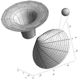
Figure 2: Embedded Schwarzschild black hole.

In particular, we need at least 3 extra dimensions:

$$\phi_{1}+i\phi_{2} =\phi_{3}e^{i\omega(t+r)}\,, \phi_{3} =\frac{1}{\omega}\sqrt{\frac{r_{c}}{r}}\,,$$ (19)

where $\phi_{3}$ is time-like and $\omega$ is some parameter which does not enter the metric (18). Hence, our 7-dimensional embedding is given by

$$x^{a} =\left(\begin{array}[]{c}t\\ r\cos\varphi\sin\vartheta\\ r\sin\varphi\sin\vartheta\\ r\cos\vartheta\\ \frac{1}{\omega}\sqrt{\frac{r_{c}}{r}}\cos\left(\omega(t+r)\right)\\[3.00003pt] \frac{1}{\omega}\sqrt{\frac{r_{c}}{r}}\sin\left(\omega(t+r)\right)\\[3.00003pt] \frac{1}{\omega}\sqrt{\frac{r_{c}}{r}}\end{array}\right)$$ (27)

with background metric $\eta_{ab}=\mbox{diag}(-,+,+,+,+,+,-)$. On the top of Fig. 2, a schematic view of the outer region of the Schwarzschild black hole is shown. After passing through the horizon $r=r_{c}$, the extra dimensions $\phi_{i}$ “blow up” in a cone-like manner. As indicated in the lower half of this figure, every point of the cone is in fact a sphere whose radius $r$ becomes smaller towards the bottom of the cone (i.e. $T\propto 1/\sqrt{r}$). The twisted vertical lines drawn in the cone are lines of equal time $t$. For the symplectic form, we require $\star\varTheta=i\varTheta$, so that the effective and the induced metric coincide, i.e. $G^{\mu\nu}=e^{\sigma}\theta^{\mu\rho}\theta^{\nu\sigma}g_{\rho\sigma}=g^{\mu\nu}$, and $\lim\limits_{r\to\infty}e^{-\sigma}=\textrm{const.}\neq 0$. One then finds the solution [15]

$$\varTheta =iE\wedge dt_{S}+B\wedge d\varphi\,,$$

$$E =c_{1}\left(\cos\vartheta dr-r\gamma\sin\vartheta d\vartheta\right)=d(f(r)\cos\vartheta)\,,$$

$$B =c_{1}\left(r^{2}\sin\vartheta\cos\vartheta d\vartheta+r\sin^{2}\vartheta dr\right)=\frac{c_{1}}{2}d(r^{2}\sin^{2}\vartheta)\,,$$

$$\gamma =\left(1-\frac{r_{c}}{r}\right)\,,\qquad f(r)=c_{1}r\gamma\,,\qquad f^{\prime}=c_{1}=\textrm{const.}\,,$$ (28)

from which follows

$$e^{-\sigma} =c_{1}^{2}\left(1-\frac{r_{c}}{r}\sin^{2}\vartheta\right)\equiv c_{1}^{2}e^{-\bar{\sigma}}\,,$$ (29)

where $c_{1}$ is an arbitrary constant. Clearly, near the horizon $e^{-\sigma}\approx\,$const. is not fulfilled, meaning our approximations break down in that region. Asymptotically, however, this seems to be a valid solution which approximately fulfills all requirements listed at the beginning of this section. Furthermore, Eqn. (28) suggests to work in Darboux coordinates $x_{D}^{\mu}=\{H_{ts},t_{S},H_{\varphi},\varphi\}$ corresponding to Killing vector fields $V_{ts}=\partial_{t_{s}}\,,\,V_{\varphi}=\partial_{\varphi}$ where the symplectic form $\varTheta$ is constant:

$$\varTheta =ic_{1}dH_{ts}\wedge dt_{S}+c_{1}dH_{\varphi}\wedge d\varphi\,,$$

$$=c_{1}d\left(iH_{ts}dt_{S}+H_{\varphi}d\varphi\right)\,,$$

$$H_{ts} =r\gamma\cos\vartheta\,,\qquad H_{\varphi}=\frac{1}{2}r^{2}\sin^{2}\vartheta\,.$$ (30)

The relations to the Killing vector fields are given by

$$E =c_{1}dH_{ts}=c_{1}E_{\mu}dx^{\mu}=i_{V_{ts}}\varTheta\,, E_{\mu}=V_{ts}^{\nu}\theta^{-1}_{\nu\mu}\,,$$

$$B =c_{1}dH_{\varphi}=c_{1}B_{\mu}dx^{\mu}=i_{V_{\varphi}}\varTheta\,, B_{\mu}=V_{\varphi}^{\nu}\theta^{-1}_{\nu\mu}\,,$$ (31)

and the metric in Darboux coordinates reads

$$ds_{D}^{2} =-\gamma dt_{S}^{2}+\frac{e^{\bar{\sigma}}}{\gamma}dH_{ts}^{2}+r^{2}\sin^{2}\vartheta d\varphi^{2}+\frac{e^{\bar{\sigma}}}{r^{2}\sin^{2}\vartheta}dH_{\varphi}^{2}\,.$$ (32)

Hence, a Moyal type star product can easily be defined as

$$(g\star h)(x_{D}) =g(x_{D})e^{-\frac{i}{2}\left(\overleftarrow{\partial}_{\mu}\theta_{D}^{\mu\nu}\overrightarrow{\partial}_{\nu}\right)}h(x_{D})\,, \textrm{with }\quad\theta_{D}^{\mu\nu} =\epsilon\left(\begin{array}[]{cccc}0&i&0&0\\ -i&0&0&0\\ 0&0&0&1\\ 0&0&-1&0\end{array}\right)\,,$$ (37)

where $\epsilon=1/c_{1}\ll 1$ denotes the expansion parameter. Transforming back to embedding coordinates, the star product reads

$$(g\star h)(x) =g(x)\exp\Bigg{[}\frac{\textrm{i}\epsilon}{2}\Bigg{(}\!\!\left(\overleftarrow{\partial}_{t}\frac{\textrm{i}r_{c}ze^{\bar{\sigma}}}{r^{2}\gamma}+\overleftarrow{\partial}_{z}\textrm{i}e^{\bar{\sigma}}\right)\wedge\overrightarrow{\partial}_{t}$$

$$\quad+\!\left(\!\left(\overleftarrow{\partial}_{t}\!-\!\overleftarrow{\partial}_{z}\frac{z}{r}\right)\!\frac{r_{c}e^{\bar{\sigma}}}{r^{2}}\!+\!\left(\overleftarrow{\partial}_{x}x+\overleftarrow{\partial}_{y}y\right)\!\frac{1}{x^{2}+y^{2}}\right)\!\wedge\!\left(x\overrightarrow{\partial}_{y}-y\overrightarrow{\partial}_{x}\right)\!\!\Bigg{)}\!\Bigg{]}h(x)$$ (38)

where the wedge stands for “antisymmetrized”, and when considering the expansion care must be taken with the sequence of operators and the side they act on. To leading order one hence finds the star commutators

$$-\textrm{i}\left[x^{a}\stackrel{{\scriptstyle\star}}{{,}}x^{b}\right] =\epsilon e^{\bar{\sigma}}\left(\!\!\!\begin{array}[]{ccccccc}0&-\frac{r_{c}y}{r^{2}}&\frac{r_{c}x}{r^{2}}&-\textrm{i}&\frac{\textrm{i}zf^{+}_{12}(1)}{r}&\frac{\textrm{i}zf^{-}_{21}(1)}{r}&\frac{\textrm{i}z\phi_{3}}{2r^{2}}\\ \frac{r_{c}y}{r^{2}}&0&e^{-\bar{\sigma}}&-\frac{r_{c}yz}{r^{3}}&\frac{-yf^{+}_{12}(\gamma)}{r}&\frac{-yf^{-}_{21}(\gamma)}{r}&-\frac{y\gamma\phi_{3}}{2r^{2}}\\ -\frac{r_{c}x}{r^{2}}&-e^{-\bar{\sigma}}&0&\frac{r_{c}xz}{r^{3}}&\frac{xf^{+}_{12}(\gamma)}{r}&\frac{xf^{-}_{21}(\gamma)}{r}&\frac{x\gamma\phi_{3}}{2r^{2}}\\ \textrm{i}&\frac{r_{c}yz}{r^{3}}&-\frac{r_{c}xz}{r^{3}}&0&-i\omega\phi_{2}&\textrm{i}\omega\phi_{1}&0\\ \!\!\frac{-\textrm{i}zf^{+}_{12}(1)}{r}&\frac{yf^{+}_{12}(\gamma)}{r}&\frac{-xf^{+}_{12}(\gamma)}{r}&i\omega\phi_{2}&0&-\frac{i\omega z\phi_{3}^{2}}{2r^{2}}&\frac{-i\omega z\phi_{3}\phi_{2}}{2r^{2}}\\ \!\!\frac{-\textrm{i}zf^{-}_{21}(1)}{r}&\frac{yf^{-}_{21}(\gamma)}{r}&\frac{-xf^{-}_{21}(\gamma)}{r}&-i\omega\phi_{1}&\frac{i\omega z\phi_{3}^{2}}{2r^{2}}&0&\frac{i\omega z\phi_{3}\phi_{1}}{2r^{2}}\\ -\frac{\textrm{i}z\phi_{3}}{2r^{2}}&\frac{y\gamma\phi_{3}}{2r^{2}}&-\frac{x\gamma\phi_{3}}{2r^{2}}&0&\frac{\textrm{i}\omega z\phi_{3}\phi_{2}}{2r^{2}}&\frac{-\textrm{i}\omega z\phi_{3}\phi_{1}}{2r^{2}}&0\end{array}\!\!\!\!\!\right)$$ (46)

$$\quad+{\cal O}(\epsilon^{3})\,,$$ (47)

where

$$f^{\pm}_{ij}(Y) =\left(\frac{Y}{2r}\phi_{i}\pm\omega\phi_{j}\right)\,.$$ (48)

This defines a Poisson structure on ${\cal M}^{4}$, but it could also be viewed as a Poisson structure on the 6-dimensional space defined by $\phi_{1}^{2}+\phi_{2}^{2}=\phi_{3}^{2}$ which admits ${\cal M}^{4}$ as symplectic leaf. Higher orders in this star product, however, lead to %2CoNuovo Cim.  (c) orrections to the embedding geometry, such as $\phi_{1}\star\phi_{1}+\phi_{2}\star\phi_{2}\neq\phi_{3}\star\phi_{3}$.

3.2 Reissner-Nordström Geometry

Similar to the Schwarzschild case, one can find an embedding with self-dual symplectic form also for the Reissner-Nordström metric. In spherical coordinates $x^{\mu}=\{t,r,\vartheta,\varphi\}$ the according line element reads

$$ds^{2}=-\left(1-\frac{2m}{r}+\frac{q^{2}}{r^{2}}\right)d\tilde{t}^{2}+\left(1-\frac{2m}{r}+\frac{q^{2}}{r^{2}}\right)^{-1}dr^{2}+r^{2}d\Omega\,.$$ (49)

The geometry has two concentric horizons at

$$r_{h} =\left(m\pm\sqrt{m^{2}-q^{2}}\right)\,.$$ (50)

Shifting the time-coordinate according to

$$t=\tilde{t}+(r^{*}-r)\,,\qquad\textrm{with }dr^{*}\equiv\left(1-\tfrac{2m}{r}+\tfrac{q^{2}}{r^{2}}\right)^{-1}dr\,,$$ (51)

one arrives at

$$ds^{2} =-\left(1-\frac{2m}{r}+\frac{q^{2}}{r^{2}}\right)dt^{2}+2\left(\frac{2m}{r}-\frac{q^{2}}{r^{2}}\right)dtdr+\left(1+\frac{2m}{r}-\frac{q^{2}}{r^{2}}\right)dr^{2}+r^{2}d\Omega\,.$$ (52)

We choose a 10-dimensional embedding ${\cal M}^{1,3}\hookrightarrow\mathds{R}^{4,6}$ which has the advantage of having similar properties compared to the Schwarzschild case. The additional coordinates $\phi_{i}$ are given by

$$\phi_{1}+i\phi_{2} =\phi_{3}e^{i\omega(t+r)}\,,\qquad \phi_{3} =\frac{1}{\omega}\sqrt{\frac{2m}{r}}\,,$$

$$\phi_{4}+i\phi_{5} =\phi_{6}e^{i\omega(t+r)}\,,\qquad \phi_{6} =\frac{q}{\omega r}\,,$$ (53)

where $\phi_{3}$, $\phi_{4}$ and $\phi_{5}$ are time-like coordinates. Like in the previous case, $\omega$ does not enter the induced metric (52), but is hidden in the extra dimensions $\phi_{i}$. For $r\to\infty$, the $\phi_{i}$ become infinitesimally small and hence asymptotically, the four dimensional subspace becomes flat Minkowski space-time. An according self-dual symplectic form can be derived which in metric compatible Darboux coordinates reads

$$\varTheta =\frac{1}{\epsilon}\left(idH_{\tilde{t}}\wedge d\tilde{t}+dH_{\varphi}\wedge d\varphi\right)\,,$$

$$H_{\tilde{t}} =\gamma\,r\cos\vartheta\,,\qquad\qquad H_{\varphi}=\frac{r^{2}}{2}\left(1-\frac{q^{2}}{r^{2}}\right)\sin^{2}\vartheta\,,$$

$$\gamma =\left(1-\frac{2m}{r}+\frac{q^{2}}{r^{2}}\right)\,.$$ (54)

The non-commutativity scale in the outer region (i.e. at some distance to the horizon) is given by

$$e^{-{\bar{\sigma}}} =\gamma\sin^{2}\vartheta+\left(1-\frac{q^{2}}{r^{2}}\right)^{2}\cos^{2}\vartheta\,,$$ (55)

and the Reissner-Nordström line element in Darboux coordinates reads

$$ds_{D}^{2}=-\gamma d\tilde{t}^{2}+\frac{e^{\bar{\sigma}}}{\gamma}dH_{\tilde{t}}^{2}+r^{2}\sin^{2}\vartheta d\varphi^{2}+\frac{e^{\bar{\sigma}}}{r^{2}\sin^{2}\vartheta}dH_{\varphi}^{2}\,,$$ (56)

a form similar to the according Schwarzschild metric (32). In the limit $q\to 0$ these expressions reduce to those in the Schwarzschild case. Once more, a Moyal type star product can be defined as

$$(g\star h)(x_{D}) =g(x_{D})e^{-\frac{\textrm{i}}{2}\left(\overleftarrow{\partial}_{\mu}\theta_{D}^{\mu\nu}\overrightarrow{\partial}_{\nu}\right)}h(x_{D})\,,$$ (57)

with the same block-diagonal $\theta^{\mu\nu}$ as before. Higher orders in this star product lead to %2CoNuovo Cim.  (c) orrections to the embedding geometry, such as $\phi_{1}\star\phi_{1}+\phi_{2}\star\phi_{2}\neq\phi_{3}\star\phi_{3}$ and $\phi_{4}\star\phi_{4}+\phi_{5}\star\phi_{5}\neq\phi_{6}\star\phi_{6}$ (see [15] for details).

4 Outlook

In this short proceeding note, explicit embeddings of Schwarzschild and Reissner-Nordström geometries including self-dual symplectic forms have been discussed in the context of approximative solutions to the e.o.m. of an effective matrix model of Yang-Mills type. It was pointed out, that in a future effort the embeddings should be modified near the horizons to account for nearly constant $e^{\sigma}$. Open questions, among others, concern deviations from $G=g$ and higher order quantum effects.

Acknowledgements

Many thanks go to the organizers of the 2010 workshop on non-commutative field theory and gravity in Corfu, which was a wonderful and stimulating conference. This work was supported by the Austrian Science Fund (FWF) under contract P21610-N16.

References

- [1] M. R. Douglas and N. A. Nekrasov, Noncommutative field theory, Rev. Mod. Phys. 73 (2001) 977–1029, [arXiv:hep-th/0106048].
- [2] R. J. Szabo, Quantum field theory on noncommutative spaces, Phys. Rept. 378 (2003) 207–299, [arXiv:hep-th/0109162].
- [3] V. Rivasseau, Non-commutative renormalization, in Quantum Spaces — Poincaré Seminar 2007, B. Duplantier and V. Rivasseau eds., Birkhäuser Verlag, [arXiv:0705.0705].
- [4] D. N. Blaschke, E. Kronberger, R. I. P. Sedmik and M. Wohlgenannt, Gauge Theories on Deformed Spaces, SIGMA 6 (2010) 062, [arXiv:1004.2127].
- [5] N. Ishibashi, H. Kawai, Y. Kitazawa and A. Tsuchiya, A large- reduced model as superstring, Nucl. Phys. B498 (1997) 467–491, [arXiv:hep-th/9612115].
- [6] I. Jack and D. R. T. Jones, Ultra-violet finiteness in noncommutative supersymmetric theories, New J. Phys. 3 (2001) 19, [arXiv:hep-th/0109195].
- [7] H. Steinacker, Emergent Geometry and Gravity from Matrix Models: an Introduction, Class. Quant. Grav. 27 (2010) 133001, [arXiv:1003.4134].
- [8] H. Steinacker, On matrix geometry, [arXiv:1101.5003].
- [9] H. Steinacker, Emergent Gravity from Noncommutative Gauge Theory, JHEP 12 (2007) 049, [arXiv:0708.2426].
- [10] H. Grosse, H. Steinacker and M. Wohlgenannt, Emergent Gravity, Matrix Models and UV/IR Mixing, JHEP 04 (2008) 023, [arXiv:0802.0973].
- [11] D. Klammer and H. Steinacker, Fermions and Emergent Noncommutative Gravity, JHEP 08 (2008) 074, [arXiv:0805.1157].
- [12] H. Steinacker, Emergent Gravity and Noncommutative Branes from Yang-Mills Matrix Models, Nucl. Phys. B810 (2009) 1–39, [arXiv:0806.2032].
- [13] D. N. Blaschke and H. Steinacker, Curvature and Gravity Actions for Matrix Models, Class. Quant. Grav. 27 (2010) 165010, [arXiv:1003.4132].
- [14] D. N. Blaschke and H. Steinacker, Curvature and Gravity Actions for Matrix Models II: the case of general Poisson structure, Class. Quant. Grav. 27 (2010) 235019, [arXiv:1007.2729].
- [15] D. N. Blaschke and H. Steinacker, Schwarzschild Geometry Emerging from Matrix Models, Class. Quant. Grav. 27 (2010) 185020, [arXiv:1005.0499].
- [16] E. Kasner, Geometrical theorems on Einstein’s cosmological equations, Am. J. Math. 43 (1921) 126.
- [17] C. Fronsdal, Completion and Embedding of the Schwarzschild Solution, Phys. Rev. 116 (1959) 778–781.
- [18] R. Kerner and S. Vitale, Approximate solutions in General Relativity via deformation of embeddings [arXiv:0801.4868].
- [19] B. Nielsen, Minimal Immersions, Einstein’s Equations and Mach’s Principle, J. Geom. Phys. 4 (1987) 1.
- [20] A. Friedman, Local isometric embedding of Riemannian manifolds with indefinite metric, J. Math. Mech. 10 (1961) 625.