A contact model for the yielding of caked granular materials

Abstract

We present a visco-elastic coupling model between caked spheres, suitable for DEM simulations, which incorporates the different loading mechanisms (tension, shear, bending, torsion) in a combined manner and allows for a derivation of elastic and failure properties on a common basis. In pull, shear, and torsion failure tests with agglomerates of up to 10000 particles, we compare the failure criterion to different approximative variants of it, with respect to accuracy and computational cost. The failure of the agglomerates, which behave according to elastic parameters derived from the contact elasticity, gives also insight into the relative relevance of the different load modes.

1 Introduction

The research of granular media can be separated into two rather distinct fields: There are systems with purely repulsive granular interaction (“dry granular media”, e.g. PhysDryGran_97 ) and media with non-negligible additional attractions (“wet granular media”, e.g. Mitarai_Nori_06 ). While for the former the further distinction between granular gases (e.g. GranGas_01 ) and dense systems can be made, the latter is more adequately separated into interactions of permanent or recurring nature (like e.g. van der Waals attraction or liquid menisci) and those which vanish irreversibly when being overcome (like sinter necks or other solid bridges). In this work, we focus solely on this last type.

Such cemented but breakable contacts form (deliberately or accidentally) in agglomerates of particles. The failure behavior of these agglomerates is of practical interest in both cases, but also from the point of view of Distinct Element Methods (DEMs), modelling the hindering of all six relative degrees of freedom of two particles in contact is much less studied than the well established frictional contact models like the linear spring-dash pot, the Hertz contact and its extensions (cf. e.g. Roux_in_PhysDryGran ; Luding_in_PhysDryGran ).

For modelling purposes two aspects of the contacts have to be taken into account: its elastic response to deformations and the maximal load it can bear. The elastic properties are usually expressed as set of (often decoupled) springs associated to each relative degree of motion (cf. e.g. Delenne_etal_04 ; Antonyuk_etal_06 ; Wang_AMarroquin_09 ). Also for the maximal load it is a common practice to employ separate thresholds. Exceptions (in the context of granular assemblies) to an independent treatment of just tensile and shear load are Cundall_Strack_79 ; Delenne_etal_04 ; Wang_AMarroquin_09 who employ empirical or plausible combination functions.

It is thus legitimate to use a simple but self consistent method to model the cemented contact by a flat, elastic cylinder subjected to the Tresca failure criterion (section 2). The full Tresca criterion is only solvable with iterations therefore we compare the full criterion to its two simplified variants in DEM simulations of the quasi-brittle failure of a cylinder made up of 200 to 10000 particles (section 3). We conclude with discussing the relative relevance of the different loading modes in section 4.4.

2 Modelling breakable cemented contacts

2.1 Contact model

The principle modelling idea for the cemented contact between two particles is the dominance of the bridge with respect to the elastic and failure properties. Hence, we envisage the bridge as a flat cylinder (height $d$ smaller than diameter $2a$) while treating the rest of the two particles as solid bodies.

We set up a local coordinate frame, where the bottom “plate” of the cylinder is fixed in the $x/y$-plane with its center in the origin, while the upper one is located (in the unstrained state) parallel at $z=d$ (i.e. the original contact normal is in the $z$ direction). We call the torsion about the $z$-axis “twist” with angle $\phi$, while we choose the $x$-axis of the local frame as the axis of the other rotational load, the “tilt” $\theta$ of the upper plate. These rotations (being, due to the brittle limit, small as to allow for commutation) are accompanied by the translational displacements, the pull/push $Z$ and the shear $X,~{}Y$. In total, we describe the load geometrically by these five parameters. This is independent of the actual representation of particle orientation e.g. in a DEM code.

Next, we need to know the elastic response in terms of pull/push force $F_{z}$, shear forces $F_{x},F_{y}$, and torques $T_{z},T_{x}$ opposing the twist and tilt, respectively. We avoid introducing five arbitrary spring constants, and aim to derive them from the elastic behavior of the cylinder, instead.

The stress inside a deformed cylinder (possessing elastic modulus $E$ and Poisson ratio $\nu$) is in principle a text-book problem (cf. e.g. Sokolnikoff_book ). We directly provide the displacement field associated to each loading mode:

$$\vec{u}_{\text{push/pull}}(x,y,z) =\frac{F_{z}}{E\pi a^{2}}\left(-\nu x\vec{e}_{x}-\nu x\vec{e}_{y}+z\vec{e}_{z}\right)$$ (1)

$$\vec{u}_{\text{torsion}}(x,y,z) =\frac{4T_{z}(1+\nu)}{E\pi a^{4}}\left(-yz\vec{e}_{x}+xz\vec{e}_{y}\right)$$ (2)

$$\vec{u}_{\text{bend}}(x,y,z) =\frac{2T_{x}}{E\pi a^{4}}\left(-2\nu xy\vec{e}_{x}+2\nu yz\vec{e}_{z}\right.$$

$$\quad\left.-(\nu(y^{2}-x^{2})+z^{2})\vec{e}_{y}\right)$$ (3)

$$\vec{u}_{\text{shear}}(x,y,z) =\frac{2+2\nu}{E\pi a^{2}}\left(F_{x}z\vec{e}_{x}+F_{y}z\vec{e}_{y}\right)$$ (4)

From these fields, we can immediately read off the deformation geometry as

$$X =\vec{e}_{x}\cdot\vec{u}_{\text{shear}}(0,0,d)=\frac{2d(1+\nu)}{E\pi a^{2}}F_{x}$$ (5)

$$Y =\vec{e}_{y}\cdot\vec{u}_{\text{shear}}(0,0,d)=\frac{2d(1+\nu)}{E\pi a^{2}}F_{y}$$ (6)

$$Z =\vec{e}_{z}\cdot\vec{u}_{\text{push/pull}}(0,0,d)=\frac{d}{E\pi a^{2}}F_{z}$$ (7)

$$\phi =\vec{e}_{y}\cdot\vec{u}_{\text{torsion}}(a,0,d)/a=\frac{4d(1+\nu)}{E\pi a^{4}}T_{z}$$ (8)

$$\theta =-\partial_{z}(\vec{e}_{y}\cdot\vec{u}_{\text{bend}}(0,0,d))=\frac{4d}{E\pi a^{4}}T_{x}\quad.$$ (9)

Summing up (1) to (4), calculating the corresponding strain and applying Hook’s law yields a stress tensor of

$$\sigma_{xx} =\sigma_{xy}=\sigma_{xy}=\sigma_{yy}=0$$ (10)

$$\sigma_{xz} =\sigma_{zx}=\frac{a^{2}F_{x}-2T_{z}y}{\pi a^{4}}$$ (11)

$$\sigma_{yz} =\sigma_{zy}=\frac{a^{2}F_{y}+2T_{z}x}{\pi a^{4}}$$ (12)

$$\sigma_{zz} =\frac{a^{2}F_{x}+4T_{x}y}{\pi a^{4}}$$ (13)

which obeys vanishing divergence and vanishing normal stress at the free surface. Integration over the lateral surfaces confirms the force $\vec{F}=F_{x}\vec{e}_{x}+F_{y}\vec{e}_{y}+F_{z}\vec{e}_{z}$ and reveals a torque (width respect to the point $\vec{e}_{z}d/2$) of $\vec{T}=(T_{x}+F_{x}d/2)\vec{e}_{x}+F_{y}d/2\vec{e}_{y}+T_{z}\vec{e}_{z}$ on the bottom one (and thus $-\vec{F}$ and $-\vec{T}$ on the top one, of course). The additional torque contributions are indeed necessary, since we defined the shear mode as keeping bottom and top plate parallel.

With the definition of the spring constant $k_{n}\equiv E\pi a^{2}/d$ (which in principle can be measured in experiments with two particles Birkenfeld ), the relation between deformation and reaction force finally reads

$$\begin{pmatrix}F_{x}\\ F_{y}\\ F_{z}\\ T_{x}/a\\ T_{y}/a\\ T_{z}/a\end{pmatrix}=-k_{n}\begin{pmatrix}\frac{1}{2+2\nu}&0&0&0&0\\ 0&\frac{1}{2+2\nu}&0&0&0\\ 0&0&1&0&0\\ \frac{1}{2+2\nu}\frac{d}{2a}&0&0&\frac{1}{4}&0\\ 0&\frac{1}{2+2\nu}\frac{d}{2a}&0&0&0\\ 0&0&0&0&\frac{1}{4+4\nu}\end{pmatrix}\begin{pmatrix}X\\ Y\\ Z\\ a\theta\\ a\phi\end{pmatrix}\quad.$$ (14)

When considering the cylinder (the geometry of which does not explicitly enter into the contact geometry anyway) as being very flat (i.e. $d/a\to 0$), the stiffness matrix looses the $T_{y}$-line and becomes diagonal. This decoupling is very convenient for DEM modelling. Moreover, every force/torque component can be supplemented by a viscous damping involving the time derivative of the deformation and with coefficients for critical damping:

$$-F_{x} =2\sqrt{k_{t}\bar{m}}\,\dot{X}+k_{t}\,X$$ (15)

$$-F_{y} =2\sqrt{k_{t}\bar{m}}\,\dot{Y}+k_{t}\,Y$$ (16)

$$-F_{z} =2\sqrt{k_{n}\bar{m}}\,\dot{Z}+k_{n}\,Z$$ (17)

$$-T_{x} =a\sqrt{k_{n}\bar{I}_{x}}\,\dot{\theta}+\frac{k_{n}a^{2}}{4}\,\theta$$ (18)

$$-T_{z} =a\sqrt{2k_{t}\bar{I}_{z}}\,\dot{\phi}+\frac{k_{t}a^{2}}{2}\,\phi$$ (19)

Here, $k_{t}\equiv k_{n}/(2+2\nu)$ while $\bar{m},~{}\bar{I}_{x}$, and $\bar{I}_{z}$ are the reduced mass and moments of inertia of the two-particle system, respectively. Critical damping is used for convenience when the deformation rate is anyway slow enough as to neglect velocity effects.

2.2 Failure criterion

Having worked out the elastic response of the bridge, we now turn to its failure. The choice of failure criteria for condensed matter to be found in the literature is vast. We will use the well known Tresca criterionTresca_1864 of maximal shear stress. From the stress tensor (10)-(13) the principle stresses are readily found to be

$$\pi a^{4}\sigma_{1} =a^{2}F_{z}/2+2T_{x}y-a^{2}\sqrt{\Phi^{2}}$$ (20)

$$\pi a^{4}\sigma_{2} =0$$ (21)

$$\pi a^{4}\sigma_{3} =a^{2}F_{z}/2+2T_{x}y+a^{2}\sqrt{\Phi^{2}}$$ (22)

where

$$a^{4}\Phi^{2} =a^{4}(F_{x}^{2}+F_{y}^{2}+F_{z}^{2}/4)+4(T_{x}^{2}y^{2}+T_{z}^{2}(x^{2}+y^{2}))$$

$$+2a^{2}(F_{z}T_{x}y+2T_{z}(F_{y}x-F_{x}y))\quad.$$ (23)

Since $\sigma_{1}<\sigma_{2}<\sigma_{3}$, the maximal shear stress (with respect to orientation) is

$$\sigma_{\text{Tresca}}(x,y)=\frac{\sigma_{3}-\sigma_{1}}{2}=\frac{\sqrt{\Phi^{2}}}{\pi a^{2}}$$ (24)

and has yet to be maximized with respect to $x^{2}+y^{2}\leq a^{2}$ and then compared to a material dependent critical stress $\sigma_{*}$. That means, we are left with a maximization of $\Phi^{2}$. Introducing forces $\bar{T}_{x}=T_{x}/a$, $\bar{T}_{z}=T_{z}/a$ and dimensionless position $\bar{x}=x/a$, $\bar{y}=y/a$ yields

$$\bar{\Phi}^{2}=\bar{T}_{z}^{2}\left(\bar{x}+\frac{F_{y}}{2\bar{T}_{z}}\right)^{2}+(\bar{T}_{x}^{2}+\bar{T}_{z}^{2})\left(\bar{y}+\frac{F_{z}\bar{T}_{x}-2F_{x}\bar{T}_{z}}{4(\bar{T}_{x}^{2}+\bar{T}_{z}^{2})}\right)^{2}$$ (25)

where $\Phi^{2}$ and $4\bar{\Phi}^{2}$ differ only by an irrelevant $\bar{x}/\bar{y}$-independent term. Obviously, $\bar{\Phi}^{2}$ is just a quadratic form in $\bar{x}$ and $\bar{y}$ the center and steepness of which depend on the load. Unfortunately, when maximizing $\bar{\Phi}^{2}$ subjected to the constraint $\bar{x}^{2}+\bar{y}^{2}\leq 1$ (which, due to the absence of local maxima, can be replaced by $\bar{x}^{2}+\bar{y}^{2}=1$) one is faced with a quartic, the radicals of which exceed any sensible formula length.

For several special cases, the calculation can be performed, though: In the simplest case of zero torques, $\sigma_{\text{Tresca}}$ becomes independent of $x$ and $y$ and thus

$$\pi a^{2}\sigma_{\text{Tresca,max}}\equiv F_{\text{Tresca}}=\sqrt{F_{x}^{2}+F_{y}^{2}+F_{z}^{2}/4}$$ (26)

and can be compared directly to the threshold $F_{*}\equiv\pi a^{2}\sigma_{*}$. A less simple case is $F_{y}=0$ which lets $\bar{\Phi}^{2}$ take on its maximum at $\bar{y}=\mathrm{sgn}(F_{z}T_{x}-2F_{x}T_{z})$, producing the value

$$F_{\text{Tresca}}=\sqrt{F_{x}^{2}+\frac{F_{z}^{2}}{4}+2\frac{\lvert F_{z}T_{x}-2F_{x}T_{z}\rvert}{a}+4\frac{T_{x}^{2}+T_{z}^{2}}{a^{2}}}\quad.$$ (27)

Yet another illuminating combination, namely $F_{x}=F_{z}=0$, yields

$$\bar{\Phi}^{2}=\frac{(F_{y}+2\bar{T}_{z}\bar{x})^{2}}{4}+(\bar{T}_{x}^{2}+\bar{T}_{z}^{2})\bar{y}^{2}$$ (28)

which possesses a local maximum at $\bar{x}=F_{y}T_{z}/(2T_{x}^{2})$, $\bar{y}^{2}=1-\bar{x}^{2}$ (the sign of $\bar{y}$ being irrelevant). This is valid only for $\lvert F_{y}\bar{T}_{z}\rvert<2\bar{T}_{x}^{2}$, otherwise $\bar{x}=\mathrm{sgn}(F_{y}\bar{T}_{z}),~{}\bar{y}=0$ has to be chosen. In the latter case, the value taken on is

$$F_{\text{Tresca}}=\sqrt{F_{y}^{2}+4\frac{\lvert F_{y}T_{z}\rvert}{a}+4\frac{T_{z}^{2}}{a^{2}}}$$ (29)

For the general case (occurring naturally in simulations), we resorted to locating the maximum of (25) numerically (by means of a Lagrangian multiplier, the Newton-Raphson method and being careful about poles). Let us term this and the subsequent usage of the maximized $\Phi$ in (24) the application of the full (Tresca-based) criterion. In section 4, we will come back to it and compare the results to the ones obtained by employing the following rather crude estimate.

To obtain an approximate closed formula, we disregard the exact constraint $\bar{x}^{2}+\bar{y}^{2}=1$ and replace it by $\bar{x}^{2}=\bar{y}^{2}=1$. Then again, the lack of local maxima in $\bar{\Phi}^{2}$ enforces its maximum to be located at one of the four corner points $(\bar{x},\bar{y})=(\pm 1,\pm 1)$. This in turn, given the form of (25), shows that the signs of $\bar{x}$ and $\bar{y}$ have to be those of $F_{y}/\bar{T}_{z}$ and $F_{z}\bar{T}_{x}-2F_{x}\bar{T}_{z}$, respectively. Plugging that back into (24) yields

$$\tilde{F}^{2}_{\text{Tresca}} =F_{x}^{2}+F_{y}^{2}+F_{z}^{2}/4+4(T_{x}^{2}+2T_{z}^{2})/a^{2}$$

$$+(2\lvert F_{z}T_{x}-2F_{x}T_{z}\rvert+4\lvert F_{y}T_{z}\rvert)/a\quad.$$ (30)

Comparing it to the special cases (26), (27), and (29), we recognize that the estimation can be improved by just dropping the factor $2$ in front of $T_{z}^{2}$, i.e. we have to check

$$F^{2}_{\text{Tresca}} =F_{x}^{2}+F_{y}^{2}+\frac{F_{z}^{2}}{4}+4\frac{T_{x}^{2}+T_{z}^{2}}{a^{2}}$$

$$+\frac{2\lvert F_{z}T_{x}-2F_{x}T_{z}\rvert+4\lvert F_{y}T_{z}\rvert}{a}$$ (31)

against the threshold $F_{*}^{2}$. Let us call this the simplified criterion.

For comparison purposes, we introduce the decoupled criterion as well, where all loading modes are checked individually:

$$F_{\text{Tresca}}=\max\left\{\sqrt{F_{x}^{2}+F_{y}^{2}},\lvert F_{z}\rvert/2,2\lvert T_{x}\rvert/a,2\lvert T_{z}\rvert/a\right\}$$ (32)

Whatever criterion (i.e. definition of $F_{\text{Tresca}}$) used, in the case of exceeding the threshold (i.e. $F_{\text{Tresca}}>F_{*}$), the contact is irreversibly transformed into a usual, frictional linear spring-dash pot one with the same visco-elastic parameters.

3 Simulation

3.1 Simulation setup

In this part, we describe in detail the procedure which was used to create standard yield tests on cylindrical shaped specimens using the LAMMPS LAMMPS_95 molecular dynamics simulation code, extended to treat caked contacts according to the model in section 2.

In order to create a homogeneous, random close packing, first particles were poured into a half cylinder placed horizontally in a vertical gravity field. The cylinder had the same diameter as the desired test specimen but was necessarily much longer.

Particles had a narrow size distribution that is large enough to prohibit crystallization on the cylinder wall. The number of particles varied from $200$ to $10000$, the friction coefficient in the preparation as well as in the tests was set to $0$.

The radius of the cylinder was chosen to be

$$R=\left(\frac{N}{f\pi s}\right)^{1/3}\bar{d},$$ (33)

where $\bar{d}$ is the average particle diameter, $N$ is the number of particles and $s$ is the desired height width sample ratio: $s{=}H/(2R)$, for which values in the range of $0.5{-}10$ were chosen. The value of $f$ describes the average volume taken up by a particle as $2\bar{d}^{3}/f$ and thus, for a random close packing with a volume fraction of around $0.65$, amounts to $f\approx 2.5$.

After all particles were poured into the cylinder the sample was uni-axially compressed by two plates in absence of gravity. The compression force employed was small enough to keep the average deformations of the friction-less, linear spring-dash pot contacts below $10^{-5}$ particle radii. For the subsequent failure tests, the stiffness was reduced by one order of magnitude and the pairwise distance was rescaled to avoid pre-stressing.

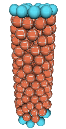
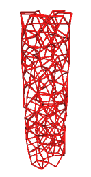
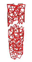
(a) (b) (c)

Figure 1: (a) A typical test setup with aspect ratio $s\simeq 3$ and $N=200$. The smooth, blue particles are the driving particles, the striped brown ones are the bulk particles. (b) The contact network of the same system. (c) The broken contact network after strain $\varepsilon=0.00017$. Note, that particle displacement would not be visible.

The tests were done in absence of gravity and without the compressing plates. There are fewer contacts from the bulk to a plate than to a layer of particles, thus if plates were used for driving it would be expected that the contacts between a plate and the touching particles would fail first. So we chose the last layers of particles (the ones that are closer than $1.1$ particle radius to the compressing plate) to move as a rigid body and drive the system. This allows the failure zone to be everywhere in the sample. A typical setup and test result is shown on Fig. 1.

Two different driving methods were used: (i) the driving layer had infinite mass, (ii) the driving layer had infinite mass only in the driving direction but finite in the perpendicular directions. Since no significant difference was observed, the results reported in this paper are shown with driving particles of infinite mass. The driving velocity was always kept low enough as to avoid kinetic effects.

After the preparation the sample was tested. At the beginning of the tests all existing (i.e. force transmitting) contacts were “glued”, all subsequent contacts (including broken ones at later times) were handled with the standard Hooke contact law including static friction. The simulation was run long enough such that the upper and lower part are completely separated as shown on Fig. 1(c).

The different tests were realized by giving the driving particles on both sides of the sample initially a velocity (or angular velocity) in the required direction but with opposing sign.

3.2 Parameters

In order to interpret the results of numerical simulations we have to take a closer look at the dimensions of the parameters. Due to the quasi static nature of the tests (up to the failure point) and the absence of gravity, quantities like time and mass are unimportant, instead force and distance units determine the scales of the numerical results.

Two parameters of dimension distance enter: the average particle diameter $\bar{d}$ and the contact glue diameter $2a$. Since in all simulations the ratio $a{=}0.1\bar{d}$ was used, $\bar{d}$ is taken as the unit of length.

The stress or force scale is set by the stress threshold $\sigma_{*}$ (cf. (24)) and $F_{*}=\pi a^{2}\sigma_{*}$, respectively. Due to technical reasons, 17 times the latter was chosen as unit of force.

Thus, from now on all quantities will be given in this natural units ($\bar{d}$ for length and $17F_{*}$ for force).

The normal contact stiffness $k_{n}$ (the tangential one is set to $k_{t}{\equiv}k_{n}/2$, corresponding to the limit $\nu=0$, cf. (14)) relates force and length and must fulfill $k_{n}\gg 1$ to assure the brittle limit. This can also be expressed as the failure strain scale

$$\varepsilon_{*}=\frac{F_{*}}{k_{n}\bar{d}}$$ (34)

being very small.

The preparation was done with the aim to achieve a sample as homogeneous and isotropic as possible. For such a random configuration, the macroscopic Young’s modulus can be calculated analytically micromacro2 ; micromacro1 from the stiffness parameters of the contacts:

$$E=\frac{N_{c}\bar{d}}{3V}\frac{\left(2k_{n}+3k_{t}\right)}{4k_{n}+k_{t}}$$ (35)

where $N_{c}$ is the number of contacts and $V$ is the volume of the sample. The latter can be calculated using (33):

$$E=\frac{\bar{z}f(2k_{n}+3k_{t})}{12\bar{d}(4k_{n}+k_{t})},$$ (36)

where $\bar{z}$ is the average coordination number which was measured to be $\bar{z}{\simeq}5.06$ in all cases. This value is less than the isostatic limit for homogeneous packing due to the boundary effects. Using the values $f{=}2.5$ and $k_{t}{=}k_{n}/2$, we get an estimate for the macroscopic Young’s modulus:

$$E=0.81\frac{k_{n}}{\bar{d}}$$ (37)

The macroscopic Poisson ratio can also be expressed as function of the contact stiffness micromacro1 ; micromacro2 :

$$\nu=\frac{k_{n}-k_{t}}{4k_{n}+k_{t}}=0.11$$ (38)

The actual simulation parameters (in natural units) chosen for the current study were taken to allow reliable and fast simulation of the tests and yet fulfill the requirements above:

$$\bar{d} =1 a =0.1$$ (39)

$$k_{n} =1256 k_{t} =k_{n}/2$$ (40)

$$\sigma^{*} =1.88$$ (41)

From those we can calculate the macroscopic Young’s modulus (36) and Poisson ratio (38) as well as the limit strain (34):

$$E=1017\quad,\quad\nu=0.11\quad,\quad\varepsilon_{*}=9.4\times 10^{-5}$$ (42)

4 Yield tests

4.1 Poisson ratio

The easiest quantity that we can measure in our simulations is the Poisson ratio. In pull experiments we recorded the displacement of the driving particles in the $z$ direction and the radius of the sample at $z{=}H/2$. The latter was done by averaging the outer radius over all surface particles that have at least two contacts (remove rattling, dangling particles). Since the relative displacement is very small (of the order of $10^{-6}$) we can use the linearized expression for the Poisson ratio:

$$\nu\simeq-\frac{\Delta R}{\Delta H}$$ (43)

We averaged for different samples and system size to get the result:

$$\nu=0.108\pm 0.01$$ (44)

This value is in perfect agreement with the prediction of (42).

4.2 Stress/strain behavior

Three different tests were done: pull, shear and twist. In the tests the driving was realized by giving the driving particles a constant (angular) velocity. The net force (torque), the number of intact contacts, the deformation of the sample was recorded as function of the displacement of the driving particles.

The stress/strain evolution of the samples in the homogeneous and isotropic case are described by three parameters: Young’s modulus $E$, Poisson ratio $\nu$ and maximal strain $\varepsilon^{*}$. So the evolution of all test should be described by one single curve. Thus the measured displacement and force (torque) data has to be converted to a stress/strain relation.

It is more informative if this conversion is done with the dimensionless quantities of the aspect ratio $s$ and the number of particles $N$ since it allows immediately the scaling of different tests in a transparent manner.

In general the stress and the strain are not homogeneous, so we focus on their two important characteristics: the maximum and the average. The maximum stress governs the point where the first contact breaks, the average value indicates the importance of the inhomogeneities of the stress and we compare it to the maxima of the stress/strain curve.

The pull deformation is homogeneous thus the maximum is the same as the average:

$$\bar{\varepsilon}_{p}=\varepsilon_{p,\mathrm{max}}=\frac{Z}{H}=\frac{(f\pi)^{1/3}Z}{2s^{2/3}N^{1/3}\bar{d}},$$ (45)

where $Z$ is the vertical displacement of the driving particles and $f$ is the volume factor of (33). The stress can be taken directly from section 2.1:

$$\bar{\sigma}_{p}=\sigma_{p,\mathrm{max}}=\frac{F_{z}}{\pi R^{2}}=\left(\frac{fs}{\sqrt{\pi}N}\right)^{2/3}\frac{F_{z}}{\bar{d}^{2}}$$ (46)

The twist deformation has a radius dependence, but apart from this is very similar to the previous case.

$$\varepsilon_{t,\mathrm{max}} =\frac{R\alpha}{H}=\frac{\alpha}{2s}$$ (47)

$$\bar{\varepsilon}_{t} =2\varepsilon_{t,\mathrm{max}}/3,$$ (48)

where $\alpha$ is the angle covered by the driving layer. The form of the stress again is identical to the microscopic one in 2.1:

$$\sigma_{t,\mathrm{max}} =\frac{4T(1+\nu)}{\pi R^{3}}=\frac{4f(1+\nu)s}{N}\frac{T}{\bar{d}^{3}}$$ (49)

$$\bar{\sigma}_{t} =2\sigma_{t,\mathrm{max}}/3$$ (50)

The shear deformation is a bit more involved than the previous ones, since its behavior is fundamentally different whether the aspect ratio is large or small compared to unity (with a crossover in between). The short cylinder limit was covered in Sec. 2.1. The long cylinder limit is more complicated, but consists of a combination of bending and shearingSokolnikoff_book as well. We define here the strain as the most straightforward interpolation of the two cases that recovers the short cylinder result for $s\to 0$ and the long cylinder form in the limit $s\to\infty$:

$$\varepsilon_{s,\mathrm{max}} =\frac{X}{H(1+\frac{H}{8R})}=\frac{(f\pi)^{1/3}X}{2s^{2/3}N^{1/3}\bar{d}(1+s/4)}$$ (51)

$$\bar{\varepsilon}_{s} =\frac{4\varepsilon_{t,\mathrm{max}}}{3\pi},$$ (52)

Applying Hooke’s law to the whole strain field yields the interpolating stress

$$\sigma_{s,\mathrm{max}} =\frac{F_{x}\left(2\nu+2+\frac{H^{2}}{3R^{2}}\right)}{\pi R^{2}(1+\frac{H}{8R})}=$$ (53)

$$=\left(\frac{fs}{\sqrt{\pi}N}\right)^{2/3}\frac{\left(2\nu+2+\frac{4s^{2}}{3}\right)}{(1+s/4)}\frac{F_{x}}{\bar{d}^{2}}$$ (54)

$$\bar{\sigma}_{s} =\frac{4\sigma_{s,\mathrm{max}}}{3\pi}\quad.$$ (55)

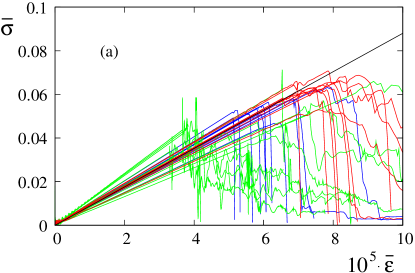
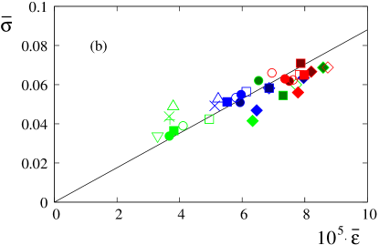
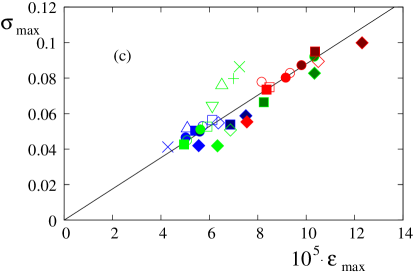
Figure 2: Color online. (a) Stress strain evolution (b) The maximum of the average stress, (c) End of elasticity (first broken contact) in the stress/strain plain. Colors represent experiment type pull: blue, shear: green, twist: red. Symbol fill intensity indicates system size $N$: $200$: half, $2000$: empty, $10000$: full. Symbol types show aspect ratio $s$: 1: $\diamond$, 2: $\square$, 3: $\bigcirc$, 5: $\bigtriangleup$, 7: $\bigtriangledown$, 8: $+$, 10: $\times$

Figure 2 (a) shows the average stress/strain curves for different experiments, system size, sample length. The measured Young’s modulus varies around a mean value $E{\simeq}880$, which is 15% less than the theoretical value of (37). There is a slight scatter of the linear slope of different systems but in spite of the moderate system size still one can observe a convincing data collapse with different system size, aspect ratio and test type.

In Fig. 2 (b) the maxima of the average stress/strain curves are shown as function of the average strain. It is evident that the elastic behavior is very close to the Hooke’s law and can be described by a single Young’s modulus. The average macroscopic stress and strain are always smaller than the scale (42), as must be expected due to spatial disorder.

The maximal stress/strain values at the moment of the first broken contact are plotted in Fig. 2 (c). The values are scattered around $\varepsilon_{*}$ of (42). We note two important features: (i) points which are above $\varepsilon_{*}$ are mainly for system size $N{=}200$ and for shear and twist tests. This is the result of the inhomogeneities of our system. Due to the preparation procedure the volume fraction at the lateral surface of the cylinder is larger than in the bulk. This was tested by repeating a few tests with a sample cut out from a bigger one, and this feature disappeared. (ii) Maximal stresses for long cylinders in shear tests are somewhat larger than expected, these are the result of the same skin effect during the bending of the sample.

4.3 Yield criteria

In the simulations we used all three criterions introduced in Sec. 2.2. We performed test using exactly the same initial configuration with the different break criterions. Fig. 3 shows the summary of the results.

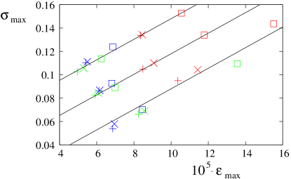
Figure 3: The stress and the strain points where the first contact was broken. Colors represent experiment type pull: blue, shear: green, twist: red. Symbols indicate the different break criterions: Full $+$, Simplified: $\times$, Decoupled $\square$. System size $N{=}200$, 2000, $10000$, are from bottom to top respectively with artificial shifting of $0.3$. The aspect ratio was chosen to be $s{=}2$

The results show hardly any difference between the two coupled criterions (simplified (31) and full (25), however the decoupled criterion allows the system to evolve without failure beyond the point where the others already broke.

It is remarkable that the simple coupling of the different deformation modes leads to indistinguishable failure points for large systems. For small systems the only difference is in the twist deformation.

The elapsed time during simulations was also measured. We observed no measurable difference in simulation duration of tests with decoupled and simplified criterions. Simulations with the full criterion on average require 55% more time independently of system size. This advocates the use of the simplified criterion if computational time is critical but this overhead is relatively small in spite of the numerical maximization of (25) which is in general affordable if precision is required.

4.4 Failure process

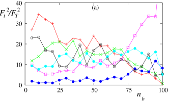
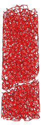
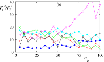
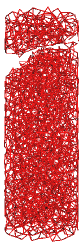
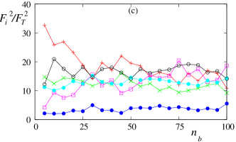
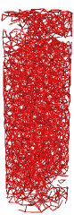
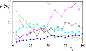
Figure 4: Color online. Average (sample and time) deformation forces in just broken contact bridges scaled by the maximal force versus $\tilde{N}_{b}$. (a) Pull test with $s{=}3$ (b) Twist test with $s{=}3$ (c) Shear test with $s{=}3$, (d) Shear test with $s{=}0.5$. The symbols represent the following deformation component: tensile: $+$, shear: $\times$, tilt: $\bullet$, torsion: $\square$, tilt+tensile: $\blacksquare$, torsion+shear: $\bigcirc$. On the right hand side of the plots a typical example of force network plot is shown for the given system after the test.

In this section we study the process of the failure in the tests. Our simulations allow the study of each individual broken contact. The question we want to answer here is: Which is the deformation type that is the most relevant for a give test.

We identify 6 different deformation types which are the core of the simplified break criterion (31):

$$\mathrm{tensile:} F_{z}^{2}/4$$ (56)

$$\mathrm{shear:} F_{x}^{2}+F_{y}^{2}$$ (57)

$$\mathrm{tilt:} 4T^{2}_{x}/a^{2}$$ (58)

$$\mathrm{torsion:} 4T^{2}_{z}/a^{2}$$ (59)

$$\mathrm{tilt+tensile} 2|F_{z}t_{x}-2F_{x}T_{z}|/a$$ (60)

$$\mathrm{torsion+shear} 4|F_{y}T_{z}|/a,$$ (61)

In order to study the relevance of the above deformation types, the following procedure was used: At the moment of a contact break, the above quantities are recorded.

Since we have a random packing, the values show huge variations from contact to contact. An average is necessary to be able to observe the different trends. We averaged the recorded limit forces for each successive 5% of broken contacts. So if $N_{b}(t)$ is the number of broken contacts at time $t$ then the $x$ axes shows $n_{b}{=}N_{b}(t)/N_{b}(T)$, with $T$ being the time at the end of the experiment. This representation allows us to average also for different sample realizations (5-10) so that early and late stages of failure can be identified, as shown in Fig. 4.

The beginning of the pull test [Fig. 4 (a)] is marked by contacts strained in the tensile direction. This dominance is clear for the first 25% broken contacts but remains the most important up to 60% broken contacts. The end stage (after 75% of the contacts were broken), is surprisingly characterized by contacts breaking due to torsion. Our view is that this is due to breaking of small chains, namely a single particle having two contacts one to each side of the sample. In general, since all “strong” contacts are already broken, its two contacts are loaded mainly with a combination of torsion and tilting. A remarkable feature is that tilting gets stabilized by shear and tensile forces, while torsion is not. This can be seen by the fact that tilting+tensile deformation is almost the second most important loading at late stages. Since we have used a rather narrow contact diameter $a{=}0.1\bar{d}$, contacts break easily under torsional load.

Twist tests [Fig. 4 (b)] show a surprisingly similar picture to pull experiment, except that at early stages it is the shear deformation which dominates. The late stage is also dominated by torsional deformation.

The behavior of shear tests are fundamentally different depending on the aspect ratio. If the aspect ratio is small [$s<1$, Fig. 4 (d)] the overall behavior is similar to the twist deformation: shear dominates at early stages and torsion at late ones.

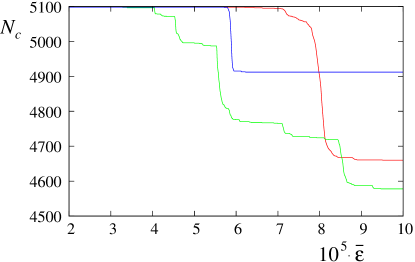
Figure 5: (Color online) The number of contacts as function of the average strain for $s{=}3$ and $N{=}2000$, for the tests: pull: blue, shear: green, twist: red

It is common to all of the above cases that the stress/strain behavior of the sample is determined by the contacts that broke in the early stages, moreover the whole fracture is realized very fast in a cascade like manner as shown on Fig. 5, as to be expected in the brittle limit.

The only test where a different scenario can be observed is the shear test with long cylinders [Fig. 4 (c)]. At early stages the tensile deformation dominates. This is due to the bending of the sample. The force network shows that the contacts start to break at two points simultaneously. These points are the ones where the material is stretched the most (right at the moving “front” of the driving layer). The stress is very localized so despite the damage the sample has still a significant resistance which is manifested by the long oscillating tail of the stress/strain curve [Fig. 2 (a)] and the slow step-wise decreasing of the number of contacts.

5 Conclusion

In this paper we introduced a new model for DEM simulations with breakable cemented contacts. Contacts were considered as small, flat, elastic cylinders which keep the particles in contact until the shear stress in the cementing cylinder reaches a maximal value conforming to the Tresca criterion of failure. This allowed for deriving the elastic and the failure behavior of the contact on a common basis. In the limit of very flat cylinders, the stiffness matrix (14) gets decoupled, justifying this common a priori modelling Ansatz.

The problem of finding the maximal shear stress in an arbitrarily loaded cylinder turned out to possess analytic solutions too complicated for practical purposes (but is numerically well accessible). Therefore we considered two approximations: The decoupled criterion coincides with the exact maximization only for single loading modes, while the simplified criterion agrees with the latter in more general situations, due to taking into account load combinations. We showed that decoupling the loads leads to a rather large error of 25%, whereas the simplified criterion agreed with the full one within statistical errors. This applies to our tests, but in the case of the full criterion turning out to be necessary in other situations, the found overhead of 55% for the numerical maximization is affordable.

As a benchmark, we have done pull, shear and torsion tests with cylindrical specimens created from glued particles. These exhibited, up to the failure point, an elastic behavior with the same Young’s modulus for all experiments and test parameters. This enabled us to collapse all different test results onto one single curve. The deviations of the theoretical prediction for the specimens’ elastic properties were below 15%.

During the tests we payed special attention to the dominant loading of the contacts that are about to break. We found that the first half of broken contacts in pull tests mostly break due to tensile stress, in twist tests due to shear stress, and in shear tests of very short samples due to shear stress as well. Long samples behave differently in shear tests, though, due to bending the dominating load gets tensile instead of shear. Finally, the late stages of the failure is mainly characterized by contacts breaking under torsional load due to break up of twisted weak chains connecting the almost separated parts.

For the sake of a clearer study of this relative importance of the loading types and the different failure criteria, we used a constant diameter of the contact cylinders. In future works, the stochastic nature of the geometry and strength of the contact, possibly obeying a wide distributionBirkenfeld , will be taken into account.

6 Acknowledgements

The authors acknowledge the financial support from the German Research Foundation (DFG grant BR 3729/1) and thank Sandia National Laboratories (of the US Department of Energy) for putting LAMMPS under the GNU Public License.

References

- (1) Antonyuk, S., Khanal, M., Tomas, J., Heinrich, S., Mörl, L.: Impact breakage of spherical granules: Experimental study and dem simulation. Chemical Engineering and Processing: Process Intensification 45(10), 838–856 (2006)
- (2) Borghi, R., Bonelli, S.: Towards a constitutive law for the unsteady contact stress in granular media. Continuum Mech. Thermodyn. 19, 329–345 (2007)
- (3) Cundall, P., Strack, O.: A discrete numerical model for granular assemblies. Geotechnique 29, 47–65 (1979)
- (4) Delenne, J.Y., Youssoufi, M.S.E., Cherblanc, F.: Mechanical behaviour and failure of cohesive granular materials. Int. J. Numer. Anal. Meth. Geomech. 28, 1577–1594 (2004)
- (5) Herrmann, H.J., Hovi, J.P., Luding, S. (eds.): The Physics of Dry Granular Media, vol. 350. Kluwer, Dordrecht (1998)
- (6) Kirsch, R., Brendel, L., Török, J., Bröckel, U.: Measuring tensile, shear and torsional strength of solid bridges between particles in the millimeter regime. Submitted to this journal
- (7) Kuhl, E., d’Addetta, G.A., Herrmann, H.J., Ramm, E.: A comparison of discrete granular material models with continuous microplane formulations. Granular Matter 2, 113–122 (2000)
- (8) Luding, S.: Collisions & contacts between two particles. In: Herrmann et al. PhysDryGran_97 , pp. 285–304
- (9) Mitarai, N., Nori, F.: Wet granular materials. Advances in Physics 55(1), 1–45 (2006)
- (10) Plimpton, S.: Fast parallel algorithms for short-range molecular dynamics. J. Comp. Phys. 117, 1–19 (1995)
- (11) Pöschel, T., Luding, S. (eds.): Lecture Notes in Physics: Granular Gases, vol. 564. Springer (2001)
- (12) Roux, S.: Quasi-static contacts. In: Herrmann et al. PhysDryGran_97 , pp. 267–284
- (13) Sokolnikoff, I.S.: Mathematical Theory of Elasticity. Krieger, Malabar, Florida (1983)
- (14) Tresca, H.: Mémoire sur l’écoulement des corps solides soumis à de fortes pressions. C.R. Acad. Sci. Paris 59, 754 (1864)
- (15) Wang, Y., Alonso-Marroquin, F.: A finite deformation method for discrete modeling: particle rotation and parameter calibration. Granular Matter 11, 331–343 (2009)