Puzzles with Tachyon in SSFT and Cosmological Applications

Abstract

This work is my contribution to the proceedings of the conference “SFT2010 – the Third International Conference on String Field Theory and Related Topics”. We discuss properties of nonlocal tachyons and nonlocal SFT inspired cosmology.

1 Introduction

In this talk I would like to discuss time dependent solutions for the tachyon field in cubic (super)string field theories. The key new property of the tachyon field is that it satisfies a nonlocal equation.

The plan of this talk is the following:

• Yukawa field and string field

• Nonlocality in SFT and SFT inspired models

• Applications of SFT nonlocality to cosmology

• Mathematical questions around nonlocal cosmology

1.1 Yukawa field and string field

We are at the Yukawa Institute and it is worth reminding that in 1949 Yukawa to remove divergences in QFT had proposed a nonlocal model, which is free from the restriction that field quantities are always point like functions in the ordinary space [1]. The Yukawa field $U(x,r)$ depends on the spacetime coordinates $x$ and an extra vector $r$ and is the subject of the restriction

$$(r_{\mu}r^{\mu}-\lambda^{2})U(x,r)=0,$$ (1)

as well as a solution to the Klein-Gordon equation. The main motivation to deal with nonlocal models in old days was the elimination of divergences, see also [2, 3, 4, 5]. There is a similarity between the expansion

$$U(x,r)=\phi(x)+A_{\mu}(x)r^{\mu}+B_{\mu\nu}(x)r^{\mu}r^{\nu}+...$$ (2)

and the SFT expansion

$$\Phi[x(\sigma)]=\phi(x)+A_{\mu}(x)\alpha^{\mu}_{-1}+...\,.$$ (3)

One can say that the Yukawa field $U(x,r)$ is a prototype of the modern string field $\Phi[x(\sigma)]$.

1.2 Nonlocality in strings

Elimination of divergences is also one of the main goals of string theories. Generally spiking, nonlocality in string theories is related with extended character of the Nambu-Goto string and is related with the string parameter $\alpha^{\prime}$.

1.3 Nonlocality in String Field Theory

1.3.1 In fundamental setting

Nonlocality is a characteristic feature of noncommutative geometry. The covariant Witten string field theory (SFT)[6] is an example of noncommutative geometry. The light-cone Kaku-Kikkawa SFT [7] and covariant light-cone-like HIKKO (Hata-Itoh-Kugo-Kunitomo-Ogawa) [8] SFT have nonlocal features. The same concerns the cubic fermionic AMZ-PTY (Aref’eva, Medvedev, Zubarev and Preitschopf, Thorn, Yost) SFT [9] as well as the fermionic nonpolynomial Berkovits SFT [10]. Nonlocality in SFT is a subject of several discussions [11, 12, 13].

1.3.2 In practical setting

By practices I mean cosmological applications. In cosmology we study time-dependent solutions in a nontrivial cosmological metric,

$$ds^{2}=-dt^{2}+a^{2}(t)dx^{2}.$$ (4)

We do not have in our disposal SFT in a nontrivial cosmological background. We start from a discussion of time-dependent solutions in the flat case. The equation of motion for the cubic SFT has a simple form

$$Q\Phi+\Phi\star\Phi=0$$ (5)

Because the BRST operator $Q$ has nontrivial cohomologies, the zero-curvature equation (5) has nontrivial solutions. An active search for Higgs-type solutions of (5), i.e. solutions for which all component fields are constant, began in 1999. This activity was primarily associated with the Sen conjectures (see [14]). There were many attempts to find numerical solutions of (5) and verify the Sen conjectures in the framework of the level-truncation method. The impulse for a new development came from a remarkable Schnabl’s paper [15]. In this paper explicit solutions of Eq. (5) have been found for the boson string (see refs.[16, 17] for simplifications of this solution). In subsequent papers [18, 19, 20, 21, 22, 23] solutions have been found for the NS fermionic string. In the bosonic case level-truncated vacuum solutions are rather closed to the exact one. In fermionic case the analytical solution [19] starts from the level-truncated solution [24]. There are also exotic universal solutions [25].

There were several attempts to find time depending level-truncated solutions [26, 29, 27, 28, 30] as well as exact solutions. There is a hope that study of marginal deformed theory would help to find exact rolling solutions [31, 32, 33, 34, 35, 36, 37]. However finding analytical time depending solutions suitable for cosmological applications is still an open problem in SFT. By this reason and motivated that leading level-truncated versions of SFT actions reproduce qualitatively known exact results, we discuss cosmological applications within a level-truncated model [38].

2 Nonlocal Cosmology from String Field Theory

2.1 Model

Our nonlocal cosmological model is given by the following action [38]

$$S=\int d^{4}x\sqrt{-g}\left\{\frac{R}{2\kappa^{2}}+\frac{1}{\lambda_{4}^{2}}\left(-\frac{\xi^{2}\alpha^{\prime}}{2}g^{\mu\nu}\partial_{\mu}\phi(x)\partial_{\nu}\phi(x)+\frac{1}{2}\phi^{2}(x)-\frac{1}{4}\Phi^{4}(x)-T^{\prime}\right)\right\}$$ (6)

Here $g_{\mu\nu}$ is the four-dimensional metric, $\kappa$ is the gravitational constant and $\lambda_{4}$ is the scalar field coupling constant. In this SFT nonlocal model our Universe is considered as a D3 non-BPS brane embedded in the 10-dimensional space-time. Due to this embedding we have

$$\frac{1}{\lambda_{4}^{2}}=\frac{v_{6}M_{s}^{4}}{g_{o}}\left(\frac{M_{s}}{M_{c}}\right)^{6},$$ (7)

$g_{o}$ is the open string dimensionless coupling constant, $M_{s}$ is the string scale $M_{s}=1/\sqrt{\alpha^{\prime}}$ and $M_{c}$ is a scale of the compactification, $v_{6}$ is a number related with a volume of the 6-dimensional compact space. The role of the dark energy plays the Neveu-Schwarz (NS) string tachyon leaving in the GSO$-$ sector. The tachyon action is dictated by the cubic fermionic SFT [24] and it is nonlocal due to string effects. The form of the nonlocal interaction defined by the cubic fermionic SFT (CFSFT) [24] is in fact a more complicated as compare with $\Phi^{4}$, where $\Phi$ is related with the tachyon field $\phi$ by the following relation

$$\Phi=e^{\frac{\alpha^{\prime}}{8}\Box_{g}}\phi,~{}~{}~{}{\mbox{where}}~{}~{}~{}\Box_{g}=\frac{1}{\sqrt{-g}}\partial_{\mu}\sqrt{-g}g^{\mu\nu}\partial_{\nu}.$$ (8)

But, by analogy with the flat case [27, 28] we believe that the approximation accepted in (6) reflects essential physical properties of the model. $\xi^{2}\approx 0.9556$ is a constant defined by the CFSFT.

The potential has perturbative and nonperturbative minima. A transition from a perturbative vacuum to a non-perturbative one is interpreted as D-brane decay. In the flat background the D-brane tension $T$ is equal to 1/4, and this value is compensated by the minimal value of the tachyon potential (Sen’s conjecture), so that the total vacuum energy is zero. This compensation means that the cosmological constant is zero,

$$\Lambda\equiv T+V_{0}=0.$$ (9)

In (6) we postulate a minimal form of the tachyon interaction with gravity. The total energy of the system in the true non-perturbative vacuum we interpret as the cosmological constant,

$$\Lambda^{\prime}\equiv T^{\prime}+V_{0}.$$ (10)

It has been conjectured [39] that an existence of a rolling solution describing a smooth transition to the true vacuum in a given cosmological background does define the value of the cosmological constant. We cannot prove this conjecture but arguments to its favor were given using the local approximation [40]. A recent breakthrough in solving numerically the full nonlinear and nonlocal system of equations [41] also supports this conjecture.

Under some conditions our nonlocal model admits a local approximation and displays a phantom behaviour [28]. Note that unlike phenomenological phantom models here the phantom appears in an effective theory. Since SFT is a consistent theory this approach does not suffer from usual problems which are inevitable for phenomenological phantom models.

2.2 Problems

The questions that we address in nonlocal cosmology are concerned two different epochs of the Universe evolution, namely physics just after Big Bang and the modern evolution.

• About the modern evolution epoch we would like to know

  • why now the cosmological constant is so small;

  • can we construct a physically acceptable dynamical dark energy (DE) model with $w<-1$

  • can we get a periodic crossing the $w=-1$ barrier

  It is natural to rise these questions since present cosmological observations do not exclude an evolving DE and according to recent data we have for the state parameter $w=-1.04\pm 0.06.$ Local DE models with the state parameter $w<-1$ violate the null energy condition (NEC).

• As to the early time evolution we would like to know

  • can we construct an inflation nonlocal model with a large non-Gausianity;

  • can we estimate influence of presence of nonlocal matter on primordial black holes formation

  About applications of nonlocal SFT models to the DE problem see [38, 39, 40, 42, 41], to inflation see [43, 44, 45, 46, 47] and to cosmological singularity see refs. in [48].

2.3 How we study the model and what we get

In the spatially flat FRW metric the dynamics in the model (6) is described by a system of two nonlinear nonlocal equations [38] for the tachyon field and the Hubble parameter $H(t)=\dot{a}/a$

$$\left(\xi^{2}{\cal D}+1\right)e^{-\frac{1}{4}{\cal D}}\Phi = \Phi^{3},$$ (11)

$$3H^{2} = \frac{\kappa^{2}}{\lambda_{4}^{2}}\left(\frac{\xi^{2}}{2}\partial_{t}\phi^{2}-\frac{1}{2}\phi^{2}+\frac{1}{4}\Phi^{4}+{\cal E}_{1}+{\cal E}_{2}+T^{\prime}\right),$$ (12)

where ${\cal D}=-\partial_{t}^{2}-3H(t)\partial_{t},\,\,\,\,\,H=\partial_{t}a/a$ and

$${\cal E}_{1} = -\frac{1}{8}\int_{0}^{1}ds\left((\xi^{2}{\cal D}+1)\,\,\,e^{\frac{s-2}{8}{\cal D}}\Phi\,\right)\cdot\left({\cal D}\,\,e^{-\frac{1}{8}s{\cal D}}\Phi\right),$$ (13)

$${\cal E}_{2} = -\frac{1}{8}\int_{0}^{1}ds\left(\partial_{t}(\xi^{2}{\cal D}+1)\,e^{\frac{s-2}{8}{\cal D}}\Phi\right)\cdot\left(\partial_{t}e^{-\frac{1}{8}s{\cal D}}\Phi\right).$$ (14)

The nonlocal energy ${\cal E}_{1}$ plays the role of an extra potential term and ${\cal E}_{2}$ the role of the kinetic term. Note that here we use a dimensionless time $t\to t\sqrt{\alpha^{\prime}}$.

Equations (11) and (12) form a rather complicated system of nonlinear nonlocal equations for functions $\Phi$ and $H(t)$ because of the presence of an infinite number of derivatives and a non-flat metric. Before to discuss the methods of study this model let us mention the known methods of study equation (11) in the flat background, $H=0$,

$$\left(-\xi^{2}\partial_{t}^{2}+1\right)e^{\frac{1}{4}\partial_{t}^{2}}\Phi(t)=\Phi(t)^{3}.$$ (15)

$\xi=0$ corresponds to p-adic string (see [49]and refs therein). Equation (12) in the flat case describes the energy conservation [28]. A boundary problem $\Phi(\pm\infty)=\pm 1$ for (15) has been studied using different methods. A numerical method [27] is based on an integral representation of (15). The integral representation has also been used to prove existence theorems [50, 51, 52] and is also related with a diffusion equation method [53]. This method uses an auxiliary function of two variables $\Psi(\lambda,t)$ satisfying the diffusion equation

$$(\partial_{\lambda}-\partial_{t}^{2})\Psi(t,\lambda)=0,$$ (16)

$\Phi(t)=\Psi(t,0)$ and Eq.(15) becomes the boundary condition

$$\left(-\xi^{2}\partial_{t}^{2}+1\right)\Psi(t,\frac{1}{4})=\Psi(t,0)^{3}$$ (17)

The following characteristic properties of (15) have been obtained. First is an existence of a critical point $\xi^{2}_{\text{cr}}\approx 1.38$ such that for $\xi^{2}<\xi^{2}_{\text{cr}}$ eq. (15) has a rolling solution [27] interpolating between $\pm 1$. Second is an existence of a dominance of an extra nonlocal kinetic term ${\cal E}_{2}$ over the local kinetic one [28] and as a result, an appearance of a phantom behavior providing $w<-1$.

There is also a method of decomposition on local fields [54, 42, 55, 56]. This method works well for linear equations and has been used to study solutions to (15) near vacuum $\pm 1$. It is very interesting to find approximate models admitting explicit solutions and having above mentioned properties. They could contain two or more components local fields. Let us also mentioned almost exact solutions methods [57, 48].

An investigation of non-flat eqs. (11) and (12) is essentially more complicated. A numerical study has been performed in [41]. A decomposition on local fields have been used in [40, 48, 59, 55]. A simplest one phantom mode approximation with a special six-order potential [40] has the solution

$$\phi(t)=\tanh(t)$$ (18)

and gives $\Lambda\equiv 1/4+V_{0}^{\prime}=1/m^{4}_{p}$, where $m^{4}_{p}$ is the reduced Planck mass

$$m^{2}_{p}\sim\frac{M_{s}^{2}}{M_{p}^{2}}(\frac{M_{s}}{M_{c}})^{6}.$$ (19)

The difference $V_{0}^{\prime}-1/4$ is assumed coming from nontrivial background effects. Assuming also that $M_{c}\sim M_{p}$ and $M_{s}\sim 10^{-6.6}M_{p}$ we get a possibility to explain the small value of the Hubble parameter in the real time $H_{0}\sim M_{s}/m_{p}^{2}$, namely

$$H_{0}\sim 10^{-60}M_{p}.$$

3 Generalization of SFT cosmology

3.1 Models

A generalization of the nonlocal SFT cosmological model (6) has the form

$$S=\int d^{4}x\sqrt{-g}\left\{\frac{R}{2\kappa^{2}}+\frac{1}{g^{2}_{o}}\left(\frac{1}{2}\Phi(x)F(\Box_{g})\Phi(x)-V(\Phi)-T^{\prime}\right)\right\},$$ (20)

where $F(z)$ in a neighborhood of the point $z=0$ is an analytic function and

$$F(\Box_{g})=\sum\limits_{n=0}^{\infty}f_{n}\Box_{g}^{\;n}.$$ (21)

Such type of models have been considered in [54, 55, 42]. A special interest presents the case of $\zeta(\Box)$, where $\zeta(s)$ is the famous Riemann zeta-function [60]. One of the reasons to consider this case is that the Riemann zeta-function is universal in the sense that any analytic function can be approximated by the shifts of the Riemann zeta-function.

Modified gravity cosmological models have been proposed in the hope of finding to solutions to the open problems of the standard cosmological model. There are a lot of ways to deviate from the Einstein gravity. Different modifications of gravity are considering nowadays in the literature. A simple nonlocal gravity has the form

$$S_{3}=\int d^{4}x\sqrt{-g}\left\{\frac{1}{{16\pi G_{N}}}R\left(1+{\cal F}(L^{2}\Box)R\right)+{\cal L}_{\rm matter}\right\},$$ (22)

where ${\cal F}(z)$ is an analytic function at the point $z=0$.

3.2 Mathematical questions around nonlocal cosmology

3.2.1 Nonlocal kinetic operator as a pseudo-differential operator

Let us consider the nonlocal Klein–Gordon equation

$$F(\Box)\phi=0,$$ (23)

If $F(z)$ is a polynomial, then (23) is a partial differential equation, otherwise (23) is a pseudo-differential equation and we have to pay a special attention to a definition of operator $F(\Box)$. In the flat space-time, $(t,x_{i})\in M^{4}$, $\Box={}-\partial^{2}_{t}+\partial_{x_{i}}\partial_{x_{i}}$ and $F(\Box)$ is defined via the Fourier transform [5, 26, 50, 54]

$$F(\Box)\phi(x)=\frac{1}{(2\pi)^{4}}\int\,F(-k^{2})\tilde{\phi}(k)e^{-ixk}d^{4}k,\,\,\,k^{2}=-k_{0}^{2}+k^{2}_{i},\qquad i=1,2,3.$$ (24)

where $\tilde{\phi}(k)$ is a Fourier transform of a function $\phi(x)$, $\tilde{\phi}(k)=\int\phi(x)e^{ikx}d^{4}x$.

In cosmology we usually deal with a positive time variable, $t>0$, and it is more suitable to use the Laplace transform of the time variable and the Fourier transform at space variables [61], $\tilde{\varphi}(s,\vec{k})=\int\limits_{0}^{\infty}dt\int d\vec{x}\varphi(t,\vec{x})e^{-st-i\vec{k}\vec{x}}$. The inverse transform is defined as $\varphi(t,\vec{x})=(2\pi i)^{-4}\,\int\limits_{c-i\infty}^{c+i\infty}d\!s\int d\vec{k}\tilde{\varphi}(s,\vec{k})e^{ts+i\vec{k}\vec{x}}.$

For an analytic function $F(z)$ at $z=0$ we understand the operator $F(\Box)$ as

$$F(\Box)\varphi(t,\vec{x}) = \frac{1}{(2\pi)^{4}i}\int\limits_{c-i\infty}^{c+i\infty}d\!s\int d\vec{k}\,e^{st+i\vec{k}\vec{x}}\left\{F(-s^{2}-\vec{k}^{2})\tilde{\varphi}(s,\vec{k})+r(s,\vec{k})\right\},$$ (25)

$$r(s,\vec{k}) = -\sum_{n=1}^{\infty}\sum_{j=1}^{n}\frac{s^{2n-j}}{n!}\left.\left[\frac{\partial^{n}}{\partial w^{n}}F(-w-\vec{k}^{2})\right]\right|_{w=0}\varphi^{(j-1)}(0,\vec{k}).$$ (26)

This definition is based on the following definition of the time derivatives

$$\partial_{t}^{n}\phi(t)=\frac{1}{2\pi i}\int\limits_{c-i\infty}^{c+i\infty}d\!s\,e^{st}s^{n}\left[\tilde{\phi}(s)-\sum_{j=0}^{n-1}\frac{\partial_{t}^{(j)}\phi(0)}{s^{j+1}}\right]$$ (27)

here $\tilde{\phi}(s)=\int\limits_{0}^{\infty}\phi(t)e^{-st}dt$. Definition (27) has meaning under an assumption that the function ${\ae}_{n}(z)=z^{n}\left[\tilde{\phi}(z)-\sum_{j=0}^{n-1}z^{-j-1}\partial_{t}^{(j)}\phi(0)\right]$ is holomorphic at $\Re\,z\geqslant a$ and satisfies the following condition $|{\ae}_{n}(z)|={\cal O}(|z|^{-1-\alpha}),\,\,\,\mbox{for}\,\,\,|z|\to\infty,\,\,\,\Re\,z\geqslant a\,\,\mbox{and }\,\,a\leqslant c.$ Definition (27) is in agreement with the property

$$\partial_{t}^{m}\partial_{t}^{n}\phi(t)=\partial_{t}^{n+m}\phi(t).$$ (28)

3.2.2 The Weierstrass product and factorization of nonlocal kinetic term

To study the nonlocal Klein–Gordon equation (23) we use [54, 55, 60] (see [5] for early used of the Weierstrass product) the Weierstrass factorization theorem. According to the theorem for any entire function $F$ which is not identically zero, has $m$-order zero at $0$, and has the non-zero counting multiplicity zeroes $\{z_{k}\}$ there exist non-negative integers $p_{1},p_{2},...$ and an entire function $Q_{0}(z)$ such that:

$$F(z)=z^{m}e^{Q_{0}(z)}\prod_{k=1}^{\infty}\left(1-\frac{z}{z_{k}}\right)e^{Q_{k}(z)},\,\,\,\,\,Q_{k}(z)=\sum_{l=1}^{p_{k}}\frac{1}{l}\left(\frac{z}{z_{k}}\right)^{l},$$ (29)

Let us consider equation

$$F(\Box)\phi=-J,\,\,\,\,$$ (30)

for function $F$ that has a finite number of zeros, $F(z)=e^{\mathfrak{f}(z)}\prod\left(z-z_{k}\right),$ and $\mathfrak{f}(z)=\lambda z,\lambda>0$. If we understand the differential operator via its Fourier or Laplace transforms ((24), (25)) then from the factorization of the function $F(z)$ follows the factorization property of the operator $F(\Box)$

$$F(\Box)=e^{\lambda\Box}\prod\left(\Box-z_{k}\right),$$ (31)

and Eq.(30) reduces to two problems

$$1)\,\prod(\Box-z_{k})\psi={}-J\,\,\,\mbox{and}\,\,\,\,\,2)\,e^{\mathfrak{f}(\Box)}\phi=\psi,$$ (32)

A solution to the second equation in (32) depends on the definition of the operator $e^{\mathfrak{f}(\Box)}$ . To solve this equation for $\mathfrak{f}(\Box)=\lambda\Box$ we use the fifth Fock’s parameter method. In this method, one considers the function of two arguments $\Psi(t,\lambda)=e^{\lambda\Box}\phi(t)$ that solves the Fock equation (more precisely, the Euclidean version of this equation, $\lambda=i\tau$, where $\tau$ is the Fock fifth parameter [62]):

$$\partial_{\lambda}\Psi(x,\lambda)=\Box\Psi(x,\lambda)$$ (33)

and the boundary condition

$$\Psi(x,\lambda^{\prime})|_{\lambda^{\prime}=0}=\phi(x).$$ (34)

In this framework the second equation in (32) also can be written as the boundary condition

$$\Psi(x,\lambda^{\prime})|_{\lambda^{\prime}=\lambda}=\psi(x).$$ (35)

Therefore, a solution to the second equation in (32) is reduced to a solution of the boundary problem for the Fock equation . These formal considerations can be put on the mathematical background, in particular, in the case of the space homogeneous configurations.

3.2.3 Exponential equation with quadratic derivatives via Fourier transform.

Let us take $\mathfrak{f}(z)=\lambda z$, $\lambda>0$ and consider

$$e^{\lambda\partial_{t}^{2}}\phi(t)=\psi(t),$$ (36)

$-\infty<t<\infty$, as a linear pseudo-differential equation with the symbol $e^{-\lambda k^{2}}$. We immediately get the integral form of this equation

$${\cal K}[\phi](t,\lambda)=\psi(t)$$ (37)

where ${\cal K}[\phi](t,\lambda)\equiv\frac{1}{\sqrt{4\pi\lambda}}\int\limits_{-\infty}^{\infty}\,\phi(t^{\prime})\,e^{-\frac{(t-t^{\prime})^{2}}{4\lambda}}\,dt^{\prime}.$ Denoting $\Psi(t,\lambda)\equiv e^{\lambda\partial_{t}^{2}}\phi(t)$ we get

$$\partial_{\lambda}\Psi(t,\lambda)=\partial^{2}_{t}\Psi(t,\lambda),\,\,\,\,\,\Psi(t,\lambda)|_{\lambda=0}=\phi(t),\,\,\,\,\,\Psi(t,\lambda^{\prime})|_{\lambda^{\prime}=\lambda}=\psi(t)$$ (38)

             

Figure 1: In the left diagram we illustrate the method of solving the heat equation as a boundary value problem for $-\infty<t<\infty$: the solution (solid line) is defined by the boundary function (a dashed line). The center diagram shows that solution to equation (3.17) is equivalent to solving the inverse diffusion equation, that is the classically ill-posed problem. In the right diagram we show that if the boundary condition (double solid-dashed line) is prepared in a special way, say comes from a boundary conditione at ”early” $\lambda=-a$ (this boundary function is drown by a dashed line), we can solve the boundary problem. In this case the solution (double solid-dotted line) is identical to the solution of the heat equation with the boundary condition denoted by the dashed line.

Assuming that we know $\psi(t)$ we can write

$$\phi(t)=\frac{1}{2\pi}\int e^{\lambda\xi^{2}}\tilde{\psi}(\xi)e^{-i\xi t}d\xi$$ (39)

where $\tilde{\psi}(\xi)$ is the Fourier transform of the source. This integral converges for $\lambda>0$ if the function $\tilde{\psi}(\xi)$ decreases fast enough. In particular, we can assume that there exists $a>0$ such that $\psi(\xi)$ can be presented as $\tilde{\psi}(\xi)=e^{-a\xi^{2}}\tilde{\psi}_{a}(\xi),$ where $|\psi_{a}(\xi)|<C$ for $-\infty<\xi<\infty$, and for $\lambda<a$ the solution to (36) can be presented as

$$\phi(t)={\cal K}[\psi_{a}](t,a-\lambda),$$ (40)

here $\psi_{a}$ is the inverse Fourier transform of $\tilde{\psi}_{a}(\xi)$, see Fig. 1.

For the case $\psi=0$ we get only the trivial solution to equation (36).

3.2.4 Exponential equation with quadratic derivatives on a half axis.

Let us understand the L.H.S. of the equation in (36) as

$$e^{\lambda\partial^{2}_{t}}\varphi(t)\equiv\frac{1}{2\pi i}\int\limits_{c-i\infty}^{c+i\infty}d\!s\,e^{st}\left[e^{\lambda s^{2}}\tilde{\varphi}(s)-\tilde{r}(s,\lambda)\right]$$ (41)

where the residual term $\tilde{r}(s,\lambda)$ is $\tilde{r}(s,\lambda)=\sum_{k=1}^{\infty}\sum_{j=1}^{2k}\frac{\lambda^{k}s^{2k-j}}{k!}d_{j-1},\,\,\,d_{j}=\varphi^{(j)}(0)$. A more general definition with arbitrary constants $d_{j}$ has been discussed in  [61]. This type of definition being applied to an arbitrary function $F(\partial)$ does not guaranty that the factorization form of the operator $F(\partial)$ is the same as the Weierstrass factorization of the function $F(z)$.

Performing summation in the residual term we get the integral representation in $t$-variable

$$r(t,\lambda)={\cal J}_{\frac{1}{2}}[\mathfrak{j}_{0}](t,\lambda)-\frac{1}{2}\,{\cal J}_{\frac{3}{2}}[\mathfrak{j}_{1}](t,\lambda),$$ (42)

where

$${\cal J}_{\frac{1}{2}}[\mathfrak{j}_{0}](t,\lambda) = \frac{1}{2\sqrt{\pi}}\int\limits_{0}^{\lambda}\,d\lambda^{\prime}\frac{e^{-\frac{1}{4}\frac{t^{2}}{(\lambda-\lambda^{\prime})}}}{\sqrt{\lambda-\lambda^{\prime}}}\,\mathfrak{j}_{0}(\lambda^{\prime}),$$ (43)

$${\cal J}_{\frac{3}{2}}[\mathfrak{j}_{0}](t,\lambda) = \frac{t}{2\sqrt{\pi}}\int\limits_{0}^{\lambda}\,d\lambda^{\prime}\frac{e^{-\frac{1}{4}\frac{t^{2}}{(\lambda-\lambda^{\prime})}}}{(\lambda-\lambda^{\prime})^{3/2}}\,\mathfrak{j}_{1}(\lambda^{\prime}),$$ (44)

and $\mathfrak{j}_{0}$ and $\mathfrak{j}_{1}$ are defined via right derivatives of function $\varphi$ at zero

$$\mathfrak{j}_{0}(\lambda)=\sum_{n=0}\frac{\lambda^{n}}{n!}\lim_{y\to+0}\varphi^{(2n+1)}(y),\,\,\,\,\,\,\,\,\,\,\,\mathfrak{j}_{1}(\lambda)=\sum_{n=0}\frac{\lambda^{n}}{n!}\lim_{y\to+0}\varphi^{(2n)}(y)$$

and properly depend on the function $\varphi(t)$ on the half plane $t\geq 0$.

Taking into account that the inverse Laplace transform for $t<0$ is equal to zero we prove that (41) is equivalent to the following representation

$$e^{\lambda\partial^{2}_{t}}\varphi(t)={\cal K}_{+,-}[\varphi](t,\lambda)+{\cal J}_{\frac{3}{2}}[\mathfrak{j}_{1}](t,\lambda)$$ (45)

where ${\cal K}_{+,-}[\phi](t,\lambda)\equiv\int\limits_{0}^{\infty}\frac{e^{-\frac{(t-t^{\prime})^{2}}{4\lambda}}-e^{-\frac{(t+t^{\prime})^{2}}{4\lambda}}}{2\sqrt{\lambda\pi}}\,\phi(t^{\prime})dt^{\prime}.$ The integrant in the second term in the R.H.S. of (45) depends only on even order right derivatives $\lim_{x\to+0}\varphi^{(2n)}(x)$.

Let us remind that the solution to the boundary problem for the heat equation

$$\frac{\partial}{\partial\lambda}\Psi(t,\lambda)=\frac{\partial^{2}}{\partial t^{2}}\Psi(t,\lambda),\,\,\Psi(t,0)=\varphi(t),\,\,\Psi(0,\lambda)=\mu(\lambda)$$ (46)

is given by $\Psi(t,\lambda)={\cal K}_{+,-}[\varphi](t,\lambda)+{\cal J}_{\frac{3}{2}}[\mu]((t,\lambda).$

Representation (45) shows that $\Psi(t,\lambda)=e^{\lambda\partial^{2}_{t}}\varphi(t)$ with the exponential operator that we understand in the sense (41) solves the heat equation with the boundary condition $\Psi(t,0)=\varphi(t)$ and the initial condition $\Psi(0,\lambda)=\mathfrak{j}_{1}(\lambda)$. This initial condition is defined by the boundary function $\varphi$ on the positive half axis.

               

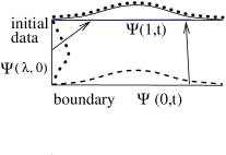
Figure 2: The diagram in the left shows solution of the diffusion equation (double solid-dotted line) with the boundary condition at $\lambda=0$ (dashed line), $0<t<\infty$ and the initial data $\Psi(0,\lambda)=\mu(t)$ (dotted line). The diagrams in the center shows the solution of the diffusion equation with the special initial data (double dotted-dashed line), defined by the boundary function (dashed line). The right diagrams shows solution to Eq.(3.17) (double solid-dashed line) for a special boundary function (thick double solid-dashed line), that is the solution to the diffusion equation for an ”early” boundary condition (dashed line) and the corresponding initial function (double dotted-dashed line).

It is instructive to compare boundary conditions for the heat equation on the axis and on the half axis. Dealing with the heat equation on the axis we fixed the boundary condition at $\lambda=0$ for all $-\infty<t<\infty$, see Fig. 1, meanwhile on the half axis we fixed the boundary condition at $\lambda=0$ only for nonnegative values $0\leq t<\infty$. The initial condition $\mu(\lambda)$ is defined by the boundary function $\Psi(0,t)$.

Eq.(36) for $0\leq t<\infty$, where we understand the exponential $e^{\lambda\partial^{2}_{t}}$ as in (45), can be solved, in particular in the case when the function $\psi(t)$ is defined as a solution of the heat equation in $[-a,\lambda]\times[0,\infty]$ with the given boundary function $\Psi(-a,t)$ and the initial function $\mu(\lambda)=\mathfrak{j}_{1}(\lambda)$ defined by $\Psi(-a,t)$, see the right panel in Fig.2.

3.2.5 Few comments on nonlinear equations

Nonlinear Eq.(15) for $-\infty<t<\infty$, reduces to the integral nonlinear equation

$${\cal K}_{+,-,\xi\,}[\Phi](t,\lambda)=\Phi^{3},$$ (47)

where ${\cal K}_{+,-\,\xi}[\Phi](t,\lambda)=(1+4\xi^{2}\partial_{\lambda}){\cal K}_{+,-\,}[\Phi](t,\lambda)$ and $\lambda=\frac{1}{4}$.

In the case when one deals with $t\geq 0$, the boundary condition due to representation (45) can be presented as an integral equation with the source

$${\cal K}_{+,-,\xi\,}[\Phi](t,\lambda)+{\cal J}_{\xi}[\mathfrak{j}_{1}](t,\lambda)=\Phi^{3}$$ (48)

where ${\cal J}_{\xi}[\mathfrak{j}_{1}](t,\lambda)=(1+4\xi^{2}\partial_{\lambda}){\cal J}[\mathfrak{j}_{1}](t,\lambda)$. It would be interesting to study solutions of the integral equations with sources.

References

- [1] H. Yukawa, Phys.Rev., 76 (1949) 300
- [2] D.I. Blokhintsev, Usp.Fiz.Nauk 61 (1957) 137.
- [3] D.A. Kirzhnits, Usp.Fiz.Nauk 90 (1966) 129.
- [4] V.L. Ginzburg, V.I. Manko, Sov.J.Part.Nucl.7 (1976) 1.
- [5] A. Pais and G.E. Uhlenbeck, Phys. Rev. 79 (1950) 145.
- [6] E. Witten, Nucl. Phys. B, 268 (1986), 253.
- [7] M. Kaku, K. Kikkawa, Phys. Rev. D, 10 (1974) 1110; 10 (1974) 1823.
- [8] H. Hata, K. Itoh, T. Kugo, H. Kunitomo, K. Ogawa, Phys. Lett. B, 172 (1986) 186.
- [9] I.Ya. Aref’eva, P.B. Medvedev, A.P. Zubarev, Phys.Let.B 240 (1990) 356; C.R. Preitschopf, C.B. Thorn, S.A. Yost, Nucl. Phys. B337 (1990) 363; I.Ya. Aref’eva, P.B. Medvedev, A.P. Zubarev, Nucl. Phys. B341 (1990) 464.
-
[10]
N. Berkovits, Nucl. Phys. B, 450 (1995) 90; Erratum:
459 (1996) 439
E. Fuchs, M.Kroyter, JHEP, 10 (2008), 054. - [11] D. A. Eliezer and R. P. Woodard, Nucl. Phys. B 325 (1989) 389.
- [12] H.Hata and H.Oda, Phys.Lett. B394 (1997) 307
- [13] T. Erler and D. Gross, hep-th/0406199
- [14] K. Ohmori, hep-th/0102085; I.Ya. Aref’eva, D.M. Belov, A.A. Giryavets, A.S. Koshelev, P.B. Medvedev, hep-th/0111208; W. Taylor, hep-th/0301094.
- [15] M. Schnabl, Adv. Theor. Math. Phys. 10 (2006) 433
- [16] Y. Okawa, JHEP 0604 (2006) 055.
- [17] T. Erler, M. Schnabl, JHEP 0910 (2009) 066; T. Erler, Theor.Math.Phys.163 (2010) 705
- [18] T. Erler, JHEP, 0801 (2008) 013.
- [19] I. Ya. Aref’eva, R. V. Gorbachev and P. B. Medvedev, Theor.Math.Phys.158 (2009) 3
- [20] I. Ya. Aref’eva, R. V. Gorbachev, D. A. Grigoryev, P. N. Khromov, M. V. Maltsev and P. B. Medvedev, JHEP 0905 (2009) 050
- [21] R. V. Gorbachev, Theor. Math. Phys. 162 (2010) 90
- [22] E. A. Arroyo, arXiv:1004.3030.
- [23] I.Ya. Aref’eva and R.V. Gorbachev, Theor. Math. Phys. 165 (2010) 323
- [24] I. Ya. Aref’eva, A. S. Koshelev, D. M. Belov, P. B. Medvedev, Nucl. Phys. B 638 (2002)3
- [25] T. Erler, arXiv:1009.1865.
- [26] N. Moeller and B. Zwiebach, JHEP 0210 (2002) 034
- [27] Ya.I. Volovich, J. Phys. A36 (2003) 8685.
- [28] I.Ya. Aref’eva, L.V. Joukovskaya, A.S. Koshelev, JHEP 0309 (2003) 012.
- [29] M. Fujita, H. Hata, JHEP 0305 (2003) 043.
- [30] F. Beaujean and N. Moeller, arXiv:0912.1232.
- [31] M. Schnabl, Phys. Lett. B654, 194-199 (2007).
- [32] I.Ellwood, JHEP 0712(2007) 028
- [33] M. Kiermaier, Y. Okawa, L. Rastelli and B. Zwiebach, JHEP 0801 (2008) 028
- [34] O-K. Kwon, Nucl. Phys. B804 (2008) 1.
- [35] T. Kawano, I. Kishimoto and T. Takahashi, Phys. Lett. B 669(2008) 357
- [36] M. Kiermaier, Y. Okawa and P. Soler, arXiv:1009.6185.
- [37] L. Bonora, C. Maccaferri, D. D. Tolla, arXiv:1009.4158.
- [38] I.Ya. Aref’eva, AIP Conf. Proc. 826 (2006) 301.
- [39] I.Ya. Aref’eva, AIP Conf. Proc. 957 (2007) 297.
- [40] I.Ya. Aref’eva, A.S. Koshelev, S.Yu. Vernov, Theor.Math.Phys. 148 (2006) 895
- [41] L. Joukovskaya, Phys. Rev. D 76(2007) 105007 ; L. Joukovskaya, AIP Conf. Proc. 957 (2007) 325; Joukovskaya L.V., JHEP 0902 (2009) 045
- [42] I.Ya. Aref’eva, A.S. Koshelev, JHEP 0702 (2007) 041; A.S. Koshelev, JHEP 0704 (2007) 029; I. Y. Aref’eva and A. S. Koshelev, JHEP 0809 (2008) 068
- [43] J.Lidsey, Phys.Rev.D 76 (2007) 043511.
- [44] N. Barnaby, T. Biswas, J.M. Cline, JHEP 0704 (2007) 056; N. Barnaby, J.M. Cline, JCAP 0707 (2007) 017.
- [45] D.J. Mulryne and N.J. Nunes, AIP Conf. Proc. 1115 (2009) 329.
- [46] D.J. Mulryne and N.J. Nunes, Phys. Rev. D 78 (2008) 063519.
- [47] N. Barnaby, Can. J. Phys. 87 (2009) 189.
- [48] I.Ya. Aref’eva and L.V. Joukovskaya, JHEP 0510 (2005) 087.
- [49] B.Dragovich, A.Yu.Khrennikov, S.V.Kozyrev and I.V.Volovich, -Adic Numb.Ultr.Anal.Appl. 1 (2009) 1.
- [50] V.S. Vladimirov, Ya.I. Volovich, Theor.Math.Phys. 138 (2004) 297.
- [51] L.V. Joukovskaya, Theor. Math. Phys., 146 (2006) 335.
- [52] D.V. Prokhorenko, math-ph/0611068.
- [53] V.S. Vladimirov, math-ph/0507018.
- [54] I.Ya. Aref’eva and I.V. Volovich, Theor.Math.Phys., 155 (2008) 503.
- [55] I.Ya. Aref’eva, L.V. Joukovskaya and S.Yu.Vernov, JHEP 0707 (2007) 087.
- [56] G. Calcagni, M.Montobbio and G.Nardelli, Phys.Rev.D 76 (2007) 126001.
- [57] V. Forini, G. Grignani, G. Nardelli, JHEP 0503 (2005) 079.
- [58] G. Calcagni, JHEP 05 (2006) 012.
- [59] I.Ya. Aref’eva, A.S. Koshelev, S.Yu. Vernov, Phys. Rev. D72 (2005) 064017.
- [60] I.Ya. Aref’eva and I.V. Volovich, Int. J. Geom. Meth. Mod. Phys. 4 (2007) 881.
- [61] N. Barnaby and N. Kamran, JHEP 0802 (2008) 008; JHEP 0812 (2008) 022
- [62] V.A. Fock, Izvestiya Akad. Nauk USSR, 1937, 551; Phys. Zs. Sowjet., V. 12, (1937) 404 (in German).