First Results from the RAO Variable Star Search Program.
I. Background, Procedure, and Results from RAO Field 1

Abstract

We describe an ongoing variable star search program and present the first reduced results of a search in a 19 square degree (4.4$\arcdeg$ $\times$ 4.4$\arcdeg$) field centered on J2000 $\alpha$ = 22:03:24, $\delta$ = +18:54:32. The search was carried out with the Baker-Nunn Patrol Camera located at the Rothney Astrophysical Observatory in the foothills of the Canadian Rockies. A total of 26,271 stars were detected in the field, over a range of about 11-15 (instrumental) magnitudes. Our image processing made use of the IRAF version of the DAOPHOT aperture photometry routine and we used the ANOVA method to search for periodic variations in the light curves. We formally detected periodic variability in 35 stars, that we tentatively classify according to light curve characteristics: 6 EA (Algol), 5 EB ($\beta$ Lyrae), 19 EW (W UMa), and 5 RR (RR Lyrae) stars. Eleven of the detected variable stars have been reported previously in the literature. The eclipsing binary light curves have been analyzed with a package of light curve modeling programs and 25 have yielded converged solutions. Nine of these systems are detached, 3 semi–detached, 10 over–contact, and 2 appear to be in marginal contact. We discuss these results as well as the advantages and disadvantages of the instrument and of the program.

1 Introduction

We have used a former Baker-Nunn satellite tracking camera, refurbished as the Baker-Nunn Patrol Camera (BNPC), at the Rothney Astrophysical Observatory (RAO) of the University of Calgary, to acquire data over several years in a search for photometrically variable objects. In this first paper we describe the search program, the challenges that have had to be met to obtain useful data, and present the results for a field centered on the J2000 coordinates $\alpha$ = 22:03:24, $\delta$ = +18:54:32, that we observed over the interval September 23 to October 27, 2004.

The BNPC is an f/0.96 camera with a 60 cm primary mirror diameter and a 50 cm diameter corrector plate. The refurbishment was carried out mainly by FMB of Boulder, Colorado, with a good deal of local design and engineering work. The instrument is now mounted equatorially, without the third axis that permitted the tracking of non-equatorial Earth satellite orbits.

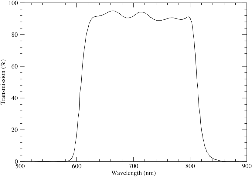
Figure 1: The transmission curve for the filter used on the BNPC.

The detector is a 4096 x 4096 front-illuminated, KAF-16801E chip with transparent gate (and thus a relatively high sensitivity for such a chip) and pixel dimensions of 9 $\times$ 9 $\mu$m, in an FLI camera. The image scale is 3.89$\arcsec$/pixel for a field of view of 19.6 square-degrees. The camera is equipped with a single filter, with peak transmission $\sim 705$ nm and HPFW $\sim 205$ nm, properties similar to those of the Johnson $R$ passband [700 and 200 nm, respectively; Drilling & Landolt (2000)]. See Figure 1 for a plot of the filter transmission, measured and replotted from a manufacturer supplied tracing.

2 The Variable Star Search Program

Previous survey work has involved searches for transient objects, and some have specifically targeted gravitational lensing events such as OGLE [FOR Optical Gravitational Lens Experiment; Udalski et al., (1993, 2002)]; and MACHO [for Massive Cold Halo Objects; Alcock et al. (1995)]. Others have targeted extrasolar planet transits, such as HATNet [for Hungary Automatic Telescope Network; Bakos et al. (2002, 2004a)] and TrES [for Transatlantic Extrasolar Planet Survey; Alfonso (2004)], as well as variable stars. One of the more comparable variable star surveys is the MOTESS-GNAT [for Moving Object and Transient Event Search System and Global Network of Astronomical Telescopes] survey (Kraus et al. 2007), although it currently involves three telescopes of 35-cm aperture, instead of one 50-cm telescope, as for the BNPC. Most such surveys make use of either small resolution, large field cameras with relatively bright faintness limits, as HATNet, or larger telescopes with smaller–field image cameras, as MACHO.

The BNPC has the great advantage of enabling a search field of more than 19 square degrees of sky per exposure, and yet of reaching relatively faint limits, so that it provides excellent opportunities to sample the variable star populations across large swaths of the sky.

As Kraus et al. (2007) note, programs such as this fill “… a unique niche in parameter space, observing with intermediate depth, …” as well as large area and flexible repetition strategy.

The initial field selected for the program contains two open clusters but its selection had more to do with its serendipitous placement in the sky when the BNPC had been sufficiently well adjusted to permit commencement of observations. This field is well off the galactic plane and more or less devoid of very bright stars, although not devoid of objects of interest. It contains, for example, the planetary transiting system HD 209458, regrettably overexposed in the images images reported on here, as are most of the known variable stars in this field.

Other fields we are observing include the extensive Hyades and Coma star cluster regions and selected regions at various galactic latitudes. The regions away from the plane can be expected to produce an increased relative number of population II variables, and, because of the inclusion of external galaxies, supernovae. The frames are being archived for future investigations.

Our main goal in this program, however, is to improve the database of fundamental parameters of stars through investigation of eclipsing and regularly pulsating variable stars. Table 1 summarizes the data obtained to date which are in various stages of image reduction and data analysis.

Limitations on variable star detections are discussed below, with emphasis on those found in the analysis of the first set of data of what we call RAO Field 1. These and subseqent data sets will be made available on–line.

3 Observations and Observational Constraints

The observations reported here were obtained over the JDN interval 2453271.5 to 2453305.5. The summary of these data is presented in Table 2. The differences in numbers of frames in Tables 1 and 2 are due to relatively poor focus for some of the frames counted in Table 1 which were omitted from the analysis discussed here.

By trial and error we find that in order to detect variations of a few percent or less, the effective faint raw magnitude limit is $R_{J}\approx{17}$, determined by the sky background and concomitant noise. The bright end of the range, $\sim{11.3}$, is established by saturation limits. The highest precision is to be expected for the brighter side of this range, and it is there where an extrasolar planetary transit may be detected, although this still relatively rare type of detection event is not the primary focus of our program.

The skies over the RAO, located in the foothills of the Canadian Rockies at an elevation of 1300 m, are frequently non-photometric in the classical photoelectric photometry sense. The observatory is located within 50 km of the outskirts of a major metropolitan city with large if increasingly ameliorated light pollution (the introduction of lower wattage, downward-projecting street lamps being the ameliorating factor). For this reason, the Rapid Alternate Detection System (RADS) for gated, pulse-counting differential photoelectric photometry of individual variable stars, was developed here (Milone & Robb 1983) because it eliminates first order extinction variation as well as sky brightness and its variation, except that occurring at the chopping frequency of the secondary mirror. One might expect that CCD photometry would allow one to correct for some of these effects, and, for this reason, comparison stars were taken as close to each variable candidate as was practical, as we describe below. However, the large field of view and small image scale have so far conspired to produce uneven results. Consequently, the nights we can actually use tend to be photometric in the classical sense of the word. Sky conditions, compounded by scheduling gaps, therefore, limit the precision of the data we have been able to acquire.

When the sky quality is high enough to justify observing, the large area detector CCD provides data on a large number of stars. The downside of the large sky field and consequent low spatial resolution is that even relatively sparse fields have to be treated as crowded ones. Thus, instead of the much-preferred multi-aperture photometry that involves what Stetson (1987) has called a “curve-of-growth” procedure, we have been able to apply only single aperture photometry. PSF fitting is now seen to be needed in order to reduce the effects of neighboring stars. However, PSF variations across the field produce additional complications, as we discuss below.

4 Image Analysis and Data Reduction

4.1 Image and Data Processing

The DAOPHOT package (Stetson 1987, 1990) within the IRAF data reduction package was used for the image processing. MDW wrote scripts to facilitate image processing and reduction calculations and to organize the results. The magnitudes were determined with a single 9-pixel aperture.

The raw magnitude of each star was converted into a differential magnitude with respect to a mean of $\sim{10}$ candidate comparison stars in the vicinity of each star image. The comparison star selection was automated and each of the ten had to meet the a number of criteria designed to assure constancy within precisional limits. Each candidate star needed to:

• have a signal-to-noise ratio better than the average;

• display differential light curves (with respect to the other stars) that deviate insignificantly from constant light;

• lay within 500 pixels of the program star; and

• produce differential light curves with the lowest standard deviation.

The last criterion, especially, has limited the number of comparison stars.

The differential magnitude was calculated from Equation 1.

$$DM_{i}=\frac{\sum_{j=0}^{j<n}{(M_{i}-k^{\prime}X)-(M_{i,j}^{c}-k^{\prime}_{i,j}X_{i,j}^{c})}}{n}$$ (1)

where $i$ indexes the candidate variable star, $j$ indexes comparison star, $n$ is the number of comparison stars (10, if possible, to beat down the effects of low amplitude stellar variation and such observational effects as residual psf variations across the field), $X$ is airmass, $k^{\prime}$ is linear extinction coefficient, and $M$, and $DM$ are the magnitude and the differential magnitude, respectively; the superscript $c$ refers to comparison stars.

4.2 Data Reduction

Our data have been corrected for extinction and have been approximately transformed to Johnson $R$ magnitudes.

For each night we calculated the Bouguer extinction coefficient (Bouguer 1729), $k\arcmin$, for each comparison star with a linear least squares fit and then performed a sigma clipped average of all the individual star $k\arcmin$ values to find the nightly $k\arcmin$ mean.

The zero point of the magnitude scale was determined by comparing our systemic magnitudes and the $R$ magnitudes tabulated in the USNO 2.0A catalog. There seemed to be no sensitivity to color in this zero point correction, as, for example, the color index term expressions given by Hardie (1962).

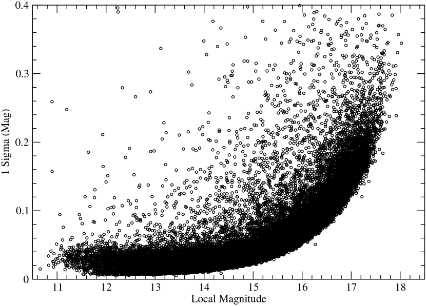
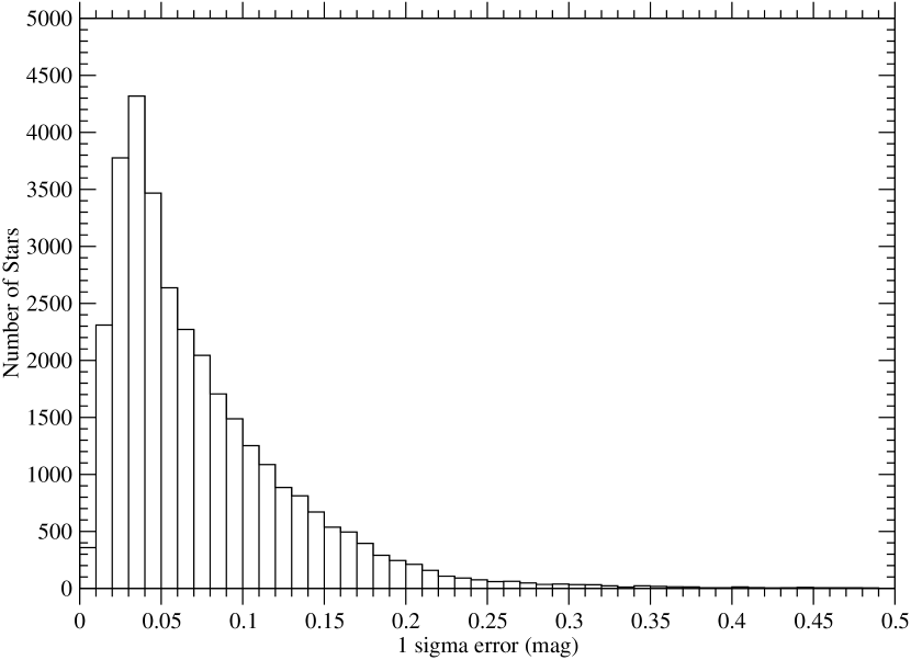
Figure 2: The precision as a function of magnitudes for the measured light curves (left) and the histogram of achieved 1 $\sigma$ levels in the light curves (right)

Figure 2 is a histogram of the 1$\sigma$ levels in the light curves as determined thus far.

5 Variability Detection and Analysis

The differential light curves were searched for periodic variations using the analysis of variations (ANOVA) technique outlined in Davies (1990, 1991) . This technique searches for periods with which a significant variation in mean values between different phase bins is produced.

Before each light curve was searched, it was clipped of points that exceeded 5$\sigma$ from the mean. If more than four points exceeded this limit, no points were clipped, limiting the clipping to solely erratic points.

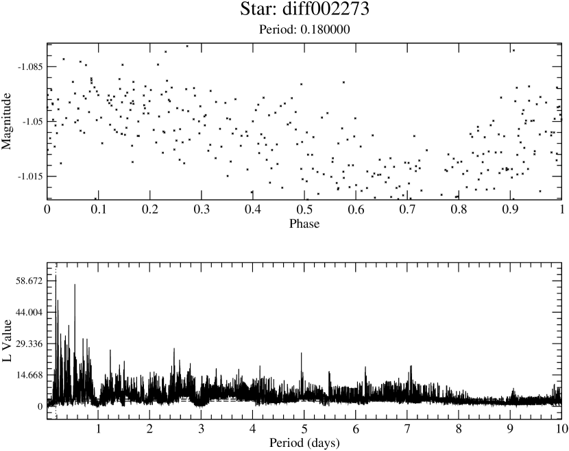
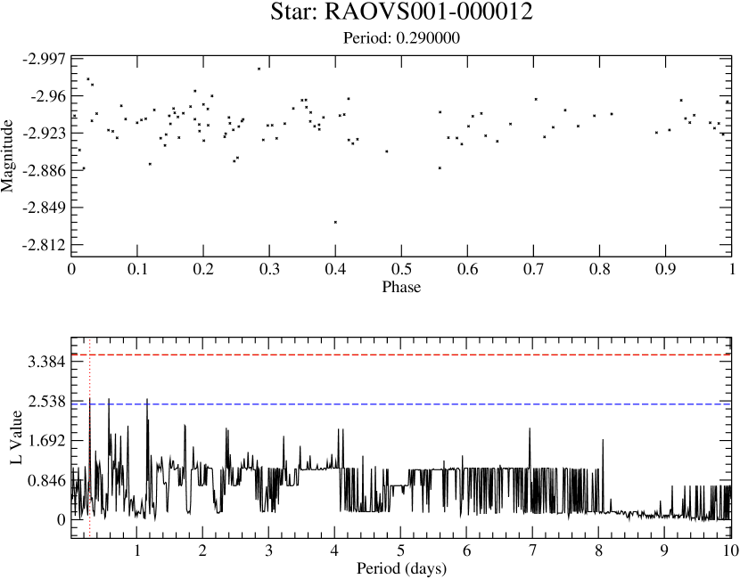
Figure 3: Two light curves and their L statistic plots that illustrate cases where variability is detected (left) and where no variability is detected (right). The phased light curves are plotted in the top graph. The horizontal dashed lines in the L statistic plots represent the 99% and 95% confidence levels for the lower (blue) and upper (red) lines, respectively (colors visible in the on-line version of this paper).

The search produces an L statistic value (Davies 1990) for each period searched (for examples see Figure 3); the larger the L statistic the greater the variability between phase bins. The test statistic follows an F distribution, which is used to determine if the L statistic value is indeed statistically significant. If the maximum test statistic for a certain light curve is significant then the detection routine marks that star as variable and records the period associated with the maximum as the period of variation.

The light curves were searched for a range of periods between 0.01 days and 10 days, in increments of 0.001 day. The phased light curves were divided into 5 bins and we looked for variations in the means among the bins to a significance level of 99%. For RAO Field 1, we initially detected apparent variability in 10,406 of the 26,271 stars searched. Such a high fraction of apparent variability was unexpected and disappointing. Thus the stars that were detected as variable had to be sifted further, individually. Most of this variability was found to be due to systematic noise sources. In many cases the systematic noise was due to light contamination from nearby stars and this can vary from frame to frame, primarily due to seeing variations.

The FWHM of a stellar profile can vary by as much as a factor 2 during a night. As the stellar FWHM increases, the level of contamination seen in the fixed aperture also increases: apparent variability in the light curves of stars that have bright near neighbors is induced by variability in their stellar profiles.

Typical FWHMs are 2.34 pixels, equivalent to 9.10$\arcsec$, at the center of the frame, and 3.77 pixels, or 14.67$\arcsec$, at the corners, but they do not vary smoothly across the image, and, in fact, the spatial variation differs during a night’s observing. Seeing (typically 3–4$\arcsec$ but variable) contributes to the large star images, but there appears to be an important instrumental contribution also.

To date, PSF fitting has proven both difficult and time consuming to apply reliably, due to the PSF variability. Nevertheless, the large number of stars that display systematic noise in light curves requires continued use of this method to reduce the effects of neighboring stars.

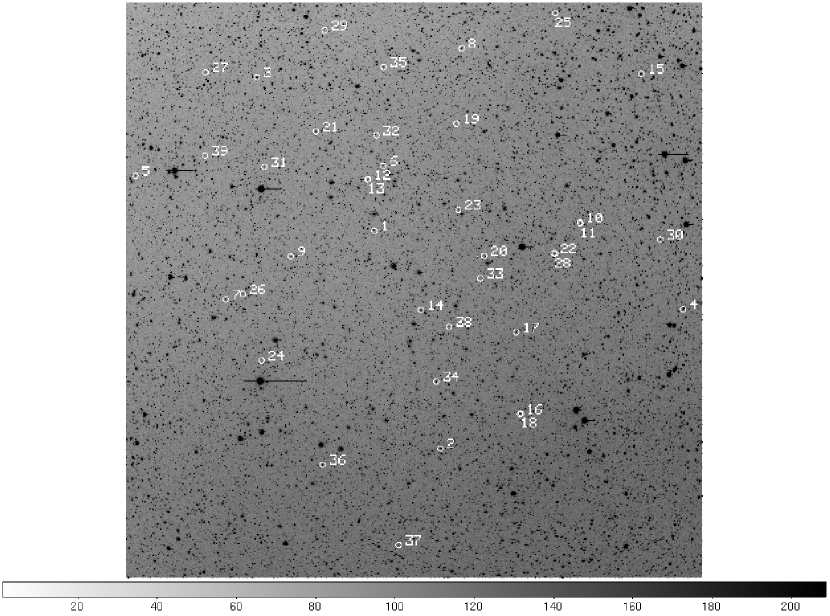
Figure 4: RAO Field 1 showing the detected variable stars

The detected variables and their determined properties are listed in Table 3. They are marked and labeled in Figure 4. The “Auto Period” is the period detected by the automatic search routine. The uncertainty (mse) is given in parentheses in units of the last decimal place.

The light curves of the detected variables were subsequently searched again, with more phase bins (40) and a finer period step (0.00001 day). The peaks in the array of test statistics were fit with Gaussian curves to estimate periods; in each case the uncertainty was found from the HWHM of the peak. The period column in Table 3 records this refined period. We obtained the epoch by fitting the deepest minimum (for binary stars) or the maximum (for pulsating variables) with a Gaussian function. The uncertainty in the epoch was the formal error in this fitting.

However, the small image scale requires that we place caveats on the discoveries of several pairs of close–neighbor stars in the variable star list. These include pairs RAO1-10 & -11, -12 & -13, -16 & -18, and -22 & -28. With the exception of pair RAO1-16 & -18, the stars making up these pairs had the same detection period, within the uncertainties. It is thus likely that only one star in each such pair is the true variable. The light from the variable star may contaminate the aperture of its non-variable neighbor of the pair, imparting its variation to an otherwise non-variable light curve; and the variable, in turn, may be contaminated with light of the non–variable. Both light curves will appear shallower then the undiluted light curve because of the added light, in a flux-weighted sort of way. Assuming that each of the pairs of objects we identify as producing a common light curve does represent only one intrinsically variable star, we are left with 35 apparently bonafide variable star detections.

6 Results: The Variables in RAO Field 1

6.1 Periodic Variables Found and Not Found

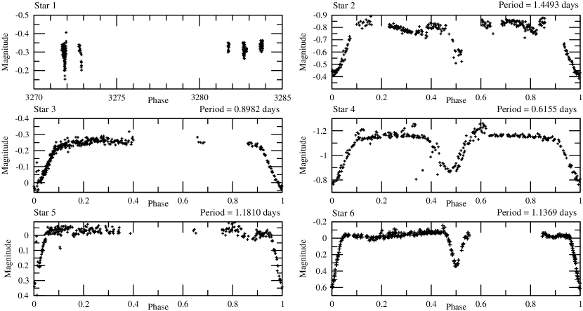
Figure 5: Detected variable stars with Algol (EA)–like light curves.

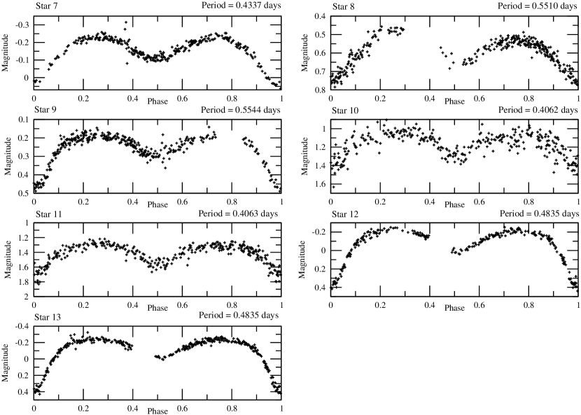
Figure 6: Detected variables with $\beta$ Lyrae (EB) light curves.

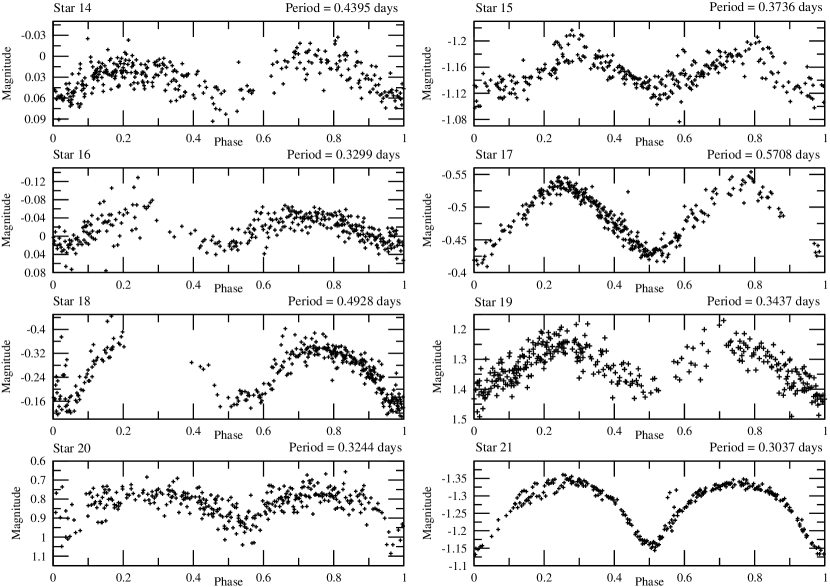
Figure 7: Detected variable stars with W UMa (EW)–like light curves.

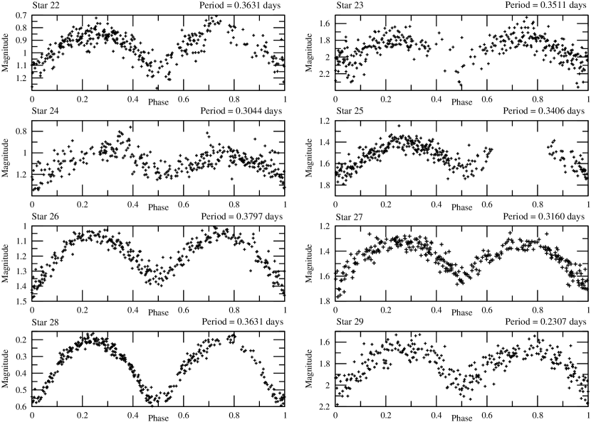
Figure 8: Detected variable stars with W UMa (EW)–like light curves.

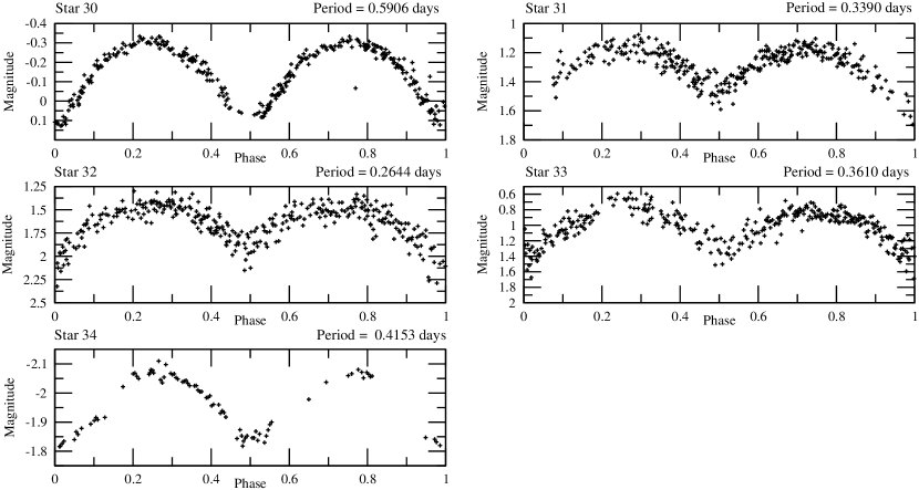
Figure 9: Detected variable stars with W UMa (EW)–like light curves.

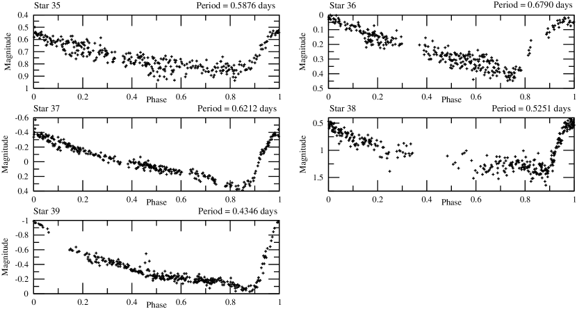
Figure 10: Detected variable stars with RR Lyr light curves.

Figures 5, 6, 7, 8, 9, and 10 are plots of the light curves for the stars in which we have detected variability, collected into light curve types. It will be noted that the variability of star RAO1-01 has not been phased, and its identification as an Algol light curve is tentative. The light curves of stars RAO1 -03 and -05 lack secondary minima, and, although smaller scatter favors the periods cited, these systems could have half the periods listed.

Table First Results from the RAO Variable Star Search Program. I. Background, Procedure, and Results from RAO Field 1 contains a list of the known variable stars in the search area, detected as periodic variables with the aid of the SIMBAD and AAVSO databases. The last column gives the RAO star number with which we can associate eleven of our detected periodic variables stars: RAO1-06, -07, -12, -15, -18, -21, -30, -34, -37, 38, and -39. In addition, two other variables we detected (-02 and -04) are in the vicinities of two known variables. This may account for some if not all the variation apparently superimposed on the eclipsing light curves of these two objects. Table First Results from the RAO Variable Star Search Program. I. Background, Procedure, and Results from RAO Field 1 does not contain stars that were over-exposed in our images except for two that lay close by the variables that we detected. Of the 23 variables stars in the list that were not over-exposed, we detected 20 of them, and resolved the variation in 16 of these. The variability in the remainder was masked by the noise sources discussed above.

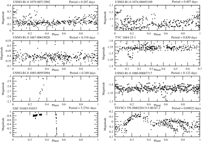
Figure 11: Light curves for the previously known variable stars that were not detected as periodic variables in our search. The light curves are phased with the literature period.

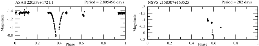
Figure 12: Light curves for the previously known variable stars that were not detected as periodic variables in our search.

Figures 11 and 12 show the light curves from our data (phased to the period given in the literature) for the ten previously known variable stars that we failed to detect as having periodic variability. In fact, all but three of these systems we classify as possible variables (marked “DP” in Table First Results from the RAO Variable Star Search Program. I. Background, Procedure, and Results from RAO Field 1) but the systematic noise in the light curves precluded reliable detection of any significant degree of periodicity. For example, stars TYC 1684-23-1 and GSC 01683-01853 exhibit significant variation, but not complete cycles in the present dataset. Many known variable stars are within the RAO1 field but nearly all are undetected because the images are saturated; in some cases the star may appear too bright due to the blends with bright objects in close proximity. For instance, for the “DN” case USNO-B1.0 1085-00593094, there are insufficient data obtained under good seeing conditions with which to do a period search because of the star’s proximity to an over–exposed star. NSVS 11679488 (2158307+163525) is classified as “M”, and is a long–period variable; this object was detected and Figure 11 shows some evidence of variation over the interval of our observations ($\sim{0.1}^{P}$), but hardly sufficient to see periodicity. USNO-B1.0 1080-00687717 (12.4 DSCT, “DN” in our table) does not show any coherent variation at the published period and should be reobserved carefully.

TSVSC1 TN002201313-80-67-2 has a clearly visible phase variation for part of a cycle, but is swamped by noise in the rest. Tycho 1683-00877-1 (11.40 EW, marked “N”) we have not detected, although its position places it near RAO1-04; it is at the bright limit, so is likely saturated in our image frames. ASAS 220539+1721.1 (12.40 ED, marked “DP”) was not detected to be variable, although we expected it to be. In these cases the threshold for variation was set too high to avoid false detections dur to variability in the stellar profiles.

One of the known systems which is overexposed is the extrasolar planet transiting system HD 209458, a system coincidentally studied by one of us for an MSc degree (Williams 2001).

Although the statistics of small numbers must be borne in mind, it is of interest to compare the relative frequencies of the types of variable stars we detected with those known from past compilations. For this purpose, we use primarily the nomenclature of the General Catalog of Variable Stars, and augmented by that in use at the SVX archive of the AAVSO website. From this source, the relative frequencies of short–period pulsating variables, and the EA/ED, EB, and EW/EC types of eclipsing variables should be: 69.5, 13.7, 8.1, and 8.6% of the total number of variables in these categories, so in this source we find the ratio of eclipsing to pulsating systems to be 0.44. However, we found also from the SVX site, the ratio of numbers of eclipsing systems (EA, EB, EW, EC, ED, and more general E categories) to short–period pulsating stars (DCEP, RR, RRA, RRAB, RRC, RRD, DSCT, and more general categories), to be 1.13. The ratio of numbers of the eclipsing binaries in the EA, EB, EC, ED, and EW subcategories alone) to only those in the RR Lyrae subtypes is 0.74. Yet we have classified 30 of the 35 detected variables to be eclipsing, so the ratio is 6:1. These comparisons suggest that in our preliminary survey results we are undersampling the number of pulsating stars.

RR Lyrae variables are more widely distributed in the galaxy, but, as giants, are more luminous, and so visible over a greater volume, than are the pairs of dwarfs making up overcontact systems, especially the most numerous of these systems, those with cool components. Typically, RR Lyraes have periods between 0.4 and 0.6 day but some subtypes peak at shorter periods; delta Scuti stars may have much shorter periods, whereas W UMa systems typically have periods between 0.2 and 0.4 day; systems with $\beta$ Lyrae light curves have a greater range of periods, and Algol-like light curve systems, an even greater range.

We now consider it unlikely that we have misidentified many pulsating light curves, especially those of the DSCT (delta Scuti) stars, as W UMa light curves, but some misidentifications are certainly possible, as is multiple variability. In the case of misidentification, the pulsating star’s period would be half that given in Table First Results from the RAO Variable Star Search Program. I. Background, Procedure, and Results from RAO Field 1. We note that several systems identified here as of EW type have nearly sinusoidal light curves and a number of these have shallow light curves. In an EW system, a low amplitude light curve implies low inclination, whereas in delta Scuti systems, low amplitudes are common. However, DSCT stars constitute 4.5% of all pulsating stars in the SVX survey and only 2.1% of the combination of short-period variables in the the pulsating and eclipsing variable star groups. In principle, other of our EW systems could be members of the subclass (RRC) of RR Lyrae stars; RRC stars have sinusoidal light curves with lower amplitudes (typically 0.5 magn) and constitute 10.2% of RR Lyrae type variables. Color information as well as spectroscopy can be used to discriminate between EW and RRC types, as pointed out some time ago by Wesselink et al. (1976).

The ellipsoidals are yet another class of variable with low-amplitude sinusoidal light curves. These are even rarer objects, however, making up less than 0.3% of short–period variables. Finally, some low-amplitude objects may be spotted, and relatively fast rotators. Where this is the case, the amplitudes and shapes should vary over cycles; low–amplitude candidates in our sample include stars RAO1-14, -16, and -20 (three of the 19 we intially classified as EWs) — all potential members of this group.

Three possiblities for the paucity of RR Lyrae stars in our data set are that:

1. There is a bias due to differences in spatial distribution. Objects of the old disk population, to which most of the dwarf binary systems likely belong, are more concentrated near the galactic equator than are population II RR Lyraes, which are more spherically distributed;

2. There is a luminosity bias in the survey because of our effective magnitude range. The more luminous RR Lyrae stars that are close to us are overexposed, whereas the more distant ones are preferentially dimmed and reddened as a consequence of being more distant and thus of having greater interstellar extinction than do the nearby overcontact binary star components;

3. There is a bias toward shorter period systems in our survey, favoring W UMa systems, for example, over the statistically slightly longer period RR Lyr systems.

The mean brightness of an RR Lyr star is $M_{V}\approx{0.7}$. The distant modulus range that we sample within the bright and faint magnitude limits of our survey is $10.6\leq(V-M_{V})\leq 16.3$ for the RR stars, and $7.2\leq(V-M_{V})\leq 12.9$ for a pair of solar–type stars, and for a mixed population of binaries over a range of 5 magnitudes of $M_{V}$, centered on $M_{V}$ = 6, $\sim{3}\leq(V-M_{V}\leq\sim{14}$. Interstellar extinction makes objects appear fainter and thus more distant, but the true volume is not plumbed more deeply, so that the number of stars is not thereby increased.

Regarding hypothesis 1, the galactic coordinates of RAO field 1 ($l_{II}$ = 76.8$\arcdeg$, $b_{II}$ = 28.5$\arcdeg$) place it $\sim{30}\arcdeg$ off the galactic plane, so that the frequency of old disk and younger objects relative to that of the RR Lyrae types should be decreased compared to the ratio in the galactic plane; howeve it will be large. The mainly dwarf type stars that constitute most of the binaries we detect can not be seen at distances as great as the RR stars. The slant direction thickness through the galaxy’s thick disk is double the path length through the normal to the galactic plane, and this certainly increases the numbers of detected dwarfs relative to RR stars. Therefore the hypothesis must be correct at some level, but it is hardly clear that it is quantitatively sufficient.

Hypothesis 2 also has merit because even with minimal extinction, the brightest RR Lyrae star that we can detect must be more than a kiloparsec away, if interstellar extinction is less than 0.5 magn, although there is a dependence on metallicity (Hall 2000, p.400). If we take into account that the RR Lyrae stars are themselves not uniform in spatial, metallicity, or period distributions, the argument become stronger. Classically there is a dichotomy in the RR Lyrae group (Gilmore & Zeilik 2000, p. 479) between RR stars with periods greater than $0.4^{d}$ for which the galactic scale height, $h$, is 2kpc, and those those with periods less than $0.4^{d}$, for which $h=300$ pc. These numbers can be compared with the scale height for old population I stars, 100 pc. The shorter period RR stars are said to be more numerous in the solar neighborhood, and these would be brighter as a consequence, so bright that they will exceed our bright limit. Because these stars are saturated on images, so they will not be measured and will not get into the database. The dust is confined primarily to the galactic plane, and the extinction in the plane is typically $\sim{1}~{}magn/Kpc$. Much of the extinction must be local, but the net result will be to decrease the numbers of the more distant stars; indeed, because the sample of stars is actually drawn from a segment of the celestial sphere with a smaller distance, the volume sampled will be smaller. Therefore this hypothesis, too, appears necessary but may not be sufficient to explain the full disparity.

Hypothesis 3 certainly applies, because the shorter-period RR’s are distributed closer to the plane, and these are too bright to be seen. All five of our detected RR stars have periods longer than $0.4^{d}$ (see Fig. 10). Thus it appears that all the hypotheses have merit because they involve closely correlated properties of the RR Lyrae stars. Again, the last hypothsis is necessary if not sufficient to explain the relative paucity of RR stars in our discovery list. The qualitative explanation may be correct, but a larger body of data will permit tests of the hypotheses. To that end, we are acquiring images with a range of exposure times, thus expanding the dynamic range of the brightness, and distance, of detected variables.

Looking now at the major subgroups in more detail, we see that among the EA, EB, and EW/EC cases in the SVX database, the percentages of these types are 33.4, 5.6, and 60.9%, respectively. This can be compared with 20, 17, and 63%, respectively, of our sample of the 30 independent variables detected according to our criteria. Therefore the number of over–contact systems we detect is as expected, whereas the Algols appear under-represented, and the $\beta$ Lyraes, overabundant, notwithstanding the statistical uncertainty in these small numbers. A relative paucity of Algol (EA) systems relative to W UMa (EW) systems, though, is not difficult to explain. The relatively short interval of observations and short durations of minima of the EA systems combine to limit the number of such systems that can be detected in our data. The distribution of periods is far greater for the Algols than for the W UMa types, so over short intervals the long–period Algols will be missed. Thus the discrepancy between EAs and EWs is readily explained, at least qualitatively.

Finally, this discussion has been about light curve as opposed to binary morphology. It is another matter entirely to identify systems not according to the shape of their light curves, but according to their state of binary evolution. The characteristic rounded maxima that signals a star’s departure from spherical shape is usually absent from the visual light curves of systems with Algol–like light curves: the hotter component is more luminous than its low–surface brightness companion, and dominates optical light curves. In infrared light curves, where a larger contribution comes from the larger, cooler component, the curvature is observed; in the IR, Algol itself is seen to have rounded maxima.

To identify the morphological types, and to aid in any further light curve studies, we have performed preliminary analyses of the detected eclipsing systems for which both minima are observed. The converged solutions may be useful as starting values for analyses of larger and more precise data sets, and to identify particularly interesting targets.

6.2 Preliminary Light Curve Analyses

Analyses were attempted on all the eclipsing binaries in Table 3 by EFM with the WD package described initially by Kallrath et al. (1998), and updated to include improvements up to 2007 (see Milone & Kallrath 2008). The package contains a simplex program, a Wilson–Devinney program (version $\sim{1998}$), a damped least–squares (DLS) version of the latter program, and a simulated annealing (SA) program, which, however, was used only sparingly in the present analyses. The SA program, described and illustrated in Milone & Kallrath (2008), is as robust a light curve solver as one may find, but it is not as efficient as the Simplex program at finding global solutions, and in the present application where a large number of light curves had to be analyzed, a starting run with the simplex routine usually sufficed.

In the present study, the simplex algorithm was run, preceding a self–iterating version of the Wilson–Devinney program; on completion, a final DC and LC run then gave the least-squares parameter values and their mean standard errors (mses). Either the simplex or the DLS iterations ended when either full convergence was obtained, i.e., when the correction for each parameter became less that its mse, or when one of the stopping criteria was reached. Stopping criteria include preset values of the number of iterations, the number of changes of the Marquardt damping factor, or an error limit, typically selected as the uncertainty in a single observational datum. The latter is compared to the mse of the fitting. The stopping criteria are stipulated in an information file, along with the programs to be used in sequence, the beginning CGS log g values for each component (automatically updated as the model changes during the calculation), the name of the flux file that contains the ratio of the atmospheric flux (from the models of Kurucz (1993) to that of a blackbody (in the present case, only that for the $R_{J}$ passband), and a number of other control parameters. The Differential Corrections (DC) input file and a constraints file which lists the ranges over which parameters may be varied to keep the exploration within realistic physical limits, are also required to run the package.

We typically started each system’s run in mode 2, in the parlance of the Wilson–Devinney program, which is appropriate for fully detached systems. These modes (and the models for which they are appropriate) are: 2 (detached system), 3 (overcontact), 4,5 (semi-detached with primary, secondary filling its Roche Lobe, respectively), and 6, for contact systems, where both stars fill their inner lobes and are thus in marginal contact. It is standard among light curve modelers to determine the proximity of the computed stellar radius to its inner Lagrangian surface, or Roche lobe, with the fill-out parameter, defined by

$$f=\frac{\Omega^{I}-\Omega}{\Omega^{I}-\Omega^{O}},$$ (2)

where $\Omega$ is the modified Kopal potential and $\Omega^{I}$ and $\Omega^{O}$ are the inner and outer Lagrangian surface potentials, respectively. Where f $\approx{0}$, the component is near its inner Lagrangian surface, and where f $>$ 0, it exceeds this limit. This quantity is computed in the simplex program output within the WD package.

If convergence was not achieved in mode 2 initially, we made further runs with the best values of the preceding run as starting parameters, with a recomputed semi–major axis from the new period value. At this point, the data set was reexamined and residuals that exceeded the Chauvenet criterion were given zero weight (although they still appear in the final fitting plots). If, after several such attempts, convergence was not achieved in mode 2, or if the fill–out parameter indicated that the components were close to or exceeded their Roche lobes, a run was made in the over–contact mode. Finally, when no convergence was found after several such attempts, or the fill–out parameters suggested them to be viable models, a run was made in modes 4, 5, or 6, as appeared appropriate.

In all the cases of the light curves identified as “WUMa” (“EW”) type, we have explored fittings with both detached (mode 2) as well as over-contact models (mode 3), and where f $\approx{0}$, for either or both components, we modeled the systems also in modes 4, 5, or 6.

In light curves where the maxima are curved, we attempted to model the photometric mass ratio among the full suite of parameters. In other cases, we modeled only the inclination, $i$, the temperature of the secondary component, $T_{2}$, the modified Kopal potential $\Omega_{1}$, the period, $P$, the epoch, $t_{0}$, and the passband luminosity, $L_{1}$. For detached systems, we adjusted also the potential of the secondary component, $\Omega_{2}$. We employ here the photometric definition of “primary” and “secondary” stars as those at superior conjunction at the primary (deeper) and secondary eclipse, respectively.

Because we have no color or spectral information about the primary component, in almost all cases, we arbitrarily set $T_{1}$ = 6000 K. The lone exception was RAO1-29, a faint, very short–period system, for which we set $T_{1}$ = 5000 K.

In all cases, the starting period and epoch are those derived by MDW and which appear in Table 3, in the “Final Period” column.

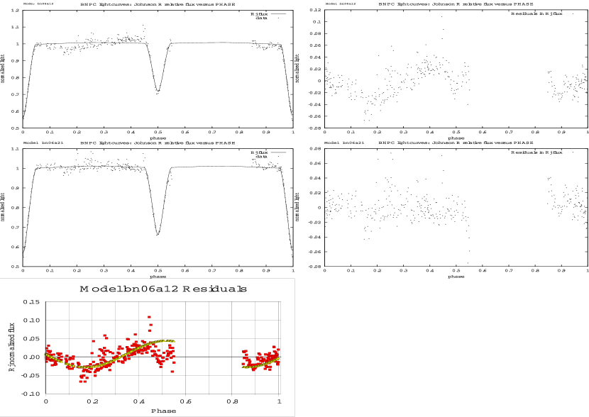
Figure 21: Light curve residuals for RAO1-06, model bn06a13 (with residuals included), top; for RAO1-06s, model bn06a21 (with a sinusoid fitting to the residuals removed), middle; and the empirical sinusoidal fitting of the residuals, bottom. See text for details.

The results of the analyses for 26 converged cases (iincluding two for RAO1-06, and one each for the duplicate pair RAO1-10 and RAO1-11) are listed in Table  5. The fittings and residuals of the fits are shown in Figures 13 – 21. The number of observations in the light curve appears in column 2 and the mode of the adopted model appears in column 3.

Although $T_{2}$ is listed as a parameter in the output lists of the DC program, in effect the program calculates only the difference in temperature between the two components, as determined primarily by the difference in depth of the two minima. Thus we list only the temperature difference, $\Delta$T = $T_{2}$ - $T_{1}$, and its uncertainty, in column 5.

The last column contains the standard deviation of a single observation of average weight. The other columns contain the parameters and their mse uncertainties. Where no uncertainty is given, the quantity was computed internally from other quantities or was assumed.

From the 25 converged solutions, we can categorize the systems: 10 detached, 3 semi–detached, 10 overcontact, and 2 contact systems. However, the detached systems RAO1-10 and -11 are very likely contain information about the same variable star, but contain the light of another object in either greater or less proportion, so that we actually have 24 independent systems (9 detached systems) for which solutions are found. Over–contact systems RAO1-22 and -28, for which the detection process found the same period, however, have produced different periods and other properties in the light curve analyses, and may well be independent variables, afterall. Next we will describe next some of the potentially most interesting systems to emerge from the analyses.

6.3 Solutions

The light curve of RAO1-04 is distorted with what appear to be variations in system light, so the data with the worst residuals were given zero weight. The slight curvature at maximum light makes the direct determination of mass ratio as one of the simultaneously adjusted parameters problematic. In such a case, however, a grid search, where only one parameter can be adjusted, can be performed over a range of values to find a minimum sum of squares of residuals (SSR). For RAO1-04, $q$ was adjusted in 20 trials across the range 0.75 $\leq$ q $\leq$ 1.30 to determine the mass ratio for RAO1-04. Optimization was achieved for q = 1.1 in this detached system, which shows only a slight curvature in the maxima. The fitting and residuals plots can be seen in Fig. 13.

One of the more interesting systems is RAO1-06, a detached system, which in the adopted model has residuals that appear to follow a sinusoid, indicating a possible low-amplitude variable in the system. The photometric mass ratio could not be determined in this system from the single $R_{J}$ passband and single epoch light curve alone, and so was assumed to be 1 and not adjusted. The earlier modeling trials for RAO1-06 assumed a more complicated reflection solution than is usually assumed in an attempt to reproduce the apparent positive slope in the light curve between phases 0 and 0.5. Usually a large “reflection effect” occurs in systems with a large difference in sizes and temperatures of the components. However, in this case, results of early trials indicated these differences to be relatively small, and enhanced reflection treatment did not, in fact, diminish the residuals. The parameters for the best–fitting model to this point, bn06a13, is listed in Table 5 on the RAO1-06 line. It was possible to reduce the effects of the residuals by subtracting the following function:

$$f(res)=-0.036\times{sin~{}(1.45\phi)}~{}+~{}0.008$$ (3)

where $\phi$ is the phase in radians. This quantity was subtracted from the light curve to create the results listed for the object RAO1-06s; the fitting and residuals as well as the sinusoid superimposed on the residuals of model bn06a13 are shown in Figure 21. The eclipsing light curve is incomplete, so not too much should be made of this sinusoid representation beyond that further observations of this system are warranted.

The systems RAO1-07 and -12 were modeled as semi–detached cases after detached and overcontact models failed to produce convergence. For RAO1-07, the fill–out parameters were $f_{1}$ = -0.18 and $f_{2}$ = +0.06; the former value indicates that the primary component is within its Roche lobe, and the latter value indicates that the secondary component just slightly exceeds its Roche lobe. Although no solution was obtained in mode 3, the model was not far, in fact, from convergence. In the case of RAO1-12, the light curve is missing part of the secondary maximum (the maximum following the secondary minimum), but the other parts of the light curve could be well–fitted with the semi–detached model bn12a11. A converged solution was found also in mode 2, but the fitting was not as good as that for mode 5. The fill–out parameters for the mode 5 model were $f_{1}$ = -1.34 and $f_{2}$ = +0.03. The fittings for the systems’ converged solution models, bn07a14 and bn12a11, can be seen in Figs. 13 for RAO1-07, and 14 for RAO1-12, respectively.

Analyses of RAO1-22 failed to yield a converged solution in any mode until the SA program was invoked. Although running time in the WD package usually required less than 10 minutes, this run required $2^{h}47^{m}$. It too did not achieve convergence before the stopping criteria kicked in, but the adjustments indicated an area of parameter space not hitherto pursued, which is, indeed, the great value of the simulated annealing algorithm. The $T_{2}$ result indicated a higher value than had been seen before and suggested a different course of action. The the next run, the initial epoch was decreased by $P/2$, so that the minima became reversed; after a number of simplex trials, a converged solution was found for RAO1-22 with the properties shown in Table 5. Although many of the parameters of this system and RAO-28 are significantly different, they both required that $T_{2}$ be greater than $T_{1}$ (at least initially for RAO1-22). RAO1-22 exhibits a shallower and noisier light curve than RAO1-28 but these properties are insufficient to decide the issue. Thus despite the diffeences in modeled parameters, the jury is still out on separate identity for these variable stars. The fittings for models bn22a20 and bn28a14 can be seen in Figs. 17 and 19, respectively.

RAO1-23 is the sole system which converged in (and thus far only in) mode 4. Its large $\Omega_{2}$, $T_{2}$, and $L_{1}$ parameters indicate a hot subdwarf secondary component; the more luminous primary component fills it Roche lobe. The fill–out parameters were $f_{1}$ = +0.08, and $f_{2}$ = -0.003, very close to a mode 6 condition. The mass ratio q = 0.92, indicates that the smaller component is slightly less massive. The sparse secondary minimum is modeled as flat and somewhat deeper than the primary minimum. Should more data support this model, the light curve could be rephased to zero at secondary minimum, and the epoch altered by P/2; these changes would turn the system into a mode 5 model. However the high scatter in the light curve and lack of much data in the secondary minima result in large uncertainties, especially in $\Omega_{2}$, and thus in the radius of the smaller component. If the model survives additional observational and analytical scrutiny, this system would be a candidate for a multi–wavelength campaign. The fitting for model bn23a17 can be seen in Fig. 17.

RAO1-25 was successfully modeled as an overcontact system even though much of maximum 2 is absent; the fitting can be seen in Fig. 18.

In two cases (RAO1-30, and -33), both components appeared to be close to their inner lobes, and after trials with modes 2, 3, and 4 or 5, runs with mode 6 were attempted. Convergence was obtained in this mode alone for both systems. The result is interesting because very few systems are thought to be in a marginal contact state, with essentially zero thickness of the neck between them. If this result withstands analyses with more observations, these systems may be at cusps in their binary evolution, and will be important to monitor in the future. The fittings for these systems can be seen in Figures 19 and 20, respectively.

6.4 Non–solutions

The systems for which solutions could not be obtained are: RAO1-01, -02, -03, -05, -08, -13, -15, -18, -34. The light curves of RAO1-01, -03, and -05 probably lack two minima, and that of -02 as well as -04 show significant extra–eclipse variability, perhaps due to the proximity of known nearby variables. RAO1-02 and -04 should be observed in future to disentangle the types and perhaps modes of variability. As noted above, the RAO1-04 light curve distortion was not so great that a converged solution could not be obtained.

In RAO1-08, a spot on the secondary star was used to model the observed difference between the maxima. However, the insertion of a spot did not result in a convergent solution in this case. Asymmetries in several other light curves (RAO1-07, -08, -10, -14, -16, -24, and -33), suggest the presence of starspots also, but in most of these cases the systematic difference between the maxima [long ago designated the “O’Connell effect” (Davidge & Milone 1984)] was small enough that specific spot modeling was not needed to achieve convergence. In some cases, as in RAO1-14, the asymmetry shows up mainly with a larger scatter in one maxima than in the other.

RAO1-13 appears to be a semi-detached system; the adjustment for the passband luminosity alone could not be brought lower than the mse in that parameter, and thus prevented convergence.

The peaked light curve of RAO1-15 could not be fitted in modes 2 or 3, and its relatively shallow light amplitude may be due to intrinsic variability, even though previously classified as EW and EC/?.

RAO1-18 seems to require an eccentric orbit to explain its displaced secondary minimum, but despite considerable effort to solve it, convergence could not be obtained for this system. In any event, the light curve is incomplete and analysis requires more data.

The data available for RAO1-34 is rather sparse, so it is probably not surprising that convergence was not achieved for this system.

7 Conclusion

To carry forward our discussion of morphological types of binaries in Section 6.1, we note that the proportions of converged systems in the modes 2: 4+5: 3+6 is 10:3:11 or roughly 42:13:46%, based not on light curve shape, but on physical morphology. These can be compared to the ratio of these systems from the Koch et al. (1970) Catalogue of Graded Photometric Studies of Close Binary Systems: 30:23:47%, proportions investigated some time ago by Linnaluoto & Vilhu (1973) . By this measure, the detached systems appear slightly overabundant, and the semi-detached systems slightly underabundant in our sample. However, both samples are small ones: the movement of one star out of one category and into another in our sample produces a relative change of 6%. For our sample, therefore, it is clear that the apparent difference in frequency distribution among morphological eclipsing variable types is not significant.

In Section 5, we noted the detection of likely duplicate variability in several of the identified stars: RAO1-10 and -11; -12 and -13; -16 and -18, and -22 and -23. Converged solutions were found for only one of each pair except for RAO1-10 and -11, and -22 and 28; for the former pair, the parameters agree within $\sim{2\sigma}$ for the most part. For the latter pair, there appear to be significant differences, casting some doubt on the duplicate hypothesis for this pair. The light curve of RAO1-10 was also found to converge when run in mode 3, but with larger fitting error. We therefore report only the detached solution elements for this system in Table 5.

The low angular resolution of the BNPC frames compels us to treat the images as crowded fields with single-aperture image analysis. Therefore, the preferred treatment for precise image analysis, multi-aperture photometry, that involves a “curve-of-growth” procedure (Stetson 1987) that involves an extrapolation to include all of a star’s light, cannot be applied except for individual cases. A more generally applicable approach is point-spread-function (PSF) fitting photometry, a method that needs to be applied in order to remove the effect of neighboring stars. The clear need for this is illustrated by five of our discoveries. The difficulty in implementing application of this process generally is that the PSF is variable not only across the field but also from frame to frame, possibly as a result of instrumental flexure as the BNPC and the detector change hour angle. However, seeing variation contributes heavily to this large point spread function variation and this suggests that moving the instrument to a site with systematically better seeing could improve the central FWHM, and decrease some of its variation, by up to 50%.

In later image frames than we have discussed here, we have taken shorter exposures as well as longer exposures, to improve the dynamical range of detections. These later exposures will permit us to find longer-period variables. As with other searches, our period search method precludes eruptive or irregular variable stars. Many of these objects may show up, however, in a longer time base of observations. A larger database will also be able to test the hypothesis that our search methods appear to favor shorter–period systems.

Despite formidable difficulties, we have detected in our first run in this first field 35 variable stars, of which 25 appear to be new discoveries. In later reports, we will discuss other fields and results of analyses of data with longer time-bases.

Follow-up multi-color photometry is planned for all the variables with the newly refurbished 0.4-m and 1.8-m telescopes of the RAO, and radial velocity spectroscopy elsewhere. These will permit more complete light curve analysis to be carried out for all classes of variables found here in order to determine their fundamental properties, and to confirm the interesting discoveries about some of them.

To aid in those further studies, we have performed preliminary analyses of the eclipsing systems for which both minima are observed. These may be useful as starting values for more thorough analyses. Although the results must be regarded as preliminary, the analyses have identified a number of potentially interesting targets for further study. These include the apparent double–contact systems RAO1-30 and -33, the detached system RAO1-06 with sinusoidal light curve variation, and the apparent subdwarf semi–detached system RAO1-23.

For five variables that were previously reported, namely RAO-06, -07, -12, -21, and -30 (see Table First Results from the RAO Variable Star Search Program. I. Background, Procedure, and Results from RAO Field 1 for the literature names of these objects), we present the first light curve analyses. In each case, we confirm and refine the classification.

Finally, for those who desire to carry out their own analyses, the reduced data may be found at the website:

www.ucalgary.ca/~williamd/data/BNPC_paper1

Figure 13: Light curves and fittings (left) and residuals (right) for the eclipsing binaries for which we have obtained converged solutions: The fittings for RAO1-04, -07, and -09. The light curves are phased with the elements found in the light curve fittings.

Figure 14: Light curves and fittings (left) and residuals (right) for the eclipsing binaries for which we have obtained converged solutions: RAO1-10, -11, and 12. The light curves are phased with the elements found in the light curve fittings.

Figure 15: Light curves and fittings (left) and residuals (right) for the eclipsing binaries for which we have obtained converged solutions: RAO1-14, -16, and -17. The light curves are phased with the elements found in the light curve fittings.

Figure 16: Light curves and fittings (left) and residuals (right) for the eclipsing binaries for which we have obtained converged solutions: RAO1-19, -20, and -21. The light curves are phased with the elements found in the light curve fittings.

Figure 17: Light curves and fittings (left) and residuals (right) for the eclipsing binaries for which we have obtained converged solutions: RAO1-22, -23, and -24. The light curves are phased with the elements found in the light curve fittings.

Figure 18: Light curves and fittings (left) and residuals (right) for the eclipsing binaries for which we have obtained converged solutions: RAO1-25, -26, and -27. The light curves are phased with the elements found in the light curve fittings.

Figure 19: Light curves and fittings (left) and residuals (right) for the eclipsing binaries for which we have obtained converged solutions: RAO1-28, -29, and -30. The light curves are phased with the elements found in the light curve fittings.

Figure 20: Light curves and fittings (left) and residuals (right) for the eclipsing binaries for which we have obtained converged solutions: RAO1-31, -32, and -33. The light curves are phased with the elements found in the light curve fittings.

Table 1: Summary of RAO BNPC Data in all RAO fields

RAO Field	center $\alpha$ & $\delta$	JDN at 0h UT	Exposure (seconds)	Number of Frames
1	22:03:24 +18:54:32	2453256.5	60	7
1	22:03:24 +18:54:32	2453271.5	60	95
1	22:03:24 +18:54:32	2453272.5	60	70
1	22:03:24 +18:54:32	2453281.5	60	55
1	22:03:24 +18:54:32	2453282.5	60	75
1	22:03:24 +18:54:32	2453283.5	60	80
7	06:27:00 +52:30:00	2453305.5	60	30
8	06:27:00 +48:30:00	2453305.5	60	30
1	22:03:24 +18:54:32	2453305.5	60	36
2	22:03:24 +22:54:32	2453305.5	60	36
3	00:27:25 +25:36:44	2453310.5	60	45
4	00:27:25 +29:36:44	2453310.5	60	45
5	03:19:46 +36:53:48	2453313.5	60	52
6	03:19:46 +32:53:48	2453313.5	60	52
9	01:57:54 +37:39:28	2453965.5	60	42
10	18:01:09 +02:54:02	2453965.5	60	30
10	18:01:09 +02:54:02	2453966.5	60	42
9	01:57:54 +37:39:28	2453972.5	60	27
10	18:01:09 +02:54:02	2453972.5	60	18
10	18:01:09 +02:54:02	2453973.5	60	12
9	01:57:54 +37:39:28	2453974.5	60	6
10	18:01:09 +02:54:02	2453974.5	60	24
1	22:03:24 +18:54:32	2453981.5	60	40
2	22:03:24 +22:54:32	2453981.5	60	40
1	22:03:24 +18:54:32	2453982.5	60	53
2	22:03:24 +22:54:32	2453982.5	60	53
10	18:01:09 +02:54:02	2453981.5	60	36
12	12:22:39 +25:49:28	2454226.5	30	6
10	18:01:09 +02:54:02	2454270.5	10,60	4,21
10	18:01:09 +02:54:02	2454288.5	10,60	5,29
1	22:03:24 +18:54:32	2454307.5	60	9
2	22:03:24 +22:54:32	2454307.5	60	9
1	22:03:24 +18:54:32	2454308.5	60	28
2	22:03:24 +22:54324	2454308.5	60	28
10	18:01:09 +02:54:02	2454308.5	10,60	6,12
10	18:01:09 +02:54:02	2454309.5	10,60	9,17
1	22:03:24 +18:54:32	2454342.5	60	37
2	22:03:24 +22:54:32	2454342.5	60	37
1	22:03:24 +18:54:32	2454343.5	60	31
2	22:03:24 +22:54:32	2454343.5	60	31
1	22:03:24 +18:54:32	2454363.5	60	31
2	22:03:24 +22:54:32	2454363.5	60	31
11	04:25:02 +16:59:20	2454455.5	30,60,120	37,36,34
7	06:27:00 +52:30:00	2454456.5	60	86
8	06:27:00 +48:30:00	2454456.5	60	86
11	04:25:02 +16:59:20	2454463.5	30,60,120	18,18,18
11	04:25:02 +16:59:20	2454465.5	30,60,120	22,21,21
7	06:27:00 +52:30:00	2454466.5	60	28
8	06:27:00 +48:30:00	2454466.5	60	28
11	04:25:02 +16:59:20	2454467.5	30,60,120	47,47,47
12	12:22:39 +25:49:28	2454594.5	30,60,120	16,16,16
12	12:22:39 +25:49:28	2454607.5	30,60,120	6,6,6

Table 2: Summary of Exposures for RAO Field 1 Data Reported in this Work

JD at 0h UT	Length of Observing (hours)	Number of Observations
2453271.5	6.1	92
2453272.5	4.8	56
2453281.5	1.7	24
2453282.5	5.3	74
2453283.5	4.9	78
2453305.5	1.1	16

Table 3: Stars in RAO Field 1 in which we have detected variability.

Star	$\alpha$	$\delta$	Mag.	Auto Period	Final Period	Epoch	Depth(s)	rms	LC Type
RAO1-					(days)	(days)	(mag)	(mag)
01	22 03 47.7	19 09 14	12.27	0.3349	…	2453271.87$\pm$0.08	0.10$\pm$0.04, N/A	0.03	Algol
02	22 01 42.6	17 28 44	12.55	3.4306	1.4493$\pm$0.0029	2453283.74$\pm$0.05	0.26$\pm$0.03, N/A	0.02	Algol
03	22 07 36.2	20 20 09	12.33	0.4499	0.8982$\pm$0.0024	2453271.81$\pm$0.04	0.27$\pm$0.05, N/A	0.03	Algol
04	21 53 47.9	18 31 26	11.63	0.3179	0.6155$\pm$0.0029	2453272.79$\pm$0.03	0.36$\pm$0.02, 0.26$\pm$0.02	0.02	Algol
05	22 11 35.5	19 34 30	12.94	0.5899	1.181	2453271.81$\pm$0.03	0.36$\pm$0.03, N/A	0.02	Algol
06	22 03 30.2	19 39 11	12.97	0.3852	1.1368957	2453282.68$\pm$0.01	0.59$\pm$0.04, 0.39$\pm$0.03	0.03	Algol
07	22 08 03.8	18 37 42	12.56	0.4518	0.4337$\pm$0.0012	2453283.81$\pm$0.21	0.27$\pm$0.02, 0.12$\pm$0.02	0.01	$\beta$ Lyrae
08	22 00 54.6	20 33 08	13.00	0.2756	0.5510$\pm$0.0021	2453271.78$\pm$0.05	0.27$\pm$0.03, 0.17$\pm$0.02	0.02	$\beta$ Lyrae
09	22 06 30.9	18 57 31	13.11	0.5563	0.5544$\pm$0.0019	2453283.73$\pm$0.04	0.28$\pm$0.02, 0.10$\pm$0.04	0.02	$\beta$ Lyrae
10	21 57 06.9	19 12 16	14.37	0.1688	0.4062$\pm$0.0018	2453283.76$\pm$0.03	0.33$\pm$0.10, 0.24$\pm$0.07	0.07	$\beta$ Lyrae
11	21 57 05.5	19 11 48	14.02	0.2032	0.4063$\pm$0.0009	2453272.79$\pm$0.03	0.42$\pm$0.08, 0.27$\pm$0.06	0.05	$\beta$ Lyrae
12	22 04 00.8	19 32 51	13.05	0.3183	0.4835$\pm$0.07	2453271.75$\pm$0.02	0.60$\pm$0,04, 0.23$\pm$0.03	0.03	$\beta$ Lyrae
13	22 03 59.6	19 33 05	12.97	0.2468	0.4835$\pm$0.0007	2453271.75$\pm$0.01	0.61$\pm$0.03, 0.21$\pm$0.02	0.02	$\beta$ Lyrae
14	22 02 18.0	18 32 38	12.73	0.2199	0.4395$\pm$0.0015	2453271.78$\pm$0.25	0.04$\pm$0.02, 0.04$\pm$0.03	0.01	W UMa
15	21 55 01.6	20 20 22	11.44	0.1551	0.3736$\pm$0.0016	2454282.82$\pm$0.17	0.06$\pm$0.03, 0.06$\pm$0.02	0.02	W UMa
16	21 59 08.2	17 44 16	12.52	0.1674	0.3299$\pm$0.0013	2453283.76$\pm$0.12	0.06$\pm$0.04, 0.06$\pm$0.04	0.03	W UMa
17	21 59 13.3	18 22 01	12.20	0.8762	0.5708$\pm$0.0020	2453272.73$\pm$0.82	0.11$\pm$0.01, 0.10$\pm$0.01	0.008	W UMa
18	21 59 05.5	17 44 30	12.58	0.2463	0.4928$\pm$0.0021	2453283.75$\pm$0.05	0.15$\pm$0.06, 0.16$\pm$0.04	0.04	W UMa
19	22 01 06.2	19 58 21	14.00	0.1718	0.3437$\pm$0.0010	2453283.74$\pm$0.06	0.15$\pm$0.06, 0.12$\pm$0.04	0.04	W UMa
20	22 00 14.3	18 57 23	13.73	0.1395	0.3244$\pm$0.0009	2453271.88$\pm$0.03	0.16$\pm$0.11, 0.13$\pm$0.08	0.07	W UMa
21	22 05 41.9	19 55 08	11.41	0.1518	0.3037$\pm$0.0006	2453272.87$\pm$0.08	0.19$\pm$0.01, 0.17$\pm$0.01	0.009	W UMa
22	21 57 58.6	18 58 10	14.00	0.1816	0.3631$\pm$0.0010	2453283.69$\pm$0.09	0.24$\pm$0.09, 0.27$\pm$0.11	0.06	W UMa
23	22 01 04.0	19 18 40	14.92	0.1752	0.3511$\pm$0.0015	2453282.72$\pm$0.03	0.25$\pm$0.14, 0.28$\pm$0.19	0.10	W UMa
24	22 07 27.7	18 09 35	14.45	0.1305	0.3044$\pm$0.0011	2453271.89$\pm$0.05	0.27$\pm$0.11, 0.21$\pm$0.09	0.08	W UMa
25	21 57 49.0	20 48 59	14.22	0.1704	0.3406$\pm$0.0015	2453271.74$\pm$0.04	0.29$\pm$0.08, 0.23$\pm$0.09	0.06	W UMa
26	22 08 04.5	18 40 13	13.86	0.1898	0.3797$\pm$0.0009	2453271.88$\pm$0.03	0.31$\pm$0.06, 0.25$\pm$0.05	0.04	W UMa
27	22 09 19.1	20 22 27	14.06	0.1580	0.3160$\pm$0.0012	2453282.71$\pm$0.03	0.31$\pm$0.08, 0.23$\pm$0.07	0.05	W UMa
28	21 57 56.0	18 58 04	13.37	0.1816	0.3631$\pm$0.0005	2453272.79$\pm$0.03	0.35$\pm$0.03, 0.35$\pm$0.04	0.02	W UMa
29	22 05 24.3	20 41 47	14.72	0.1152	0.2307$\pm$0.0007	2455272.74$\pm$0.01	0.38$\pm$0.12, 0.30$\pm$0.10	0.08	W UMa
30	21 54 29.8	19 03 48	12.75	0.2955	0.5906$\pm$0.0013	2453283.77$\pm$0.04	0.39$\pm$0.04, 0.37$\pm$0.03	0.03	W UMa
31	22 07 22.6	19 38 47	14.31	0.1448	0.3390$\pm$0.0012	2453282.85$\pm$0.25	0.40$\pm$0.10, 0.26$\pm$0.09	0.06	W UMa
32	22 03 43.0	19 53 10	14.73	0.1322	0.2644$\pm$0.0007	2453271.73$\pm$0.01	0.59$\pm$0.19, 0.41$\pm$0.14	0.12	W UMa
33	22 00 22.2	18 47 00	14.75	0.1805	0.3610$\pm$0.0011	2453271.86$\pm$0.01	0.63$\pm$0.19, 0.50$\pm$0.19	0.13	W UMa
34	22 01 49.4	17 59 41	11.45	0.2619	0.3439$\pm$0.0018	2453271.71$\pm$0.18	0.24$\pm$0.03, 0.22$\pm$0.03	0.09	W UMa
35	22 03 28.2	20 24 44	13.70	1.2664	0.5876$\pm$0.0029	2453283.80$\pm$0.09	0.30$\pm$0.04	0.03	RR Lyrae
36	22 05 29.8	17 21 33	13.08	0.6799	0.6790$\pm$0.0028	2453272.78$\pm$0.19	0.37$\pm$0.03	0.02	RR Lyrae
37	22 03 04.0	16 44 18	13.32	0.6527	0.6212$\pm$0.0018	2453271.83$\pm$0.07	0.71$\pm$0.07	0.05	RR Lyrae
38	22 01 23.7	18 24 49	14.63	0.5243	0.5251$\pm$0.0015	2453271.76$\pm$0.03	0.83$\pm$0.13	0.09	RR Lyrae
39	22 09 19.0	19 43 56	13.49	0.4349	0.4346$\pm$0.0009	2453283.80$\pm$0.04	0.90$\pm$0.03	0.02	RR Lyrae

.

Table 4: Known variable stars in RAO Field 1.

Star	$\alpha$	$\delta$	Lit. type	$\lambda$ Mag.	Lit. Period	Ref	Status	RAO1-
GSC 01683-01853	21 53 23.67	+17 30 20.2	U	V 13.00-?	5.276	5	DP	…
= 1SWASP J21532.65+173020.3
TYC 1683-00877-1	21 53 45.20	+18 31 58.5	EW	w 11.40	0.587	2	N	…
USNO-B1.0 1080-00687717	21 53 58.91	+18 02 23.9	DSCT	w 12.39-?	0.122	2	DN	…
USNO-B1.0 1090-00579466	21 54 29.83	+19 03 52.0	EW?	w 12.88-?	0.566	2	DY	30
= ASAS 215430+1903.8?	21 54 30	+19 03 49	EC	V 12.76-13.26	0.591	6	(DY)	(30)
TYC 1687-1479-1	21 55 01.25	+20 20 25.7	EW	w 12.05-?	0.342	2	DY	15
= ASAS 215501+2020.5?	21 55 01.00	+20 20 30	EC/?	V 11.51-11.79	0.274	10	(DY)	(15)
USNO-B1.0 1067-00619020	21 58 16.32	+16 45 58.4	U	w 12.72-?	0.318	2	DP	…
NSVS 2158307+163525	21 58 30.14	+16 35 25.4	M	V 9.30-11.97	282.	7	DY?	…
USNO-B1.0 1067-0619189	21 58 54.40	+16 43 37.4	U	w 12.50-?	0.443	2	DY	…
USNO-B1.0 1077-00719427	21 59 05.41	+17 44 32.6	EW	w 12.91-?	0.407	2	DY	18
TSVSC1 N-N002201313-80-67-2	21 59 44.84	+19 30 25.5	U	V 14.88-?	0.698	8	DP	…
TSVSC1 N-N002201123-57-67-2	22 01 23.65	+18 24 57.8	U	V 14.44-?	0.525	8	DY	38
USNO-B1.0 1074-00692109	22 01 39.78	+17 28 33.7	U	w 12.54-?	0.407	2	DP	…
TYC 1684-522-1	22 01 49.27	+17 59 42.1	EW	w 12.12-?	0.415	2	DY	34
= GSC 01624-00522	22 01 49.25	+17 59 42.0	EW	V 11.77-12.08	0.415	11	(DY)	(34)
= ASAS 220149+1759.7
USNO-B1.0 1079-00712902	22 01 51.22	+17 58 53.7	U	w 12.56-?	0.207	2	DP	…
TYC 1684-23-1	22 01 54.39	+18 10 31.4	E	w 12.61-?	0.830	2	DP	…
ASAS 220304+1644.4	22 03 04.	+16 44 24	RRAB	V 13.07-14.11	0.621	6	DY	37
USNO-B1.0 1096-00579000	22 03 30.28	+19 39 12.8	EA	w 13.76-?	1.137	2	DY	6
= NSVS 11747875
NSVS 11748364	22 03 59.56	+19 33 07.2	EA/EB	w 13.46-?	0.484	7	DY	12
ASAS 220539+1721.1	22 05 39.	+17 21 06.	ED	V 12.40-12.94	2.805	6	DP	…
USNO-B1.0 1099-00576195	22 05 41.83	+19 55 10.9	EW	w 12.13-?	0.310	2	DY	21
= ASAS 220542+1955.2
USNO-B1.0 1085-00593094	22 08 25.85	+18 34 57.4	EW	w 11.46-?	0.349	2	DN	…
NSVS 11753088	22 08 37.97	+18 37 44.1	E	V 12.89-13.40	0.434	7	DY	7
NSVS 11753752	22 09 19.10	+19 43 57.0	RRAB	V 13.30-14.20	0.770	7	DY	39

References. — (1) Henry et al. (2000); (2) Kane et al. (2005); (3) Kazarovets et al. (1999); (4) Henry & Henry (2000); (5) Norton et al. (2007); (6) Pojmanński et al. (2005); (7) Northern Sky Variability Survey (Woźniak et al. 2004a,b, http://skydot.lanl.gov/nsvs/nsvs.php); (8) Damerdji et al. (2007); (9) Wils et al. (2006); (10) Pojmanński (2002); (11) Otero et al. (2006).

Table 5: Preliminary Light Curve Solution Parameters of Detected Eclipsing Systems

RAO1-	nos.	Mode	$i$	$\Delta{T}$	$\Omega_{1}$	$\Omega_{2}$	$q$	$t_{0}$	$P$	$L_{1}$	$\sigma_{1}$(w̄)
			deg	K				2453200+	d	$4\pi$
04	312	2	75.08$\pm$0.34	619$\pm$49	4.74$\pm$0.06	4.89$\pm$0.07	1.100$\pm$0.05	72.7822$\pm$0.0007	0.61645$\pm$0.00007	7.41$\pm$0.24	0.02887
06	340	2	85.55$\pm$0.13	658$\pm$25	8.73$\pm$0.07	7.17$\pm$0.13	1.000	82.6843$\pm$0.0003	1.13665$\pm$0.00007	6.88$\pm$0.17	0.02195
06s	340	2	86.23$\pm$0.10	389$\pm$20	7.37$\pm$0.10	7.32$\pm$0.03	1.000	82.6849$\pm$0.0002	1.13673$\pm$0.00004	7.00$\pm$0.12	0.01610
07	309	5	56.84$\pm$0.59	1474$\pm$37	4.48$\pm$0.03	4.26	1.326$\pm$0.024	83.8069$\pm$0.0007	0.43377$\pm$0.00004	7.99$\pm$0.12	0.01256
09	340	2	65.62$\pm$0.77	1415$\pm$79	4.27$\pm$0.07	4.71$\pm$0.17	1.123$\pm$0.032	83.7330$\pm$0.0007	0.55444$\pm$0.00007	9.54$\pm$0.41	0.01987
10	310	2	68.21$\pm$1.24	793$\pm$143	4.57$\pm$0.16	5.05$\pm$0.20	1.366$\pm$0.056	83.7596$\pm$0.0016	0.40618$\pm$0.00008	7.31$\pm$0.84	0.05655
11	334	2	68.40$\pm$0.29	581$\pm$70	4.63$\pm$0.25	4.15$\pm$0.07	1.229$\pm$0.042	72.7924$\pm$0.0009	0.40631$\pm$0.00004	5.53$\pm$0.55	0.03756
12	247	5	71.63$\pm$0.41	1246$\pm$44	4.46$\pm$0.24	3.97	1.134	71.7521$\pm$0.0005	0.48363$\pm$0.00003	7.43$\pm$0.41	0.02132
14	334	2	63.55$\pm$1.64	-351$\pm$195	4.40$\pm$0.16	5.56$\pm$0.19	0.887$\pm$0.088	71.7715$\pm$0.0026	0.43959$\pm$0.00011	7.82$\pm$0.81	0.01463
16	341	3	55.53$\pm$5.10	331$\pm$116	4.66$\pm$0.21	4.66	1.091$\pm$0.116	83.7531$\pm$0.0016	0.32986$\pm$0.00007	6.36$\pm$0.50	0.01642
17	321	3	52.49$\pm$0.96	14$\pm$78	3.69$\pm$0.02	3.69	0.814$\pm$0.012	72.7274$\pm$0.0010	0.57080$\pm$0.00007	6.49$\pm$0.14	0.00828
19	340	2	55.67$\pm$1.95	278$\pm$181	4.04$\pm$0.08	4.87$\pm$0.16	1.183$\pm$0.056	83.7431$\pm$0.0012	0.34378$\pm$0.00005	7.31$\pm$0.59	0.02928
20	339	2	63.16$\pm$0.18	249$\pm$153	4.59$\pm$0.67	4.64$\pm$0.68	1.227$\pm$0.048	71.8788$\pm$0.0016	0.32473$\pm$0.00006	5.86$\pm$2.56	0.04617
21	280	3	62.15$\pm$0.34	344$\pm$29	4.08$\pm$0.02	4.08	1.011$\pm$0.013	72.8722$\pm$0.0003	0.30366$\pm$0.00001	6.59$\pm$0.08	0.00915
22	328	3	58.75$\pm$1.84	1465$\pm$249	4.21$\pm$0.06	4.21	1.206$\pm$0.036	72.7814$\pm$0.0015	0.30274$\pm$0.00005	8.55$\pm$0.36	0.05560
23	341	4	74.80$\pm$4.03	-2860$\pm$3639	3.62	13.72$\pm$8.93	0.918$\pm$0.240	82.7178$\pm$0.0017	0.35121$\pm$0.00169	10.93$\pm$0.50	0.07914
24	330	3	59.93$\pm$2.50	761$\pm$181	4.63$\pm$0.08	4.63	1.439$\pm$0.055	71.9002$\pm$0.0019	0.30436$\pm$0.00006	6.38$\pm$0.42	0.06406
25	318	3	59.60$\pm$0.65	580$\pm$123	3.84$\pm$0.03	3.84	1.054$\pm$0.022	71.7425$\pm$0.0013	0.34067$\pm$0.00005	6.76$\pm$0.27	0.04400
26	322	3	62.39$\pm$0.78	353$\pm$81	3.92$\pm$0.02	3.92	1.103$\pm$0.015	71.8786$\pm$0.0218	0.37964$\pm$0.00004	6.14$\pm$0.16	0.02975
27	304	2	63.59$\pm$1.08	567$\pm$95	3.99$\pm$0.11	4.04$\pm$0.13	1.111$\pm$0.028	82.7054$\pm$0.0009	0.31590$\pm$0.00004	6.79$\pm$0.59	0.03744
28	341	3	66.21$\pm$0.07	-180$\pm$61	4.03$\pm$0.17	4.03	1.177$\pm$0.009	72.7851$\pm$0.0004	0.36387$\pm$0.00002	5.06$\pm$0.10	0.01988
29	310	2	65.85$\pm$0.23	1300$\pm$100	4.01$\pm$0.18	3.99$\pm$0.17	1.094$\pm$0.044	72.7452$\pm$0.0009	0.23065$\pm$0.00003	6.39$\pm$0.87	0.05714
30	328	6	69.37$\pm$0.39	-179$\pm$58	4.73	4.73	1.635$\pm$0.159	83.7711$\pm$0.0005	0.59059$\pm$0.00004	4.27$\pm$0.24	0.01936
31	339	3	68.01$\pm$1.06	1179$\pm$105	4.11$\pm$0.04	4.11	1.175$\pm$0.029	82.8494$\pm$0.0009	0.33901$\pm$0.00004	8.07$\pm$0.27	0.04101
32	339	3	73.15$\pm$0.28	914$\pm$110	4.18$\pm$0.08	4.18	1.230$\pm$0.049	71.7297$\pm$0.0009	0.26445$\pm$0.00003	7.40$\pm$0.30	0.06964
33	340	6	73.44$\pm$0.77	573$\pm$143	3.84	3.84	1.057$\pm$0.164	71.8761$\pm$0.0014	0.36099$\pm$0.00005	7.00$\pm$0.08	0.07974

References

- Alcock et al. (1995) Alcock, C., Allsman, R. A., Axelrod, T. S., Bennett, D. P., Cook, K. H., Freeman, K. C., Griest, K., Marshall, S. L., Perlmutter, S. L., Peterson, B. A., Pratt, M. R., Quinn, P. J., Rodgers, A. W., Stubbs, C. W., and Sutherland, W. 1995, ApJ, 445, 133
- Alonso (2004) Alonso, S. 2004, ApJ, 613, L153
- Bakos (2002) Bakos, G. Á, Lázár, J., Papp, I., Sári, P., and Green, E. M. 2002, PASP, 114, 974
- Bakos (2004) Bakos, G. Á, Noyes, R. W., Kovács, G., Stanek, K. Z., Sasselov, D. D., and Domsa, I. 2004, PASP, 116, 266
- Bouguer (1729) Bouguer, P. 1729, Essai d’Optique sur la Gradation de la Lumiere (Paris: Claude Jombert)
- Damerdji et al. (2007) Damerdji, Y., Klotz, A., and Boër, M. 2005, AJ, 133, 1470
- Davies (1990) Davies, S. R., 1990, MNRAS, 244, 93
- Davies (1991) Davies, S. R., 1991, MNRAS, 251, 64
- Davidge and Milone (1984) Davidge, T. J., & Milone, E. F. 1984, ApJS, 55, 571
- Drilling & Landolt (2000) Drilling, J.S., Landolt, A. U. 2000, in Allen’s Astrophysical Quantities, 4th ed., ed. A. N. Cox (New York: Springer & AIP)
- Gilmore & Zeilik (2000) Gilmore, G. F., and Zeilik, M. 2000, in Allen’s Astrophysical Quantities, 4th ed., ed. A. N. Cox (New York: Springer & AIP)
- Hall (2000) Hall, D. S. 2000, in 2000, in Allen’s Astrophysical Quantities, 4th ed., ed. A. N. Cox (New York: Springer & AIP)
- Hardie (1962) Hardie, R. 1962, in Stars and Stellar Systems. II. Astronomical Techniques, ed. W. A. Hiltner (Chicago: University of Chicago Press), 178.
- Henry & Henry (2000) Henry, G. W., and Henry, S. M., 2000, IBVS, 4826
- Henry et al. (2000) Henry, G. W., Marcy, G. M., Butler, R. P., and Vogt, S. S., 2000, ApJ, 529, L41
- Kallrath et al. (1998) Kallrath, J., Milone, E. F., Terrell, D., and Young, A. T. 1998, ApJS, 508, 308
- Kane et al. (2005) Kane, S. R., Lister, T. A., Cameron, A. C, Horne, K., James, David, Pollacco. D. L., Street, R. A., and Tsapras, Y., 2005, MNRAS, 362, 117
- Kazarovets et al. (1999) Kazarovets, E. V., Samus, N. N., Durlevich, O. V., Frolov, M. S., Antipin, S. V., Kireeva, N. N., and Pastukhova, E. N., 1999, IBVS, 4659, 1
- Kraus et al. (2007) Kraus, A. L., Craine, E. R., Giampapa, M. S., Scharlach, W. W. G., and Tucker, R. A. 2007, AJ, 134, 1488
- Koch et al. (1973) Koch, R. H., Plavec, M., and Wood, F. B. 1970, A Catalogue of Graded Photometric Studies of Close Binaries, Publ. Univ. of Pennsylvania, Astronomical Series, 10.
- Linnaluoto & Vilhu (1973) Linnaluoto, S., and Vilhu, O. 1973, A&A, 25, 481
- Milone & Robb (1983) Milone, E. F. and Robb, R. M. 1983, PASP,95, 666
- Milone & Kallrath (2008) Milone, E. F. and Kallrath, J. 2008, in Short-Period Ninary Stars: Observations, Analyses, and Results, eds. E. F. Milone, D. A. Leahy, and D. W. Hobill (Springer Science+Business Media B. V.), Astrophysics and Space Science Library 352, 191. (New York: Springer)
- Norton et al. (2007) Norton, A. J., Wheatley, P. J., West, R. G., Haswell, C. A., Street, R. A., Collier, C. A., Christian, D. J., Clarkson, W. I., Enoch, B., Gallaway, M., Hellier, C., Horne, K., Irwin., J., Kane, S. R., Lister, T. A., Nicholas, J. P., Parley, N., Pollacco, D., Ryans, R., and Skillen, I., 2007, A&A, 467, 785
- Otero et al. (2006) Otero, S. A., Hoogeveen, G. J., and Wils, P. 2006, IBVS, No. 5674
- Pojmański (2005) Pojmański, G., 2002, Acta Astronomica, 52, 397
- Pojmański et al. (2005) Pojmański, G., Pilecki, B., and Szczygieł, D., 2005, Acta Astronomica, 55, 275
- Stetson (1978) Stetson, P. 1987, PASP, 99, 191
- Stetson (1990) Stetson, P. 1990, PASP, 102, 932
- Stetson (1998) Stetson, P. 1998, User’s Manual for DAOPHOT II. (Victoria: NRC/DAO)
- Udalski et al. (1993) Udalski, A., Kaluzny, J., Szymańsk, M., Kubiak, M., Krzeminski, W., Mateo, M., Preston, G. W., and Paczyński, B. 1993, Acta Astronomica, 43, 289
- Udalski et al. (2002) Udalski, A., Paczyński, B., Zebruń, K., Szymańsk, M., Kubiak, M., Soszyński, I., Szewczyk, O., Wyrzykowski, L., and Pietrzyński, G. Acta Astronomica, 52, 1.
- Wesselink et al (1976) Wesselink, A. J., Gibson, J. W., and Rose, J. 1976, BAAS, 8, No. 4, 521
- Williams (2001) Williams, M. D., 2001, MSc Thesis (Calgary: University of Calgary)
- Wils et al. (2006) Wils, P., Lloyd, C., and Bernhard, K. 2006, MNRAS, 368, 1757
- Woźniak, P. R. et al. (2004a) Woźniak, P. R., Vestrand, W. T., Akerlof, C. W., Balsano, R., Bloch, J., Casperson, D., Fletcher, S., Gisler, G., Kehoe, R., Kinemuchi, K., Lee, B. C., Marshall, S., McGowan, K. E., McKay, T. A., Rykoff, E. S., Smith, D. A. Szymanski, J., and Wren, J., 2004, AJ, 127, 2436
- Woźniak, P. R. et al. (2004b) Woźniak, P. R., Williams, S. J., Vestrand, W. T., and Gupta, V. 2004, AJ, 128, 2965