New gapped quantum phases for $S=1$ spin chain with $D_{2h}$ symmetry

Abstract

We study different quantum phases in integer spin systems with on-site $D_{2h}=D_{2}\otimes Z_{2}$ and translation symmetry. We find four distinct non-trivial phases in $S=1$ spin chains despite they all have the same symmetry. All the four phases have gapped bulk excitations, doubly-degenerate end states and the doubly-degenerate entanglement spectrum. These non-trivial phases are examples of symmetry protected topological (SPT) phases introduced by Gu and Wen. One of the SPT phase correspond to the Haldane phase and the other three are new. These four SPT phases can be distinguished experimentally by their different response of the end states to weak external magnetic fields. According to Chen-Gu-Wen classification, the $D_{2h}$ symmetric spin chain can have totally 64 SPT phases that do not break the symmetry. Here we constructed seven nontrivial phases from the seven classes of nontrivial projective representations of $D_{2h}$ group. Four of these are found in $S=1$ spin chains and studied in this paper, and the other three may be realized in $S=1$ spin ladders or $S=2$ models.

I Introduction

Topological order was introduced to distinguish different phases which can not be separated by symmetry breaking orders.Wen90 Using a definition of phase and phase transition based on local unitary transformations, Ref. CGW1, shows that what topological order really describes is actually the pattern of long range entanglements in gapped quantum systems.

The Haldane phaseHaldanephase for $S=1$ spin chains was regarded as a simple example of topological order. For a long time, the existence of string order (or hidden $Z_{2}\otimes Z_{2}$ symmetry breaking), nearly degenerate end states and gapped excitations were considered as the hallmark of the Haldane phase.string However, it was shown that even after we break the spin rotation symmetry which destroy the string order and gapped end states, the Haldane phase can still exist (i.e. is still distinct from the trivial phase). It was also shown that the Haldane phase has no long range entanglements.GuWen ; CGW2 In fact, all 1D gapped ground state has no long range entanglements.VCL0501 Thus there are no intrinsic topologically ordered states in gapped 1D systemsCGW2 (including the Haldane phase).

But when Hamiltonians have some symmetries, even short range entangled states with the same symmetry can belong to different phases.GuWen ; CGW1 Such phases are called ‘symmetry protected topological (SPT) phases’ by Gu and Wen.GuWen We would like to remark that, due to their trivial intrinsic topological order and short range entanglements, ‘symmetry protected topological phases’ should be more properly referred as ‘symmetry protected short range entangled phases’.

Thus the Haldane phase is not an intrinsically topologically ordered phase, but actually an example of SPT phase protected by translation and $SO(3)$ spin rotation symmetries. This result is supported by a recent realization that the existence of the Haldane phase requires symmetry (such as parity, time reversal, or spin rotational symmetry).GuWen ; pollmann In other words, if the necessary symmetries are absent, the Haldane phase can continuously connect to the trivial phase without any phase transition. We would like to mention that, strictly speaking, the topological insulatorsKane and Mele (2005a); BZ ; Kane and Mele (2005b); Moore and Balents (2007); Fu et al. (2007); Qi et al. (2008) are not intrinsically topologicaly ordered phases either. They are other examples of SPT phases protected by time reversal symmetry.

Later, Haldane and his collaborators discovered that the entanglement spectrum of the Haldane phase (and other nontrivial phases) is doubly degenerate.entanglspect The entanglement spectrum degeneracy is symmetry-protected. A systematic classification of all SPT orders for all 1D gapped systems was obtained in Ref. CGW2, using projective representations. All 1D gapped phases are either symmetry breaking phases or SPT phases.

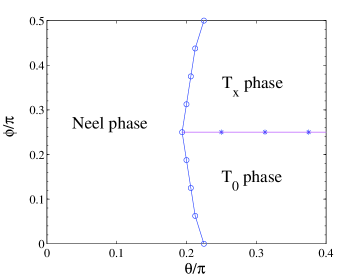
Figure 1: (Color online) The phase diagram of model (I). The transition between the Neel phase and the SPT phases are second order, and the transition between $T_{0}$ and $T_{x}$ is first order.

In this paper, we will study the SPT phases of a spin-chain protected by translational symmetry and on-site $D_{2h}=D_{2}\otimes Z_{2}$ symmetry, where the $Z_{2}$ in $D_{2}\otimes Z_{2}$ is generated by the time reversal symmetry $T$. Here we assume that the physical spin forms a linear representation of $D_{2}$ and $T^{2}=1$. First, we study a simple spin-1 model with those symmetries

$$H = \sum_{i}\Big{[}\cos\theta S_{x,i}S_{x,i+1}+\sin\theta[\cos\phi(S_{y,i}S_{y,i+1}$$

$$+S_{z,i}S_{z,i+1})+\sin\phi(S_{xz,i}S_{xz,i+1}+S_{xy,i}S_{xy,i+1})]\Big{]}.$$

where $S_{mn}=S_{m}S_{n}+S_{n}S_{m}$ $(m,n=x,y,z)$. As shown in Fig. 1, this model has three phases, the Neel phase, the $T_{0}$ phase and the $T_{x}$ phase. The Neel phase breaks the $D_{2h}$ symmetry, and the other two phases do not break any symmetry. We can use sublattice spin magnetization as an order parameter to distinguish the Neel phase. However, the remaining two phases cannot be distinguished through local order parameter such as sublattice spin magnetization. Further, in the both phases, the entanglement spectrumentanglspect is doubly degenerate, so both of them are nontrivial. However, the entanglement spectrum is not a good order parameter to separate them. Therefore, we need a new tool to distinguish these two non-trivial phases that cannot be described by symmetry breaking and the entanglement spectrum. It turns out that the new tool is the projective representation of the symmetry group. The two phases can be distinguished since their doubly degenerate end states form different projective representations of $D_{2h}$. The physical consequence is that they response differently to weak external magnetic field. The doubly degenerate end states can be viewed as an effective spin-1/2 spin with asymmetric $g$-factors: $g_{x}$ and $g_{y}$ and $g_{z}$ describing the coupling of the end spin to external magnetic field in $x$, $y$ and $z$ directions. We find that $g_{x},g_{y},g_{z}\neq 0$ in the $T_{0}$-phase and $g_{x}\neq 0,g_{y}=g_{z}=0$ in the $T_{x}$-phase. We would like to stress that such a property is robust against any perturbations that do not break the $D_{2h}$ symmetry (the perturbation may even break the translation symmetry).

The $D_{2h}$ symmetric spin-chain can have very rich quantum phases. It is shown that it can have $64$ different gapped phases that do not break the $D_{2h}$ and the translation symmetry.CGW3 In fact, it is the projective representation theory that allow one to find all the non-trivial SPT phases beyond the symmetry breaking description. In this paper, we will not study all of them. We will only use 8 classes of projective representations of the $D_{2h}$ group to construct 8 gapped no-symmetry-breaking phases, one is trivial and the other 7 are nontrivial SPT phases. We find that four of the 7 SPT phases (labeled as $T_{0},T_{x},T_{y}$ and $T_{z}$) can be realized in $S=1$ spin chain. Here $T_{0}$ is the usual Haldane phase (because it includes the Heisenberg point), and $T_{x},T_{y},T_{z}$ are new SPT phases. The states in different SPT phases cannot be smoothly connected to each other without explicitly breaking the $D_{2h}$ symmetry in the Hamiltonian. The remaining three SPT phases cannot be realized for $S=1$ chains, but they may exist in $S=1$ spin ladders or $S=2$ spin chains.

The four SPT phases are experimentally distinguishable due to the different behaviors of their end states. In the $T_{0}$ phase, the end states can be considered as spin-1/2 free spins. So weak magnetic field couples to the end spins and lifts the ground state degeneracy at linear order. However, in $T_{x}$ phase, the end states can no longer be considered as normal spin-1/2 spins because they behave differently under time reversal. As mentioned above, the $g$-factors $g_{y},g_{z}\approx 0$, which means that $B_{y}$ and $B_{z}$ can not split the degenerate ground states in $T_{x}$ phase at linear order. Similarly, the end states of $T_{y}$ (or $T_{z}$) only respond to $B_{y}$ (or $B_{z}$). According to these properties, we propose an experimental scenario to distinguish these four phases.

This paper is organized as the following. In section II, we introduce the four SPT phases for the $S=1$ spin chain models. In section III, we focus on the interaction of the end states to weak external magnetic fields and propose an experimental method to distinguish different SPT phases. In section IV we briefly summarize the relationship between the SPT phases and the classes of projective representations, and leave detailed derivations to the appendix. Section V is devoted to conclusions and discussions.

II The model and SPT phases

$D_{2h}$ group has eight group elements, $D_{2h}=\{E,R_{x},R_{y},R_{z},T,R_{x}T,R_{y}T,R_{z}T\}$, which is a direct product of the 180^∘ spin rotation group $D_{2}=\{E,R_{x}=e^{-i\pi S_{x}},R_{y}=e^{-i\pi S_{y}},R_{z}=e^{-i\pi S_{z}}\}$ and time reversal symmetry group $Z_{2}=\{E,T\}$. Note that $T$ inverts the spin $(S_{x},S_{y},S_{z})\to(-S_{x},-S_{y},-S_{z})$ and is anti-unitary. $D_{2h}$ has eight 1-d linear representations (as shown in Tab. 6 in appendix B). Since $T$ is anti-unitary, the bases $|\phi\rangle$ and $i|\phi\rangle$ have different time reversal parity. This subtle property yields more than one SPT phases.

The most general Hamiltonian for an $S=1$ spin chain with $D_{2h}$ symmetry and with only nearest neighbor interaction is given by

$$H_{D_{2h}} = \sum_{i}[a_{1}S_{x,i}^{2}S_{x,j}^{2}+a_{2}(S_{x,i}^{2}S_{y,j}^{2}+S_{y,i}^{2}S_{x,j}^{2})$$ (2)

$$+a_{3}S_{y,i}^{2}S_{y,j}^{2}+a_{4}(S_{x,i}^{2}S_{z,j}^{2}+S_{z,i}^{2}S_{x,j}^{2})$$

$$+a_{5}S_{z,i}^{2}S_{z,j}^{2}+a_{6}(S_{y,i}^{2}S_{z,j}^{2}+S_{z,i}^{2}S_{y,j}^{2})$$

$$+b_{1}S_{x,i}S_{x,j}+b_{2}S_{yz,i}S_{yz,j}+c_{1}S_{y,i}S_{y,j}$$

$$+c_{2}S_{xz,i}S_{xz,j}+d_{1}S_{z,i}S_{z,j}+d_{2}S_{xy,i}S_{xy,j}$$

$$+e_{1}S_{x,i}^{2}+e_{2}S_{y,i}^{2}+e_{3}S_{z,i}^{2}].$$

where $j=i+1$, $S_{mn}=S_{m}S_{n}+S_{n}S_{m}$ $(m,n=x,y,z)$ and $a_{1},a_{2},...,e_{1},e_{2},e_{3}$ are constants. We are interested in the parameter regions within which the excitations are gapped and the ground states respect the $D_{2h}$ symmetry.

In general, for 1D systems with translation symmetry and on-site symmetry group $G$, a gapped ground state that does not break any symmetry can be approximately written as a matrix product state (MPS)

$$|\psi\rangle=\sum_{\{m_{1},...,m_{N}\}}\mathrm{Tr}(A^{m_{1}}...A^{m_{N}})|m_{1}...m_{N}\rangle,$$ (3)

which varies in the following way under the symmetry group

$$\sum_{m^{\prime}}u(g)_{mm^{\prime}}A^{m^{\prime}}=\alpha(g)M(g)^{\dagger}A^{m}M(g)$$ (4)

where $g\in G$ is a group element, and $\alpha(g)$/$M(g)$ is its linear/projective representation matrix. Thus it is concluded that the SPT phases are classified by $(\omega,\alpha)$, where $\omega$ is the element of the second cohomology group $H^{2}(G,\mathbb{C})$ (which describe different classes of projective representations of the symmetry group $G$).CGW2

So in our case, the ground state can be generally written in forms of MPS shown in Eq. (3). The requirement $|\psi\rangle$ being invariant under $D_{2h}$ is equivalent to the condition in Eq. (4). The main task of this paper is to try to find different kinds of states that satisfy this condition. In this paper, we only consider the case $\alpha(g)=1$. The full classification (with a different approach from this paper) is given in Ref. CGW3, .

Let us first consider the on-site terms in (2). When $|e_{1}|$, $|e_{2}|$ or $|e_{3}|$ is large, the ground state of $H_{D_{2h}}$ is simple. For instance, when $e_{3}\to-\infty$, the ground state is a long-range ordered state which breaks the $D_{2h}$ symmetry; when $e_{3}\to\infty$, the ground state is a product state $|\psi\rangle=\prod_{i}\otimes|0\rangle_{i}$, which is trivial.e1e2e3 Since we are interested in the nontrivial SPT phases, we will set $e_{1}=e_{2}=e_{3}=0$ in the following discussion.

II.1 Exactly solvable models

The Affleck Kennedy Lieb Tasaki (AKLT) modelAKLT is an exactly solvable model with $SO(3)$ symmetry that falls in the Haldane phase. The AKLT model contains all the physical properties of the Haldane phase and all other states in this phase can smoothly deform into the AKLT state. Since the ground state wave function of this exactly solvable model is a simple matrix product (sMP) stateiMPS and is known in advance, so studying this model is relatively easy and helps to understand the physics of the Haldane phase.

In this section, we will introduce four classes of exactly solvable models that have $D_{2h}$ symmetry. Analogous to the AKLT state, the ground states of these exactly solvable models are nontrivial sMP states satisfying Eq. (4). We will show that different classes of sMP states can not be smoothly connected, which indicates that each class corresponds to a phase.

The first example is a direct generalization of the AKLT model. The ground state of AKLT state is represented by $A^{x}=\sigma_{x},\ A^{y}=\sigma_{y},\ A^{z}=\sigma_{z}$, which has $SO(3)$ symmetry. When generalized to $D_{2h}$ symmetry, we obtain

$$A^{x}=a\sigma_{x},\ \ A^{y}=b\sigma_{y},\ \ A^{z}=c\sigma_{z},$$ (5)

where $a,b,c$ are nonzero real numbers (the same below). When $a=b=c=1$, the above state reduces to the AKLT state. For this reason, we say that this model also belongs to the Haldane phase. We label this phase as $T_{0}$. Similar to the AKLT model, the parent Hamiltonian of above state is composed by projectors (for details see appendix A and B)

$$H_{0} = \sum_{i}\left[({1\over 4}+b^{2}c^{2}\gamma)S_{x,i}S_{x,j}+({1\over 4}+a^{2}c^{2}\gamma)S_{y,i}S_{y,j}\right.$$ (6)

$$\left.+({1\over 4}+a^{2}b^{2}\gamma)S_{z,i}S_{z,j}+({1\over 4}-{b^{2}c^{2}\gamma})S_{yz,i}S_{yz,j}\right.$$

$$\left.+({1\over 4}-{a^{2}c^{2}\gamma})S_{xz,i}S_{xz,j}+({1\over 4}-{a^{2}b^{2}\gamma})S_{xy,i}S_{xy,j}\right]$$

$$\left.\right.+h_{0}.$$

where $\gamma={1\over 2(a^{4}+b^{4}+c^{4})}$ and

$$h_{0} = -\sum_{i}[c^{4}{\gamma}(S_{x,i}^{2}S_{y,j}^{2}+S_{y,i}^{2}S_{x,j}^{2})+{b^{4}\gamma}(S_{x,i}^{2}S_{z,j}^{2}$$

$$+S_{z,i}^{2}S_{x,j}^{2})+{a^{4}\gamma}(S_{y,i}^{2}S_{z,j}^{2}+S_{z,i}^{2}S_{y,j}^{2})].$$

At open boundary condition, the Hamiltonian (6) has exactly four-fold degenerate ground states independent of the chain length. The above exactly solvable model is frustration free, that is, the expectation value of the Hamiltonian is minimized locally in the ground states. The excitations are gapped and all correlation functions of local operators are short ranged. Furthermore, if $a,b,c$ are normalized $a^{2}+b^{2}+c^{2}=1$, then it is easily checked that

$$\sum_{m}A^{m}(A^{m})^{\dagger}=I,\ \ \sum_{m}(A^{m})^{\dagger}\Lambda^{2}A^{m}=\Lambda^{2},$$

here $\Lambda=I$, indicating that the entanglement spectrum of the ground states is doubly degenerate. This informs that state (5) is nontrivial. Actually, the models at the vicinity of (6) (the phase $T_{0}$) have very similar properties unless gap closing (second order phase transition) or level crossing (first order phase transition) happens.

Now we consider another example of sMP state,

$$A^{x}=ia\sigma_{x},\ \ A^{y}=b\sigma_{y},\ \ A^{z}=c\sigma_{z}.$$ (7)

Above sMP state is also invariant under $D_{2h}$ group. As will be shown later, it can not be continuously connected to Eq. (5) without breaking the $D_{2h}$ symmetry. This means that it belongs to another phase which we label as $T_{x}$ phase. The parent Hamiltonian of (7) is given by

$$H_{x} = \sum_{i}\left[({1\over 4}+b^{2}c^{2}\gamma)S_{x,i}S_{x,j}+({1\over 4}-a^{2}c^{2}\gamma)S_{y,i}S_{y,j}\right.$$ (8)

$$\left.+({1\over 4}-a^{2}b^{2}\gamma)S_{z,i}S_{z,j}+({1\over 4}-{b^{2}c^{2}\gamma})S_{yz,i}S_{yz,j}\right.$$

$$\left.+({1\over 4}+{a^{2}c^{2}\gamma})S_{xz,i}S_{xz,j}+({1\over 4}+{a^{2}b^{2}\gamma})S_{xy,i}S_{xy,j}\right]$$

$$\left.\right.+h_{0}.$$

Similarly, the third example

$$A^{x}=a\sigma_{x},\ \ A^{y}=ib\sigma_{y},\ \ A^{z}=c\sigma_{z}$$ (9)

belongs to the $T_{y}$ phase and its parent Hamiltonian is

$$H_{y} = \sum_{i}\left[({1\over 4}-b^{2}c^{2}\gamma)S_{x,i}S_{x,j}+({1\over 4}+a^{2}c^{2}\gamma)S_{y,i}S_{y,j}\right.$$ (10)

$$\left.+({1\over 4}-a^{2}b^{2}\gamma)S_{z,i}S_{z,j}+({1\over 4}+{b^{2}c^{2}\gamma})S_{yz,i}S_{yz,j}\right.$$

$$\left.+({1\over 4}-{a^{2}c^{2}\gamma})S_{xz,i}S_{xz,j}+({1\over 4}+{a^{2}b^{2}\gamma})S_{xy,i}S_{xy,j}\right]$$

$$\left.\right.+h_{0}.$$

The last example

$$A^{x}=a\sigma_{x},\ \ A^{y}=b\sigma_{y},\ \ A^{z}=ic\sigma_{z}$$ (11)

belongs to the $T_{z}$ phase with its parent Hamiltonian given by

$$H_{z} = \sum_{i}\left[({1\over 4}-b^{2}c^{2}\gamma)S_{x,i}S_{x,j}+({1\over 4}-a^{2}c^{2}\gamma)S_{y,i}S_{y,j}\right.$$ (12)

$$\left.+({1\over 4}+a^{2}b^{2}\gamma)S_{z,i}S_{z,j}+({1\over 4}+{b^{2}c^{2}\gamma})S_{yz,i}S_{yz,j}\right.$$

$$\left.+({1\over 4}+{a^{2}c^{2}\gamma})S_{xz,i}S_{xz,j}+({1\over 4}-{a^{2}b^{2}\gamma})S_{xy,i}S_{xy,j}\right]$$

$$\left.\right.+h_{0}.$$

Above we have given four special models that belong to different SPT phases. In the next subsection, we will show that if one keeps the $D_{2h}$ symmetry, phase transitions must happen when connecting these models.

II.2 transitions between different SPT phases

In order to justify the four SPT phase, we will use numerical method to study more general Hamiltonians. The method we adopt is one version of the tensor renormalization group approach developed in 1D by G. VidalVidal and later generalized to 2D by T. Xiang et.al.TensRG In this method, the ground state is approximated by a MPS. For an arbitrarily initialized state, we can act the (infinitesimal) imaginary time evolution operator $U(\delta\tau)=e^{-H\delta\tau}$ for infinite times, finally obtaining the fixed point matrix $A^{m}$. If the dimension $D$ of $A^{m}$ is not too small, the corresponding MPS is very close to the true ground state. In our numerical calculation, we set $D=16$. In 1D, the ground state energy, correlation functions, density matrix, and entanglement spectrum can be calculated directly from the matrix $A^{m}$.

Noticing that $h_{0}$ is a common term in the four exactly solvable models, which indicates that it is unimportant and can be dropped. This can be numerically verified. For this purpose, we add a perturbation to the models, such as (8),

$$H(\eta)=H_{x}-\eta h_{0},$$ (13)

where $\eta\in[0,1]$. As shown in Fig. 2, the ground state energy $E(\eta)$ and its derivatives $E^{\prime}(\eta),E^{\prime\prime}(\eta)$ are all smooth functions, indicating that all the Hamiltonians $H(\eta)$ belong to the same phase. Using the same method, one can also check that the Hamiltonians (with $D_{2h}$ symmetry) in the vicinity of an exactly solvable model fall in the same phase. For instance, the Heisenberg model and $H_{0}$ in (6) are in the same phase.

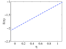
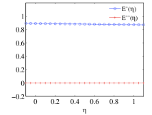
Figure 2: (Color online) (a) The energy curve $E(\eta)$, (b) The first and second derivatives of $E(\eta)$. All these curves are smooth, indicating that these states are in the same phase.

Now a question is whether the ground states of different exactly solvable models can be smoothly transformed into each other. For this end, we consider a more realistic model (I) which connects two exactly solvable models, such as $H_{0}$ and $H_{x}$. We are interested in the anti-ferromagnetic cases and will focus on the parameter region $\theta,\phi\in[0,{\pi\over 2}]$. The point $({\pi\over 4},0)$ is the Heisenberg model. From the result of the last paragraph, the Heisenberg model is in the same phase as (6), and similarly $({\pi\over 4},{\pi\over 2})$ is in the same phase as (8). If these two points cannot be smoothly connected (i.e.,if gap closing or level crossing will unavoidably happen), then (6) and (8) belong to different phases.

Using the tensor RG method, we can calculate the ground state energy of (I) and the phase diagram is shown in Fig. 1. When $\theta$ is less then ${0.21\pi}$, the ground state is Neel ordered. When $\theta$ increases, a second order phase transition occurs and we enter the SPT phases. Fig. 3 shows the data of energy curve with fixed $\phi={\pi\over 8}$ (and $\phi={3\pi\over 8}$) and its first and second derivatives , which illustrate this transition.

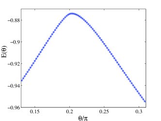
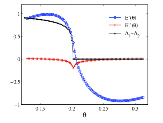
Figure 3: (Color online) (a) The energy curve $E(\theta)$ with fixed $\phi={\pi\over 8}$ (and $\phi={3\pi\over 8}$ ). (b) The line with circles is the first order derivative and the line with crosses is the second order derivative of $E(\theta)$; the doted line is the difference tween the two biggest weights of the entanglement spectrum $\Lambda_{1}-\Lambda_{2}$. Since $E^{\prime}(\theta)$ is continuous but $E^{\prime\prime}(\theta)$ is not, the transition is second order. The degeneracy of $\Lambda_{1}$ and $\Lambda_{2}$ indicates that the $T_{0}$ (and $T_{x}$) phase is nontrivial.

The region $\phi\in[0,{\pi\over 4})$ belongs to the $T_{0}$ phase and $\phi\in({\pi\over 4},{\pi\over 2}]$ belongs to the $T_{x}$ phase. A first order phase transition between them happens at $\phi={\pi\over 4}$.

The first order phase transition occurs exactly at $\phi={\pi\over 4}$. This is because the whole phase diagram is symmetric above and below the line $\phi={\pi\over 4}$. This symmetry can be seen in the Hamiltonian. Notice that under a unitary matrix $U$, we get

$$U^{\dagger}S_{x}U=S_{x},\ \ U^{\dagger}S_{y}U=-S_{xz},\ \ U^{\dagger}S_{z}U=S_{xy},$$ (14)

where $U=\left(\begin{matrix}{1\over\sqrt{2}}e^{i{\pi\over 4}}&0&{1\over\sqrt{2}}e^{-i{\pi\over 4}}\\ 0&1&0\\ {1\over\sqrt{2}}e^{-i{\pi\over 4}}&0&{1\over\sqrt{2}}e^{i{\pi\over 4}}\end{matrix}\right)$. SU(2) This means that Hamiltonian (I) satisfies $(\prod_{i}\otimes U_{i})^{\dagger}H(\theta,\phi)(\prod_{i}\otimes U_{i})=H(\theta,{\pi\over 2}-\phi)$, which yields $E(\theta,\phi)=E(\theta,{\pi\over 2}-\phi)$, and their ground states are transformed by the (local) unitary transformation $\prod_{i}\otimes U_{i}$. But this unitary transformation is not invariant under time reversal $T$, so the behavior of the ground state also changes under time reversal. Resultantly, the state after the transformation belongs to a different phase.

The entanglement spectrum of the ground states can also be obtained programmatically. We find that in both $T_{0}$ and $T_{x}$ phases the entanglement spectrum is doubly degenerate (see Fig. 3). This shows that the $T_{0}$ and $T_{x}$ phases are indeed nontrivial. Similar to the model (I), the phase transition between $T_{0}$ and $T_{y}$ or between $T_{0}$ and $T_{z}$ can also be illustrated.

Now we will show that first order phase transition also exists between any two of $T_{x},T_{y},T_{z}$. As an example, we consider the model that contains the transition between $T_{x}$ and $T_{z}$ phases:

$$H = \sum_{i}[{1\over 6}S_{y,i}S_{y,j}+{5\over 6}S_{xz,i}S_{xz,j}+\cos\theta(S_{x,i}S_{x,j}$$

$$+S_{xy,i}S_{xy,j})+\sin\theta(S_{z,i}S_{z,j}+S_{yz,i}S_{yz,j})].$$

When $\theta=\tan^{-1}{1\over 5}$, the above Hamiltonian is in the same phase as $H_{x}$ as shown in (13), and when $\theta=\tan^{-1}5$, it is in the same phase as $H_{z}$. The ground state energy of (II.2) as a function of $\theta$ can be obtained using the tensor RG method, and the result is shown in Fig. 4. A first order transition at $\theta={\pi\over 4}$ manifests itself. For the reason similar to (14), the model also has a symmetry $E(\theta)=E({\pi\over 2}-\theta)$.

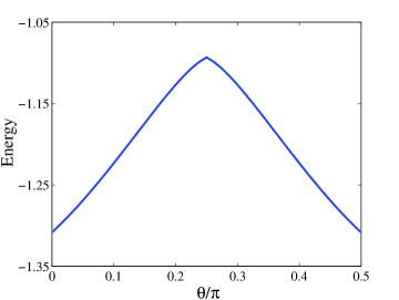
Figure 4: (Color online) The ground state energy for model (II.2). A first order phase transition is obvious.

From the above analysis, we can conclude that the four exactly solvable models really stand for four distinct SPT phases. All these SPT phases are protected by the $D_{2h}$ symmetry. As will be shown in section IV, no more SPT phases exist for $S=1$ models with $D_{2h}$ symmetry. Furthermore, the Eqs. (I) and (II.2) show that these SPT phases can be obtained by much simpler Hamiltonians which is hopefully realized experimentally.

Now an interesting question arises, how to distinguish these SPT phases in a practical way? It is impossible to distinguish these phases by linear response in the bulk since it is gapped. However, the end ‘spins’ localized at open boundaries may have different behaviors in different SPT phases. In the next section, we will propose an experimental method to detect each SPT phase.

III Distinguishing different SPT phases

We expect to distinguish the four SPT phases through their different physical properties. Experimentally, all measurable physical quantities are response functions, or susceptibilities. So we need to add small perturbations and expect that (the ‘end spins’ of) different phases have different responses. The simplest perturbation for spin system is magnetic field $H^{\prime}=g_{L}\mu_{B}\mathbf{B}\cdot\tilde{\mathbf{S}}$, here $\tilde{\mathbf{S}}=\sum_{i}\mathbf{S}_{i}$, $g_{L}$ is the Lande factor and $\mu_{B}$ is the Bohr magneton. We will study the linear response to small $\mathbf{B}$.

Since the states in the same phase have the same universal properties, we will focus on the exactly solvable models first. For simplicity, we consider the AKLT model, namely, $H_{0}$ with $a=b=c=1$. In the matrix product state picture, the physical $S=1$ spin is divided into two $J=1/2$ virtual spins. In the AKLT state, the virtual spins pair into singlets (called valence bonds) on each link between neighboring sites. Under open boundary condition, a free $J=1/2$ spin at each end remains unpaired. The two end spins account for the exactly four-fold degeneracy of the ground states. In this picture, it’s easy to calculate the total spin in the ground state Hilbert space. The singlets in the bulk have no contributions to $\tilde{\mathbf{S}}$, only the two end spins $\mathbf{j}_{1}$ and $\mathbf{j}_{2}$ contribute and resultantly $\tilde{\mathbf{S}}=\mathbf{j}_{1}+\mathbf{j}_{2}$. In this sense, the end spins can be considered as impurity spins of a paramagnetic material. Since the total spin of an open chain is ${1\over 2}\otimes{1\over 2}=0\oplus 1$, we expect that the eigenvalue of $\tilde{S}_{x},\tilde{S}_{y},\tilde{S}_{z}$ should be $1,-1,0,0$. This can be verified by exact diagonalizing a short chain. We denote these four degenerate ground states as $|\psi_{1}\rangle,|\psi_{2}\rangle,|\psi_{3}\rangle,|\psi_{4}\rangle$. Then the matrix element of $\tilde{S}_{m}$ in the ground state Hilbert space is given by

$$\tilde{S}_{m}^{\alpha\beta}=\langle\psi_{\alpha}|\tilde{S}_{m}|\psi_{\beta}\rangle,\ \ \alpha,\beta=1,2,3,4$$ (16)

The eigenvalues of the matrices $(\tilde{\mathbf{S}}^{\alpha\beta})$ are exactly $1,-1,0,0$ and these values are independent of the length of the chain. Thus a small magnetic field along any direction $H^{\prime}=g_{L}\mu_{B}B_{x}S_{x}$ or $g_{L}\mu_{B}B_{y}S_{y}$ or $g_{L}\mu_{B}B_{z}S_{z}$ will split the ground state degeneracy and give rise to a finite magnetization.

At finite temperature, the susceptibility satisfies the Curie law and is given byKittle

$$\chi(T)\simeq{Ng^{2}\mu_{B}^{2}\over 3k_{B}T},$$ (17)

where $N$ is the number of end spins, $g=\sqrt{J(J+1)}g_{L}$, $J=1/2$ and $g_{L}$ is the Lande $g$ factor. If the spin-1 chains in the sample are broken into long separate segments, then $N$ can be a considerable number. We also note that, in real samples, the susceptibility also contains a temperature independent part coming from the bulk.

We see that, for the AKLT model, the spin susceptibility diverges at low temperature along all directions. For a general model in the $T_{0}$ phase, the divergence of $\chi_{x}(T),\chi_{y}(T),\chi_{z}(T)$ still holds, except that it is no longer isotropic.

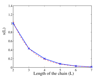
Figure 5: (Color online) The eigenvalues of $\tilde{S}_{y}$ and $\tilde{S}_{z}$ are $s,-s,0,0$. The magnitude of $s$ exponentially decays with the length of the chain in $T_{x}$ phase. The dashed line is an exponential fit. The results are obtained by exact diagonalization and we only calculate up to seven sites.

However, in phase $T_{x}$, the end ‘spins’ have absolutely different physical properties. We consider the model $H_{x}$ in (8), and set $a=b=c=1$. Then we calculate the eigenvalues of operators $\tilde{S}_{x},\tilde{S}_{y}$ and $\tilde{S}_{z}$ in the ground state Hilbert space as before. We find that the eigenvalues of $(\tilde{S}^{\alpha\beta})_{x}$ are still $1,-1,0,0$, meaning that along $x$ direction the spin-1/2 end spins still exist and $\chi_{x}(T)$ diverges at $T=0$. The eigenvalues of $(\tilde{S}^{\alpha\beta})_{y}$ and $(\tilde{S}^{\alpha\beta})_{z}$ also have the structure $s,-s,0,0$, but the magnitude of the nonzero eigenvalues $s$ exponentially decay to zero with the increasing of the length of the chain (see Fig. 5). This means that in $y$- and $z$-directions, there are no free spins coupled to the magnetic field. In appendix D we will show that this property is determined by the projective representation carried by the virtual ‘spins’. In this case, $\chi_{y}(T)$ and $\chi_{z}(T)$ are given by (17) with $g_{y},g_{z}\approx 0$. The result that $\chi_{x}(T)$ follows Curie law and $\chi_{y}(T)$, $\chi_{z}(T)$ has effective $g_{y},g_{z}\approx 0$ is a universal property of all the models in the $T_{x}$ phase.

Similarly, one can check that only $\chi_{y}(T)$ follows Curie law in $T_{y}$ phase with the usual $g_{y}\approx\sqrt{J(J+1)}g_{L}$ ($g_{x},g_{z}\approx 0$), and similarly only $\chi_{z}(T)$ follows Curie law in $T_{z}$ phase with the usual $g_{z}\approx\sqrt{J(J+1)}g_{L}$ ($g_{x},g_{y}\approx 0$). Therefore, by measuring the temperature dependence of susceptibility and the effective $g$ in $x,y,z$ directions, we are able to distinguish the four SPT phases.

IV projective representations and SPT phases

In previous sections, we have given four SPT phases of the model (2) and studied their physical properties. In this section, we will explain how the $D_{2h}$ symmetry supports the existence of these phases. Then we will discuss other possible SPT phases of spin systems with $D_{2h}$ symmetry.

The ground state of a gapped phase is written as (3). If we require that the ground state MPS be invariant under the symmetry group $D_{2h}$, namely, $g|\psi\rangle=|\psi\rangle$ ($g\in D_{2h}$), then under the action of the symmetry group the matrix $A^{m}$ must vary in the following way.

1) $g$ is unitary, $g\in\{E,R_{x},R_{y},R_{z}\}$,

$$\sum_{m^{\prime}}u(g)_{mm^{\prime}}A^{m^{\prime}}=M(g)^{\dagger}A^{m}M(g);$$ (18)

2) $g$ is anti-unitary, $g\in\{T,R_{x}T,R_{y}T,R_{z}T\}$,

$$\sum_{m^{\prime}}u(g)_{mm^{\prime}}KA^{m^{\prime}}=M(g)^{\dagger}A^{m}M(g).$$ (19)

Here $u(g)$ and $M(g)$ are representations of the symmetry group $D_{2h}$. The matrices $u(g)$ satisfy the same multiplication law of $D_{2h}$ group and is called a linear representation. The physical spin freedoms are linear representations of $D_{2h}$. $M(g)$ and $M(g)e^{i\theta}$ are equivalent and belong to the same presentation. Up to a phase factor (which depends on the group elements), $M(g)$ satisfy the multiplication law of $D_{2h}$, and this kind of presentation is called a projective representation. The virtual ‘spins’ (and the end states) are projective representations of $D_{2h}$. More knowledge about projective representation can be found in Ref. CGW2, ; Boyal, .

The $D_{2h}$ group has eight 1-d linear representations (see Tab. 6) and eight (and only eight) classes of projective representations labeled by (111), (11-1),(1-11),(1-1-1),(-111),(-11-1),(-1-11) and (-1-1-1) (see Tab. 7). The first class of projective representation (111) is the eight 1-d linear representations, which are trivial (an example of the the corresponding trivial phase is the case $e_{3}\to\infty$). The other seven projective representations are 2-d and nontrivial. Since states supporting different projective representations (or virtual ‘spins’) cannot be smoothly transformed into each other, each projective representation corresponds to a SPT phase. This means that there should be at least seven different nontrivial SPT phases for spin systems respecting $D_{2h}$ symmetry. (In fact, when considering different $\alpha(g)$ there are more nontrivial SPT phases for spin systems respecting $D_{2h}$ symmetry.CGW3 )

How can we obtain the projective representations? Mathematically, finding the projective representations of a group $G$ is equivalent to find the linear representations of its cover group, which is a central extension of $G$ and is called representation group $R(G)$. Boyal The representation group $R(D_{2h})$ is available in literature, Boyal so we can calculate the matrix elements of all the projective representations of $D_{2h}$ (see Tab. 7).

Once the matrices of the projective representations are obtained, we can calculate the CG coefficients for decomposing the direct product of two projective representations. From the CG coefficients, we can construct sMP states and their parent Hamiltonians.Tu The models (6),(8),(10) and (12) are constructed accordingly and correspond to the (-1-1-1),(-1-11),(-11-1),(-111) representations respectively. From these models we can know what kind of interactions are essential for each SPT phase.

As shown in appendix B, the remaining three SPT phases of (1-11),(11-1),(1-1-1) cannot be realized for $S=1$ spin chains. The reason is that the physical freedom is not sufficient to support the direct product of two such projective representations. However, these phases might be realized in $S=1$ spin ladders or $S=2$ models, and this will be our upcoming work.

V conclusion and discussion

In summary, we have found four nontrivial SPT phases $T_{0},T_{x},T_{y},T_{z}$ of $S=1$ spin chains which have on-site $D_{2h}$ symmetry. These SPT phases have similar properties as the usual Haldane phase, such as the bulk excitation gap, short-range correlations, existence of end ‘spins’, entanglement spectrum degeneracy. However, the different projective representations of the end spin under $D_{2h}$ indicate that they do belong to different phases. The SPT order that distinguishes them is the class of projective representations (or the group elements of the second cohomology $H^{2}(D_{2h},\mathbb{C})$) correspond to the ground states (or the matrices $A^{m}$).

We find that different SPT phases can be distinguished by experimental method. The magnetic susceptibilities $\chi_{x},\chi_{y},\chi_{z}$ obey Curie law and diverge at zero temperature. In $T_{0}$ phase the effective $g$-factors of the end spin have the usual values for magnetic field in $x$-, $y$-, and $z$-directions. But in $T_{x}$ (or $T_{y}$ or $T_{z}$) phase, the effective $g\approx\sqrt{J(J+1)}g_{L}$ has the usual value only for magnetic field in $x$-direction (or $y$-direction or $z$-direction). The effective $g\approx 0$ [see eq. (17)] for magnetic field in the other two directions.

From the seven nontrivial projective representations for $D_{2h}$ group, we constructed seven SPT phases. Four of them are discussed above. The other three may be realized in $S=1$ spin ladders or spin $S=2$ models and are not discussed in the current paper. Some conclusion in this paper can be generalized to larger spin systems and higher dimensions.

VI acknowledgements

We thank Xie Chen, Hong-Hao Tu, Zheng-Yu Weng and Hai-Qing Lin for helpful discussions. This research is supported by NSF Grant No. DMR-1005541 and NSFC 11074140.

Appendix A Spin chian with $D_{2}$ symmetry

In appendix A, we will first study $S=1$ spin systems with $D_{2}$ symmetry. The same method can be applied to $D_{2h}$ case.

A.1 General Hamiltonian with $D_{2}$ point group symmetry

The point group $D_{2}$ has only four elements, $D_{2}=\{E,R_{x},R_{y},R_{z}\}$. The multiplication table is shown in Tab. 1.

Table 1: Multiplication table of $D_{2}$

	$E$	$R_{x}$	$R_{y}$	$R_{z}$
$E$	$E$	$R_{x}$	$R_{y}$	$R_{z}$
$R_{x}$	$R_{x}$	$E$	$R_{z}$	$R_{y}$
$R_{y}$	$R_{y}$	$R_{z}$	$E$	$R_{x}$
$R_{z}$	$R_{z}$	$R_{y}$	$R_{x}$	$E$

It has four 1-d linear representations, whose matrix elements and bases of representations are shown in Tab. 2. From quantum mechanics, we know that the $2S+1$ bases of integer spin-$S$ span an irreducible linear representation space of $SO(3)$ group. This Hilbert space is reduced into a direct sum of $2S+1$ 1-d irreducible linear representation spaces of $D_{2}$. For example, when $S=1$ (a vector), the bases

$$|x\rangle={1\over\sqrt{2}}(|-1\rangle-|1\rangle),$$

$$|y\rangle={1\over\sqrt{2}}i(|-1\rangle+|1\rangle),$$

$$|z\rangle=|0\rangle$$

form the $B_{3},B_{2},B_{1}$ representations of $D_{2}$ respectively.

Table 2: Linear representations of $D_{2}$

	$E$	$R_{x}$	$R_{y}$	$R_{z}$		bases or operators
$A$	1	1	1	1	$|0,0\rangle$		$S_{x}^{2},S_{y}^{2},S_{z}^{2}$
$B_{1}$	1	-1	-1	1	$|1,z\rangle$	$S_{z}$	$S_{xy}$
$B_{2}$	1	-1	1	-1	$|1,y\rangle$	$S_{y}$	$S_{xz}$
$B_{3}$	1	1	-1	-1	$|1,x\rangle$	$S_{x}$	$S_{yz}$

Here we focus on the $S=1$ model with nearest neighbor interaction. The general Hamiltonian with $D_{2}$ symmetry is given by

$$H_{D_{2}} = H_{D_{2h}}+f_{1}(S_{x,i}S_{yz,j}+S_{yz,i}S_{x,j})$$ (20)

$$+f_{2}(S_{y,i}S_{xz,j}+S_{xz,i}S_{y,j})$$

$$+f_{3}(S_{z,i}S_{xy,j}+S_{xy,i}S_{z,j}).$$

where $f_{1},f_{2},f_{3}$ are constants and $H_{D_{2h}}$ is given in (2). The above Hamiltonian $H_{D_{2}}$ also has translational symmetry and spacial inversion symmetry. The additional $f_{1},f_{2},f_{3}$ terms are odd under time reversal and break the $T$ symmetry of $H_{D_{2}}$. To study the SPT phases, we need to obtain the projective representations of $D_{2}$.

A.2 Projective representation and CG coefficients of $D_{2}$

From Ref. Boyal, , determining the projective representation of a point group $G$ is equivalent to determining the linear representation of its representation group(s) $R(G)$ (which cover $G$ integer times). There are two non-isomorphism representation groups of $D_{2}$, namely, $R_{1}(D_{2})$ and $R_{2}(D_{2})$, both of which have two generators $P$, $Q$ and eight group elements. Their multiplication tables are listed in Tabs. 3 and 4. In the following, we will mainly discuss the covering group $R_{1}(D_{2})$, and leave the discussion about $R_{2}(D_{2})$ to the end of this section.

Table 3: Multiplication table of $R_{1}(D_{2}$). Notice that $P^{4}=Q^{4}=E$, $P^{2}=Q^{2}$ and $QP=P^{3}Q$.

	$E$	$P^{2}$	$P^{3}$	$P$	$Q$	$P^{2}Q$	$PQ$	$P^{3}Q$
$E$	$E$	$P^{2}$	$P^{3}$	$P$	$Q$	$P^{2}Q$	$PQ$	$P^{3}Q$
$P^{2}$	$P^{2}$	$E$	$P$	$P^{3}$	$P^{2}Q$	$Q$	$P^{3}Q$	$PQ$
$P^{3}$	$P^{3}$	$P$	$P^{2}$	$E$	$P^{3}Q$	$PQ$	$Q$	$P^{2}Q$
$P$	$P$	$P^{3}$	$E$	$P^{2}$	$PQ$	$P^{3}Q$	$P^{2}Q$	$Q$
$Q$	$Q$	$P^{2}Q$	$PQ$	$P^{3}Q$	$P^{2}$	$E$	$P$	$P^{3}$
$P^{2}Q$	$P^{2}Q$	$Q$	$P^{3}Q$	$PQ$	$E$	$P^{2}$	$P^{3}$	$P$
$PQ$	$PQ$	$P^{3}Q$	$P^{2}Q$	$Q$	$P^{3}$	$P$	$P^{2}$	$E$
$P^{3}Q$	$P^{3}Q$	$PQ$	$Q$	$P^{2}Q$	$P$	$P^{3}$	$E$	$P^{2}$

Table 4: Multiplication table of $R_{2}(D_{2})$. Notice that $P^{4}=Q^{2}=E$ and $QP=P^{3}Q$.

	$E$	$P^{2}$	$P^{3}$	$P$	$Q$	$P^{2}Q$	$PQ$	$P^{3}Q$
$E$	$E$	$P^{2}$	$P^{3}$	$P$	$Q$	$P^{2}Q$	$PQ$	$P^{3}Q$
$P^{2}$	$P^{2}$	$E$	$P$	$P^{3}$	$P^{2}Q$	$Q$	$P^{3}Q$	$PQ$
$P^{3}$	$P^{3}$	$P$	$P^{2}$	$E$	$P^{3}Q$	$PQ$	$Q$	$P^{2}Q$
$P$	$P$	$P^{3}$	$E$	$P^{2}$	$PQ$	$P^{3}Q$	$P^{2}Q$	$Q$
$Q$	$Q$	$P^{2}Q$	$PQ$	$P^{3}Q$	$E$	$P^{2}$	$P^{3}$	$P$
$P^{2}Q$	$P^{2}Q$	$Q$	$P^{3}Q$	$PQ$	$P^{2}$	$E$	$P$	$P^{3}$
$PQ$	$PQ$	$P^{3}Q$	$P^{2}Q$	$Q$	$P$	$P^{3}$	$E$	$P^{2}$
$P^{3}Q$	$P^{3}Q$	$PQ$	$Q$	$P^{2}Q$	$P^{3}$	$P$	$P^{2}$	$E$

To obtain all the irreducible representations, we only need to block diagonalize the canonical representation matrices of the two generators $P$ and $Q$. In the canonical representation, the group space itself is also the representation space. Each group element $g_{1}$ is considered as an operator $\hat{g}_{1}$:

$$\hat{g}_{1}(g_{2})=g_{1}g_{2}.$$ (21)

here $g_{2}$ and $g_{1}g_{2}$ are two vectors in the representation space and $\hat{g}_{1}$ becomes a matrix.

The canonical representation matrices of the generators of $R_{1}$ can be read from table 3:

$$P=\left(\begin{matrix}0&0&1&0&0&0&0&0\\ 0&0&0&1&0&0&0&0\\ 0&1&0&0&0&0&0&0\\ 1&0&0&0&0&0&0&0\\ 0&0&0&0&0&0&0&1\\ 0&0&0&0&0&0&1&0\\ 0&0&0&0&1&0&0&0\\ 0&0&0&0&0&1&0&0\end{matrix}\right),Q=\left(\begin{matrix}0&0&0&0&0&1&0&0\\ 0&0&0&0&1&0&0&0\\ 0&0&0&0&0&0&0&1\\ 0&0&0&0&0&0&1&0\\ 1&0&0&0&0&0&0&0\\ 0&1&0&0&0&0&0&0\\ 0&0&1&0&0&0&0&0\\ 0&0&0&1&0&0&0&0\end{matrix}\right),$$

To simultaneously block diagonalize the above matrices, we need to identify the base vectors (or wave function) of each irreducible representation (these base vectors form a unitary matrix which block diagonalize $P$ and $Q$ simultaneously). In quantum mechanics, we use good quantum numbers (eigenvalues of commuting quantities) to label different states. For example, $|S,m\rangle$ symbols a spin state, where $S(S+1)$ is the eigenvalue of the Casimir operator of $SO(3)$ group and $m$ the eigenvalue of the Casimir operator of its subgroup $SO(2)$. Similar method has been applied to the representation theory of groups.ChenJQ What we need to do is to find all the commuting quantities, or the complete set of commuting operators (CSCO).ChenJQ

The Casimir operators of discrete groups are their class operators. For $R_{1}(D_{2})$, there are five classes (hence there are five different irreducible linear representations), and the corresponding five class operators are given as below:

$$C=\{{E},\ {P^{2}},\ {P+P^{3}},\ {Q+P^{2}Q},\ {PQ+P^{3}Q}\}.$$

The class operators commute with each other and all other group elements. This set of class operators $C$ is called CSCO-I in Ref. ChenJQ, . The eigenvalues of the class operators are greatly degenerate, which can only be used to distinguish different irreducible representations(IRs). To distinguish the bases in each IR, we can use the class operators of its subgroup(s). Group $R_{1}$ has a cyclic subgroup

$$C(s)=\{E,P,P^{2},P^{3}\},$$

each element forms a class. The set of class operators of the subgroup is written as $C(s)$. The operator-set $(C,C(s))$ is called CSCO-II, which can be used to distinguish all the bases if every IR occurs only once in the reduced canonical representation.

However, in the reduced canonical representation, a $d$-dimensional representation occurs $d$ times and they have the same eigenvalues for CSCO-II. To lift this degeneracy, we need more commuting operators. Fortunately, we can use the class operators of the ‘intrinsic group’ $\bar{R}_{1}$, whose group elements are defined as follows

$$\hat{\bar{g}}_{1}(g_{2})=g_{2}g_{1}.$$ (22)

Notice that $\hat{\bar{g}}$ commutes with $\hat{g}$ defined in (21). The class operators of $\bar{R}_{1}$ are identical to those of $R_{1}$, $\bar{C}=C$. The set of class operators for the intrinsic subgroup

$$\bar{C}(s)=\{\bar{E},\bar{P},\bar{P}^{2},\bar{P}^{3}\}$$

is noted as $\bar{C}(s)$. The eigenvalues of $\bar{C}(s)$ provide a different set of ‘quantum numbers’ to each identical IR.

Now we obtain the complete set of class operators $\left(C,C(s),\bar{C}(s)\right)$, which is called CSCO-III. The common eigenvectors of the operators in CSCO-III are the orthonormal bases of the irreducible representations, and each eigenvector has a unique ‘quantum number’.

To obtain the bases, we need to simultaneously diagonalize all the operators in CSCO-III and get their eigenvectors. Actually, we only need a few of these operators, for example, we can choose $Q+P^{2}Q$ in $C$, $P$ in $C(s)$ and $\bar{P}$ in $\bar{C}(s)$. The matrices of these operators of $R_{1}(D_{2})$ are given below:

$$Q+P^{2}Q=\left(\begin{matrix}0&0&0&0&1&1&0&0\\ 0&0&0&0&1&1&0&0\\ 0&0&0&0&0&0&1&1\\ 0&0&0&0&0&0&1&1\\ 1&1&0&0&0&0&0&0\\ 1&1&0&0&0&0&0&0\\ 0&0&1&1&0&0&0&0\\ 0&0&1&1&0&0&0&0\end{matrix}\right),$$

$$P=\left(\begin{matrix}0&0&1&0&0&0&0&0\\ 0&0&0&1&0&0&0&0\\ 0&1&0&0&0&0&0&0\\ 1&0&0&0&0&0&0&0\\ 0&0&0&0&0&0&0&1\\ 0&0&0&0&0&0&1&0\\ 0&0&0&0&1&0&0&0\\ 0&0&0&0&0&1&0&0\end{matrix}\right),$$

$$\bar{P}=\left(\begin{matrix}0&0&1&0&0&0&0&0\\ 0&0&0&1&0&0&0&0\\ 0&1&0&0&0&0&0&0\\ 1&0&0&0&0&0&0&0\\ 0&0&0&0&0&0&1&0\\ 0&0&0&0&0&0&0&1\\ 0&0&0&0&0&1&0&0\\ 0&0&0&0&1&0&0&0\end{matrix}\right),$$

Practically, we can diagonalize a linear combination $\hat{O}=(Q+P^{2}Q)+aP+b\bar{P}$, where $a,b$ are arbitrary constants ensuring that all the eigenvalues of $\hat{O}$ are non-degenerate. From the non-degenerate eigenvectors (column vectors) of $\hat{O}$, we obtain an unitary matrix $U$:

$$U=\left(\begin{matrix}{1\over\sqrt{8}}&{1\over\sqrt{8}}&{1\over\sqrt{8}}&{1\over\sqrt{8}}&{1\over 2}&0&0&{1\over 2}\\ {1\over\sqrt{8}}&{1\over\sqrt{8}}&{1\over\sqrt{8}}&{1\over\sqrt{8}}&-{1\over 2}&0&0&-{1\over 2}\\ {1\over\sqrt{8}}&{1\over\sqrt{8}}&-{1\over\sqrt{8}}&-{1\over\sqrt{8}}&-{1\over 2}i&0&0&{1\over 2}i\\ {1\over\sqrt{8}}&{1\over\sqrt{8}}&-{1\over\sqrt{8}}&-{1\over\sqrt{8}}&{1\over 2}i&0&0&-{1\over 2}i\\ {1\over\sqrt{8}}&-{1\over\sqrt{8}}&{1\over\sqrt{8}}&-{1\over\sqrt{8}}&0&-{1\over 2}i&-{1\over 2}i&0\\ {1\over\sqrt{8}}&-{1\over\sqrt{8}}&{1\over\sqrt{8}}&-{1\over\sqrt{8}}&0&{1\over 2}i&{1\over 2}i&0\\ {1\over\sqrt{8}}&-{1\over\sqrt{8}}&-{1\over\sqrt{8}}&{1\over\sqrt{8}}&0&-{1\over 2}&{1\over 2}&0\\ {1\over\sqrt{8}}&-{1\over\sqrt{8}}&-{1\over\sqrt{8}}&{1\over\sqrt{8}}&0&{1\over 2}&-{1\over 2}&0\end{matrix}\right),$$

The matrix $U$ is the transformation that block diagonalizes $P$ and $Q$ simultaneously:

$$U^{\dagger}PU=\left(\begin{matrix}1&0&0&0&0&0&0&0\\ 0&1&0&0&0&0&0&0\\ 0&0&-1&0&0&0&0&0\\ 0&0&0&-1&0&0&0&0\\ 0&0&0&0&-i&0&0&0\\ 0&0&0&0&0&i&0&0\\ 0&0&0&0&0&0&-i&0\\ 0&0&0&0&0&0&0&i\end{matrix}\right),$$ (24)

$$U^{\dagger}QU=\left(\begin{matrix}1&0&0&0&0&0&0&0\\ 0&-1&0&0&0&0&0&0\\ 0&0&1&0&0&0&0&0\\ 0&0&0&-1&0&0&0&0\\ 0&0&0&0&0&i&0&0\\ 0&0&0&0&i&0&0&0\\ 0&0&0&0&0&0&0&i\\ 0&0&0&0&0&0&i&0\end{matrix}\right),$$ (25)

There are four 1-d IRs and one 2-d IR (which occurs twice) in the reduced canonical representation:

$$P_{2}=\left(\begin{matrix}-i&0\\ 0&i\end{matrix}\right)=-i\sigma_{z},Q_{2}=\left(\begin{matrix}0&i\\ i&0\end{matrix}\right)=i\sigma_{x},$$ (26)

So there are totally five independent representations.

The eight elements in $R_{1}$ can be projected onto $D_{2}$, as shown in Tab. 5. And the linear representations of $R_{1}$ correspond to the projective representations of $D_{2}$. The four 1-d IRs correspond to the linear IRs of $D_{2}$, and the 2-d IR stands for a nontrivial projective IR of $D_{2}$. Up to a phase factor, these 2-d matrices are the $180^{\circ}$ rotation operators of a spin with $J=1/2$ (which is a projective IR of SO(3) group).

Table 5: Projection from $R_{1}(D_{2}$) to $D_{2}$

$R_{1}(D_{2})$	$E$	$P$	$Q$	$PQ$
	$P^{2}$	$P^{3}$	$P^{2}Q$	$P^{3}Q$
$D_{2}$	$E$	$R_{z}$	$R_{x}$	$R_{y}$
rotation $\pi$ of $J=1/2$
(up to a phase factor)	$I$	$i\sigma_{z}$	$i\sigma_{x}$	$i\sigma_{y}$

Now let’s look at the direct product of the projective IRs of $D_{2}$. For the 1-d linear IRs, the direct product are still 1-d IRs, which satisfy the following law:

$$A\times B_{1}=B_{1},\ A\times B_{2}=B_{2},\ A\times B_{3}=B_{3},$$

$$B_{1}\times B_{2}=B_{3},\ B_{1}\times B_{3}=B_{2},\ B_{2}\times B_{3}=B_{1}.\$$

The direct product of 1-d and 2-d IRs are still 2-d projective IRs of $D_{2}$. The direct product of two 2-d projective IRs is interesting. It reduces to four 1-d linear IRs. Using the CSCO-II, we can diagonalize the $4\times 4$ matrices $P_{2}\otimes P_{2}$ and $Q_{2}\otimes Q_{2}$ with the following unitary matrix (the column vectors are just the CG coefficients):

$$U_{4}=\left(\begin{matrix}-{1\over\sqrt{2}}&{i\over\sqrt{2}}&0&0\\ 0&0&{1\over\sqrt{2}}&{1\over\sqrt{2}}\\ 0&0&{1\over\sqrt{2}}&-{1\over\sqrt{2}}\\ {1\over\sqrt{2}}&{i\over\sqrt{2}}&0&0\end{matrix}\right),$$

$$U_{4}^{\dagger}(P_{2}\otimes P_{2})U_{4}=\left(\begin{matrix}-1&0&0&0\\ 0&-1&0&0\\ 0&0&1&0\\ 0&0&0&1\end{matrix}\right),$$

$$U_{4}^{\dagger}(Q_{2}\otimes Q_{2})U_{4}=\left(\begin{matrix}1&0&0&0\\ 0&-1&0&0\\ 0&0&-1&0\\ 0&0&0&1\end{matrix}\right),$$

These CG coefficients of the projective IRs of $D_{2}$ are analogous to the decoupling of the direct product of two spins with $J=1/2$, ${1\over 2}\otimes{1\over 2}=1\otimes 0$ except the 3-d IR of spin-1 becomes a direct sum of three 1-d IRS. If we label the bases of the 2-d projective representation of $D_{2}$ as $|\uparrow\rangle,|\downarrow\rangle$, then the CG coefficients are given as:

$$|x\rangle={1\over\sqrt{2}}(|\downarrow_{1}\downarrow_{2}\rangle-|\uparrow_{1}\uparrow_{2}\rangle),$$

$$|y\rangle={i\over\sqrt{2}}(|\downarrow_{1}\downarrow_{2}\rangle+|\uparrow_{1}\uparrow_{2}\rangle),$$

$$|z\rangle={1\over\sqrt{2}}(|\uparrow_{1}\downarrow_{2}\rangle+|\downarrow_{1}\uparrow_{2}\rangle),$$

$$|\mathrm{singlet}\rangle={1\over\sqrt{2}}(|\uparrow_{1}\downarrow_{2}\rangle-|\downarrow_{1}\uparrow_{2}\rangle),$$ (27)

Repeating the above procedure, we obtain the IRs of $R_{2}(D_{2})$. The four 1-d IRs are the same as that of $R_{1}(D_{2})$, while the 2-d IR is given as:

$$P_{2}^{\prime}=\left(\begin{matrix}-i&0\\ 0&i\end{matrix}\right)=-i\sigma_{z},Q_{2}^{\prime}=\left(\begin{matrix}0&1\\ 1&0\end{matrix}\right)=\sigma_{x},$$

The above representation and Eq. (26) differ only by a gauge transformation $P_{2}^{\prime}=P_{2}$ and $Q_{2}^{\prime}=iQ_{2}$, so they belong to the same projective representation of $D_{2}$. The CG coefficients for the 2-d IRs are obtained easily:

$$|x\rangle={1\over\sqrt{2}}(|\downarrow_{1}\downarrow_{2}\rangle+|\uparrow_{1}\uparrow_{2}\rangle),$$

$$|y\rangle={i\over\sqrt{2}}(|\downarrow_{1}\downarrow_{2}\rangle-|\uparrow_{1}\uparrow_{2}\rangle),$$

$$|z\rangle={1\over\sqrt{2}}(|\uparrow_{1}\downarrow_{2}\rangle-|\downarrow_{1}\uparrow_{2}\rangle),$$

$$|\mathrm{singlet}\rangle={1\over\sqrt{2}}(|\uparrow_{1}\downarrow_{2}\rangle+|\downarrow_{1}\uparrow_{2}\rangle).$$ (29)

A.3 sMP state with $D_{2}$ symmetry and its parent Hamiltonian

Before studying the model with $D_{2}$ symmetry, let’s review the $S=1$ AKLT modelAKLT (which has $SO(3)$ symmetry) first. The AKLT state is a sMP state given by $A^{x}=\sigma_{x},A^{y}=\sigma_{y},A^{z}=\sigma_{z}$. The $A^{m}$ matrices are two by two, meaning that the physical spin $S=1$ is viewed as symmetric combination of two $J=1/2$ virtual spins (essentially projective representations of $SO(3)$). Alternatively, we can write the state as

$$|\phi\rangle=\mathrm{Tr}(W_{1}W_{2}...W_{N}),$$ (30)

where $W_{i}=A^{x}|x\rangle_{i}+A^{y}|y\rangle_{i}+A^{z}|z\rangle_{i}$. According to Ref. Tu, , the matrices $A^{m}$ of a sMP state can be obtained by

$$A^{m}=B^{T}(C^{m})^{*},$$ (31)

where $B$ is the CG coefficient combining two virtual spins into a singlet $|\mathrm{0,0}\rangle=B_{m_{1}m_{2}}|{1\over 2},m_{1};{1\over 2},m_{2}\rangle$, and $C^{m}$ is the CG coefficient combining two virtual spins into a triplet $|1,m\rangle=C^{m}_{m_{1}m_{2}}|{1\over 2},m_{1};{1\over 2},m_{2}\rangle$.

Now we can generalize this formalism to the $D_{2}$ case, where the three states of $S=1$ become a direct sum of three IRs of $D_{2}$. $D_{2}$ group has a 2-dimensional nontrivial projective representation, and the direct product of two such projective IRs can be reduced using the CG coefficients ($B$ and $C^{x,y,z}$) in Eq. (A.2). Similar to the $SO(3)$ case, we can consider the two 2-d projective IRs as ‘virtual spins’. From eq. (31), we can construct the following matrix (similar sMP state has been studied in Ref. D2, )

$$W=a\sigma_{x}|x\rangle+b\sigma_{y}|y\rangle+c\sigma_{z}|z\rangle,$$ (32)

where $a,b,c$ are arbitrary nonzero complex constants. The corresponding sMP state is given by $|\phi\rangle=\mathrm{Tr}(W_{1}W_{2}...W_{N})$, which is invariant under the group $D_{2}$. Notice that the CG coefficients in Eq. (A.2) give the same sMP state (up to some gauge transformations). Notice also that (32) is different from (5), (7), (9) or (11). If $a,b$ or $c$ are to be arbitrary complex numbers, it is not invariant under $T$.

The above sMP state is injective, and the parent Hamiltonian can be obtained by projection operators. We consider a block containing two spins, the four matrix elements of $W_{i}W_{i+1}$ span a 4-dimensional Hilbert space. Suppose the orthonormal bases are $|\psi_{1,2,3,4}\rangle_{i}$, then we can construct a projector

$$P_{i}=1-\sum_{\alpha=1}^{4}|\psi_{\alpha}\rangle\langle\psi_{\alpha}|_{i},$$ (33)

and the Hamiltonian $H=\sum_{i}P_{i}$. It can be easily checked that the sMP state is the unique ground state of this Hamiltonian.

The projector $P_{i}$ is a nine by nine matrix that can be written in forms of spin operators. Notice that any Hermitian operator of site $i,j$ can be expanded by the 81 generators of $U(9)=U(3)_{i}\otimes U(3)_{j}$, i.e., $\lambda_{\alpha i}\lambda_{\beta j}$ ($\alpha,\beta=1,...,9$). So, we have

$$P_{i}=\sum_{\alpha,\beta=1}^{9}\xi_{\alpha\beta}\lambda_{\alpha i}\lambda_{\beta j},$$ (34)

where $\xi_{\alpha\beta}$ are constants. Further, the generators of $U(3)$ can be written as polynomials of spin operators.

$$\lambda_{1}=(S_{x}+S_{xz})/\sqrt{2},$$

$$\lambda_{6}=(S_{x}-S_{xz})/\sqrt{2},$$

$$\lambda_{2}=(S_{y}+S_{yz})/\sqrt{2},$$

$$\lambda_{7}=(S_{y}-S_{yz})/\sqrt{2},$$

$$\lambda_{4}=S_{x}^{2}-S_{y}^{2},$$

$$\lambda_{5}=S_{xy},$$

$$\lambda_{3}=(S_{z}+3S_{z}^{2})/2-I,$$

$$\lambda_{8}=(3S_{z}-3S_{z}^{2}+2I)/2\sqrt{3},$$

$$\lambda_{9}=\sqrt{2\over 3}I=\sqrt{1\over 6}(S_{x}^{2}+S_{y}^{2}+S_{z}^{2}).$$

where $S_{mn}=S_{m}S_{n}+S_{n}S_{m},(m,n=x,y,z)$ and $\lambda_{1}\sim\lambda_{8}$ are the Gellmann matrices of $SU(3)$ generators. Finally, we can write the Hamiltonian in forms of spin operators. For simplicity, we first assume $a,b,c$ are real numbers, then the Hamiltonian is given in (6), which is invariant under $T$. The $T$ symmetry goes away when $a,b$ or $c$ becomes an arbitrary complex number. For instance, if $a\to ae^{i\theta}$, then the Hamiltonian (6) becomes

$$H = \sum_{i}\left[({1\over 4}+{b^{2}c^{2}/2\over a^{4}+b^{4}+c^{4}})S_{x,i}S_{x,j}+({1\over 4}+{\cos 2\theta a^{2}c^{2}/2\over a^{4}+b^{4}+c^{4}})S_{y,i}S_{y,j}-{\sin 2\theta{a^{2}c^{2}}/2\over a^{4}+b^{4}+c^{4}}(S_{y,i}S_{xz,j}+S_{xz,i}S_{y,j})\right.$$ (35)

$$\left.+({1\over 4}+{\cos 2\theta a^{2}b^{2}/2\over a^{4}+b^{4}+c^{4}})S_{z,i}S_{z,j}+{\sin 2\theta a^{2}b^{2}/2\over a^{4}+b^{4}+c^{4}}(S_{z,i}S_{xy,j}+S_{xy,i}S_{z,j})+({1\over 4}-{\cos 2\theta a^{2}b^{2}/2\over a^{4}+b^{4}+c^{4}})S_{xy,i}S_{xy,j}\right.$$

$$\left.+({1\over 4}-{b^{2}c^{2}/2\over a^{4}+b^{4}+c^{4}})S_{yz,i}S_{yz,j}+({1\over 4}-{\cos 2\theta a^{2}c^{2}/2\over a^{4}+b^{4}+c^{4}})S_{xz,i}S_{xz,j}\right]+h_{0}$$

When $\sin 2\theta\neq 0$ above Hamiltonian does not have $T$ symmetry.

Varying the values of $a,b,c$, we can transform the ground state of the above Hamiltonian into that of the AKLT model smoothly without breaking $D_{2}$ symmetry. This means that above sMP state also belongs to the Haldane phase. In appendix B we will consider the models with additional time reversal symmetry.

Appendix B Spin Chain with $D_{2h}$ symmetry

In the last section we have studied the spin chain with on-site $D_{2}$ symmetry. Now we consider a $S=1$ spin chain with additional spin-inversion (or time-reversal) symmetry. The complete on-site symmetry now becomes $D_{2h}=\{E,R_{x},R_{y},R_{z},T,R_{x}T,R_{y}T,R_{z}T\}$. It has eight 1-d linear real IRs, as listed in Tab. 6. Notice the time reversal operator $T=e^{-i\pi S_{y}}K$ is anti-unitary, so the states $|m\rangle$ and $i|m\rangle$ ($m=x,y,z$) belong to different linear representations, the former is odd under $T$ and is noted by index $u$, and the latter is even under $T$ as noted by $g$. So we need to introduce six bases $|x\rangle,|y\rangle,|z\rangle$ and $i|x\rangle,i|y\rangle,i|z\rangle$. To construct a sMP state, at least one of the pair $|x\rangle$, $i|x\rangle$ (and also the pairs $|y\rangle$, $i|y\rangle$ and $|z\rangle$, $i|z\rangle$) should be present in the physical bases.

Table 6: Linear representations of $D_{2h}$

	$E$	$R_{x}$	$R_{y}$	$R_{z}$	$T$	$R_{x}T$	$R_{y}T$	$R_{z}T$	bases	operators
$A_{g}$	1	1	1	1	1	1	1	1	$|0,0\rangle$	$S_{x}^{2},S_{y}^{2},S_{z}^{2}$
$B_{1g}$	1	-1	-1	1	1	-1	-1	1	$i|1,z\rangle$	$S_{xy}$
$B_{2g}$	1	-1	1	-1	1	-1	1	-1	$i|1,y\rangle$	$S_{xz}$
$B_{3g}$	1	1	-1	-1	1	1	-1	-1	$i|1,x\rangle$	$S_{yz}$
$A_{u}$	1	1	1	1	-1	-1	-1	-1	$i|0,0\rangle$
$B_{1u}$	1	-1	-1	1	-1	1	1	-1	$|1,z\rangle$	$S_{z}$
$B_{2u}$	1	-1	1	-1	-1	1	-1	1	$|1,y\rangle$	$S_{y}$
$B_{3u}$	1	1	-1	-1	-1	-1	1	1	$|1,x\rangle$	$S_{x}$

To obtain the projective IRs of $D_{2h}$, we need to study the linear IRs of the representation group $R(D_{2h})$, which also has three generators $P,Q,R$ (corresponding to $R_{z},R_{x},T$) satisfying $P^{4}=Q^{4}=R^{4}=E$ and $P^{3}Q=QP,Q^{3}R=RQ,R^{3}P=PR$.Boyal The total number of elements in $R(D_{2h})$ is 64. It has 8 1-d representations (corresponding to the 8 linear IRs of $D_{2h}$) and 14 2-d representations (corresponding to the 7 classes of projective IRs of $D_{2h}$). To obtain the IRs of $R(D_{2h})$, we only need to know the representation matrix of the three generators $P,Q,R$. Using the same method given in the last section, we obtain all the IRs of $R(D_{2h})$ (see Tab. 7).

Table 7: Projective representations of $D_{2h}$. The numbers $\alpha,\beta,\gamma$ are obtained by $\alpha=P^{2},\ \beta=Q^{2},\ \gamma=R^{2}$. The three generators $P,Q,R$ of $R(D_{2h})$ will project to $R_{z},R_{x},T$ of $D_{2h}$, respectively.

	$P(R_{z})$	$Q(R_{x})$	$R(T)$	…	$\alpha=P^{2},\ \beta=Q^{2},\ \gamma=R^{2}$
$A_{g}$	1	1	1	…
$B_{1g}$	1	-1	1	…
$B_{2g}$	-1	-1	1	…
$B_{3g}$	-1	1	1	…	1 1 1
$A_{u}$	1	1	-1	…
$B_{1u}$	1	-1	-1	…
$B_{2u}$	-1	-1	-1	…
$B_{3u}$	-1	1	-1	…
$E_{1}$	I	$i\sigma_{z}$	$\sigma_{y}$	…	1 -1 1
$E_{2}=E_{1}\otimes B_{3g}$	-I	$i\sigma_{z}$	$\sigma_{y}$	…
$E_{3}$	$\sigma_{z}$	I	$i\sigma_{y}$	…	1 1 -1
$E_{4}=E_{3}\otimes B_{1g}$	$\sigma_{z}$	-I	$i\sigma_{y}$	…
$E_{5}$	$i\sigma_{z}$	$\sigma_{x}$	I	…	-1 1 1
$E_{6}=E_{5}\otimes A_{u}$	$i\sigma_{z}$	$\sigma_{x}$	-I	…
$E_{7}$	$\sigma_{z}$	$i\sigma_{z}$	$i\sigma_{x}$	…	1 -1 -1
$E_{8}=E_{7}\otimes B_{1g}$	$\sigma_{z}$	-$i\sigma_{z}$	$i\sigma_{x}$	…
$E_{9}$	$i\sigma_{z}$	$\sigma_{x}$	$i\sigma_{x}$	…	-1 1 -1
$E_{10}=E_{9}\otimes A_{u}$	$i\sigma_{z}$	$\sigma_{x}$	-$i\sigma_{x}$	…
$E_{11}$	$i\sigma_{z}$	$i\sigma_{x}$	$\sigma_{z}$	…	-1 -1 1
$E_{12}=E_{11}\otimes B_{3g}$	$i\sigma_{z}$	$i\sigma_{x}$	-$\sigma_{z}$	…
$E_{13}$	$i\sigma_{z}$	$i\sigma_{x}$	$i\sigma_{y}$	…	-1 -1 -1
$E_{14}=E_{13}\otimes A_{u}$	$i\sigma_{z}$	$i\sigma_{x}$	-$i\sigma_{y}$	…

Now we give the CG coefficients that reduce the direct product of two projective IRs into direct sum of linear IRs of $D_{2h}$.

$$E_{1}\otimes E_{1}=E_{2}\otimes E_{2}=A_{g}\oplus B_{1g}\oplus A_{u}\oplus B_{1u};\ \ \ C^{A_{g}}=\sigma_{x},\ C^{B_{1g}}=\sigma_{z},\ C^{A_{u}}=i\sigma_{y},\ C^{B_{1u}}=I;$$

$$E_{3}\otimes E_{3}=E_{4}\otimes E_{4}=A_{g}\oplus B_{3g}\oplus A_{u}\oplus B_{3u};\ \ \ C^{A_{g}}=I,\ C^{B_{3g}}=i\sigma_{y},\ C^{A_{u}}=\sigma_{z},\ C^{B_{3u}}=\sigma_{x};$$

$$E_{5}\otimes E_{5}=E_{6}\otimes E_{6}=A_{g}\oplus B_{1g}\oplus B_{2g}\oplus B_{3g};\ \ \ C^{A_{g}}=\sigma_{x},\ C^{B_{1g}}=i\sigma_{y},\ C^{B_{2g}}=\sigma_{z},\ C^{B_{3g}}=I;$$

$$E_{7}\otimes E_{7}=E_{8}\otimes E_{8}=B_{1g}\oplus B_{3g}\oplus B_{1u}\oplus B_{3u};\ \ \ C^{B_{1g}}=\sigma_{z},\ C^{B_{3g}}=i\sigma_{y},\ C^{B_{1u}}=I,\ C^{B_{3u}}=\sigma_{x};$$

$$E_{9}\otimes E_{9}=E_{10}\otimes E_{10}=B_{1g}\oplus B_{2g}\oplus A_{u}\oplus B_{3u};\ \ \ C^{A_{u}}=\sigma_{x},\ C^{B_{3u}}=I,\ C^{B_{1g}}=i\sigma_{y},\ C^{B_{2g}}=\sigma_{z};$$

$$E_{11}\otimes E_{11}=E_{12}\otimes E_{12}=B_{2g}\oplus B_{3g}\oplus A_{u}\oplus B_{1u};\ \ \ C^{A_{u}}=i\sigma_{y},\ C^{B_{1u}}=\sigma_{x},\ C^{B_{2g}}=I,\ C^{B_{3g}}=\sigma_{z};$$

$$E_{13}\otimes E_{13}=E_{14}\otimes E_{14}=A_{g}\oplus B_{2g}\oplus B_{1u}\oplus B_{3u};\ \ \ C^{A_{g}}=i\sigma_{y},\ C^{B_{2g}}=I,\ C^{B_{1u}}=\sigma_{x},\ C^{B_{3u}}=\sigma_{z};$$ (36)

and

$$E_{1}\otimes E_{2}=B_{2g}\oplus B_{3g}\oplus B_{2u}\oplus B_{3u};\ \ \ C^{B_{3g}}=\sigma_{x},\ C^{B_{2g}}=\sigma_{z},\ C^{B_{3u}}=i\sigma_{y},\ C^{B_{2u}}=I;$$ (37)

$$E_{3}\otimes E_{4}=B_{1g}\oplus B_{2g}\oplus B_{1u}\oplus B_{2u};\ \ \ C^{B_{1g}}=I,\ C^{B_{2g}}=i\sigma_{y},\ C^{B_{1u}}=\sigma_{z},\ C^{B_{2u}}=\sigma_{x};$$

$$E_{5}\otimes E_{6}=A_{u}\oplus B_{1u}\oplus B_{2u}\oplus B_{3u};\ \ \ C^{A_{u}}=\sigma_{x},\ C^{B_{1u}}=i\sigma_{y},\ C^{B_{2u}}=\sigma_{z},\ C^{B_{3u}}=I;$$

$$E_{7}\otimes E_{8}=A_{g}\oplus B_{2g}\oplus A_{u}\oplus B_{2u};\ \ \ C^{A_{g}}=\sigma_{z},\ C^{B_{2g}}=i\sigma_{y},\ C^{A_{u}}=I,\ C^{B_{2u}}=\sigma_{x};$$

$$E_{9}\otimes E_{10}=A_{g}\oplus B_{3g}\oplus B_{1u}\oplus B_{2u};\ \ \ C^{A_{g}}=\sigma_{x},\ C^{B_{3g}}=I,\ C^{B_{1u}}=i\sigma_{y},\ C^{B_{2u}}=\sigma_{z};$$

$$E_{11}\otimes E_{12}=A_{g}\oplus B_{1g}\oplus B_{2u}\oplus B_{3u};\ \ \ C^{A_{g}}=i\sigma_{y},\ C^{B_{1g}}=\sigma_{x},\ C^{B_{2u}}=I,\ C^{B_{3u}}=\sigma_{z};$$

$$E_{13}\otimes E_{14}=B_{1g}\oplus B_{3g}\oplus A_{u}\oplus B_{2u};\ \ \ C^{A_{u}}=i\sigma_{y},\ C^{B_{2u}}=I,\ C^{B_{1g}}=\sigma_{x},\ C^{B_{3g}}=\sigma_{z}.$$

Here all the coefficients are chosen to be real.

Now we construct sMP states from the CG coefficients Eqs. (B), (37) and (31). Since all the CG coefficients are real, the constructed matrices $A^{m}=B^{T}(C^{m})^{*}$ are also real (here $B=C^{A_{g}}$, $m=B_{1g},B_{1u}...B_{3u}$), and are invariant under the anti-unitary operator $K$. However, the bases $|B_{1g}\rangle=i|z\rangle,|B_{2g}\rangle=i|y\rangle$ or $|B_{3g}\rangle=i|z\rangle$ contain a factor $i$, this factor $i$ may be combined with $A^{m}$ when writing the matrix $W=\sum_{m}A^{m}|m\rangle$. So the definition of $A^{m}$ depends on the choice of base. If we choose $|m\rangle=|x\rangle,|y\rangle,|z\rangle$ as the physical bases, then $A^{m}$ will absorb the factor $i$ (if existent) and may be either real or purely imaginary. This convention is adopted in the main part of this paper. On the other hand, if we just choose $|m\rangle=|B_{1g}\rangle,|B_{1u}\rangle,...|B_{3u}\rangle$ as the physical bases (and forget about the factor that some bases, such as $B_{1g}$ and $B_{1u}$, are linearly dependent), then all the matrices $A^{m}$ are real. In the following discussion, we will adopt the second convention.

Notice that the combinations $E_{5}\otimes E_{5}$, $E_{9}\otimes E_{10}$, $E_{11}\otimes E_{12}$, $E_{13}\otimes E_{13}$ contain all the bases of $S=1$ ($|B_{1}\rangle,|B_{2}\rangle,|B_{3}\rangle$) and the singlet state ($|A_{g}\rangle$), we can construct sMP state using these combinations. We will study them case by case.

1)$E_{5}\otimes E_{5}$
Up to an overall phase, the local matrix $W$ is given by $W=a\sigma_{x}|x\rangle+ib\sigma_{y}|y\rangle+c\sigma_{z}|z\rangle$, here $a,b,c$ are real numbers. The Hamiltonian can be constructed using the method given in appendix A, and the result is given in (10).

2)$E_{9}\otimes E_{10}$
Up to an overall phase, the local matrix $W$ is given by $W=a\sigma_{x}|x\rangle+b\sigma_{y}|y\rangle+ic\sigma_{z}|z\rangle$, and the Hamiltonian is shown in (12).

3)$E_{11}\otimes E_{12}$
Up to an overall phase, the local matrix $W$ is given by $W=ia\sigma_{x}|x\rangle+b\sigma_{y}|y\rangle+c\sigma_{z}|z\rangle$, and the Hamiltonian is given in (8).

4)$E_{13}\otimes E_{13}$
The local matrix $W$ is given by $W=a\sigma_{x}|x\rangle+b\sigma_{y}|y\rangle+c\sigma_{z}|z\rangle$, and the Hamiltonian is given in (6).

With the $D_{2h}$ symmetry kept, the ground states of the above four exactly solvable models cannot be smoothly transformed into each other, which indicates they belong to different SPT phases (see section III).

According to Ref. CGW2, , there should be seven SPT phases since there are seven classes of projective representations.

However, in the other three projective IRs, the reduced Hilbert space of the direct product of two virtual ‘spins’ only contains one of the three bases for the physical $S=1$ states (notice that the singlet $|A_{g}\rangle$ is necessary to construct a sMP state), which means that these three SPT phases cannot be realized in $S=1$ systems.

Appendix C Invariance of the sMP state under symmetry group

Firstly, we assume that all the operators of the symmetry group $G$ are unitary. The CG-coefficients (of the representation group) are defined as

$$|m\rangle=\sum_{\alpha,\beta}C^{m}_{\alpha\beta}|\alpha,\beta\rangle,$$

$$|\mathrm{singlet}\rangle=\sum_{\alpha,\beta}B_{\alpha\beta}|\alpha,\beta\rangle$$ (38)

where $|m\rangle$ belong to nontrivial linear IRs and $|\mathrm{singlet}\rangle$ is a trivial linear IR, $\alpha,\beta$ are bases of some 2-d projective IR. We will show that the sMP state given by (31) is invariant under the representation group $R(G)$ (and hence the symmetry group $G$). Suppose that $g$ is a group element of $R(G)$, and $u(g)/N(g),M(g)$ is the representation matrix for the physical spin/virtual ‘spins’, then

$$\hat{g}|m\rangle=u_{m^{\prime}m}|m^{\prime}\rangle,$$

$$\hat{g}|\alpha\rangle=N_{\alpha^{\prime}\alpha}|\alpha^{\prime}\rangle,$$

$$\hat{g}|\beta\rangle=M_{\beta^{\prime}\beta}|\beta^{\prime}\rangle,$$ (39)

From Eqs. (C) and (C), we obtain

$$\sum_{m^{\prime}}u_{m^{\prime}m}C^{m^{\prime}}=NC^{m}M^{T}.$$ (40)

The complex conjugate of above equation is

$$\sum_{m^{\prime}}u^{\dagger}_{mm^{\prime}}(C^{m^{\prime}})^{*}=N^{*}(C^{m})^{*}M^{\dagger}.$$ (41)

Since the representation matrix $u(g)$ ($N(g)$,$M(g)$) is unitary, so the representation matrix of ${\hat{g}}^{-1}$ is $[u(g)]^{\dagger}$($[N(g)]^{\dagger}$,$[M(g)]^{\dagger}$). Replacing $\hat{g}$ by ${\hat{g}}^{-1}$ in Eqs. (C)-(41), we obtain

$$\sum_{m^{\prime}}u_{mm^{\prime}}(C^{m^{\prime}})^{*}=N^{T}(C^{m})^{*}M.$$ (42)

Similar to (40), we also have

$$B=NBM^{T},$$

or equivalently $B^{T}=MB^{T}N^{T}$. Thus we have

$$M^{\dagger}B^{T}=B^{T}N^{T}.$$ (43)

From (42) and (43), we have

$$\hat{g}\left(\sum_{m}A^{m}|m\rangle\right) = \sum_{m,m^{\prime}}u_{m^{\prime}m}A^{m}|m^{\prime}\rangle$$ (44)

$$= \sum_{m,m^{\prime}}B^{T}u_{m^{\prime}m}(C^{m})^{*}|m^{\prime}\rangle$$

$$= \sum_{m^{\prime}}B^{T}N^{T}(C^{m^{\prime}})^{*}M|m^{\prime}\rangle$$

$$= \sum_{m}M^{\dagger}B^{T}(C^{m})^{*}M|m\rangle$$

$$= \sum_{m}M^{\dagger}A^{m}M|m\rangle.$$

Above equation is nothing but (4), which indicates that the sMP state constructed by $A^{m}=B^{T}(C^{m})^{*}$ is really invariant under the group $R(G)$ (or equivalently, the symmetry group $G$).

Now we consider the case that some group elements, such as the time reversal operator $T$, of $G$ are anti-unitary. Suppose that by properly choosing the phases of $|\alpha\rangle$ and $|\beta\rangle$, all the CG-coefficients $B$ and $C^{m}$ are real. In this case, the anti-unitary operators behave as unitary operators when acting on $A^{m}$, and (44) also holds for anti-unitary operators.

To obtain the complete representation of the anti-unitary operators, we introduce an unitary transformation to the bases $|\alpha\rangle,|\beta\rangle$ of the virtual ‘spins’ so that $A^{m}$ transforms into complex matrix:

$$|\alpha\rangle=V_{\alpha^{\prime}\alpha}|\alpha^{\prime}\rangle,$$

$$|\beta\rangle=U_{\beta^{\prime}\beta}|\beta^{\prime}\rangle,$$ (45)

then

$$|m\rangle = C^{m}_{\alpha\beta}|\alpha\beta\rangle=C^{m}_{\alpha\beta}V_{\alpha^{\prime}\alpha}U_{\beta^{\prime}\beta}|\alpha^{\prime}\beta^{\prime}\rangle$$ (46)

$$= (VC^{m}U^{T})_{\alpha^{\prime}\beta^{\prime}}|\alpha^{\prime}\beta^{\prime}\rangle=C^{{}^{\prime}m}_{\alpha^{\prime}\beta^{\prime}}|\alpha^{\prime}\beta^{\prime}\rangle,$$

which gives $C^{{}^{\prime}m}=VC^{m}U^{T}$. Similarly, we have $B^{\prime}=VBU^{T}$. Since $A^{m}=B^{T}(C^{m})^{*}$, so we get $A^{{}^{\prime}m}=UA^{m}U^{\dagger}$. When an unitary operator $\hat{g}_{u}$ acts on $A^{{}^{\prime}m}|m\rangle$, (44) holds as expected:

$$\hat{g}_{u}(\sum_{m}A^{{}^{\prime}m}|m\rangle) = U\hat{g}_{u}(\sum_{m}A^{m}|m\rangle)U^{\dagger}$$

$$= \sum_{m}UM^{\dagger}A^{m}MU^{\dagger}|m\rangle$$

$$= \sum_{m}(M^{\prime})^{\dagger}A^{{}^{\prime}m}M^{\prime}|m\rangle,$$

where $M^{\prime}=UMU^{\dagger}$. Now let us see what happens if an anti-unitary operator $\hat{g}_{a}$ acts on $A^{{}^{\prime}m}|m\rangle$:

$$\hat{g}_{a}\left(\sum_{m}A^{{}^{\prime}m}|m\rangle\right) = \hat{g}_{a}\left[U(\sum_{m}A^{m}|m\rangle)U^{\dagger}\right]$$

$$= U^{*}\hat{g}_{a}\left(\sum_{m}A^{m}|m\rangle\right)U^{T}$$

$$= \sum_{m}U^{*}M^{\dagger}A^{m}MU^{T}|m\rangle$$

$$= \sum_{m}(\tilde{M}^{\prime})^{\dagger}A^{{}^{\prime}m}\tilde{M}^{\prime}|m\rangle,$$

where $\tilde{M}^{\prime}=UMU^{T}=U(MK)U^{\dagger}$. Here we have used the factor that $A^{m}$ are real matrices. So (44) still holds for anti-unitary operators, except that the representation matrix $M(g_{a})$ transforms into $\tilde{M}^{\prime}(g_{a})$ instead of $M^{\prime}(g_{a})$, or equivalently, $M(g_{a})$ is replaced by $M(g_{a})K$. Thus for an anti-unitary operator $\hat{g}$, we have

$$u(g)K(A^{m}) = KM^{\dagger}A^{m}MK.$$ (47)

This result will be used in appendix D.

Notice that to obtain a sMP state that is invariant under a symmetry group $G$ containing anti-unitary operators, the only condition we require is that the CG coefficients $B$ and $C^{m}$ (for the unitary projective IRs of $G$) can be transformed into real numbers by choosing proper phases.

Appendix D effective operators in the ground state Hilbert space

From the projective representation, we can study the effective operator of a usual operator (which acts on the physical spin Hilbert space) on the ground state Hilbert space, or equivalently, the end ‘spins’. Naturally, the usual operator and its effective operator should vary in the same way, or respect the same linear representation, under the group $D_{2h}$. So we will study the effective operators from the symmetry point of view.

If the spin chain is long enough, the two end ‘spins’ are free (i.e., the interaction between them are neglectable). So we expect that the effective operators on the end ‘spins’ are single-body operators instead of two-body interactions. Notice that the all the nontrivial projective representations of $D_{2h}$ are 2 dimensional, we have only three choices of the effective operators, the pauli matrices. We will study them one by one.

Firstly, we study the $T_{0}$ phase, which correspond to the projective IR (-1-1-1). Under symmetry operation $g$, the operator $\hat{O}_{m}$ varies in the following way

$$M(g)^{\dagger}\hat{O}_{m}M(g)=\eta(g)_{mm^{\prime}}\hat{O}_{m^{\prime}},$$ (48)

where $M(g)$ is the projective IR for the end ‘spin’. From the conclusion in appendix C and Tab. 7, we get $M(R_{z})=i\sigma_{z}$, $M(R_{x})=i\sigma_{x}$, $M(T)=i\sigma_{y}K$. $\eta(g)$ is a linear representation of $D_{2h}$, which equals either $1$ or $-1$. Actually, $\eta(g)$ is the parity of $\hat{O}_{m}$ under $g$. For instance, $\eta(T)=-1$ means that $\hat{O}_{m}$ has odd parity under time reversal transformation and vice versa. After simple algebra, we obtain the correspondence in table 8: the operators in the same column transform in the same way.

Table 8: Correspondence between physical operators and effective operators in $T_{0}$ phase according to their transformation property (parities) under $D_{2h}$.

linear IR $\eta(g)$	$B_{3u}$	$B_{2u}$	$B_{1u}$
operators $\hat{O}_{m}$	$\sigma_{x}$	$\sigma_{y}$	$\sigma_{z}$
physical operators	$\tilde{S}_{x}$	$\tilde{S}_{y}$	$\tilde{S}_{z}$

From above table, we find that $\sigma_{m}$ and $\tilde{S}_{m}$ ($m=x,y,z$) have the same symmetry (or the same parity under symmetry operations), so the former can be considered as the effective operator of the latter. Since $\sigma_{m}$ is the spin operator of the end spins, the system will response to weak external magnetic field (along any direction) effectively through the end spins.

However, things are different in $T_{x}$ phase, which corresponds to the projective IR (-1-11). From Tab. 7, we can substitute $M(R_{z})=i\sigma_{z}$, $M(R_{x})=i\sigma_{x}$, $M(T)=\sigma_{z}K$ into (48) and obtain the results in table 9.

Table 9: Correspondence between physical operators and effective operators in $T_{x}$ phase, according to their transformation property (parities) under $D_{2h}$.

linear IR $\eta(g)$	$B_{3u}$	$B_{2g}$	$B_{1g}$
operators $\hat{O}_{m}$	$\sigma_{x}$	$\sigma_{y}$	$\sigma_{z}$
physical operators	$\tilde{S}_{x}$	$\tilde{S}_{xz}$	$\tilde{S}_{xy}$

Notice that the end ‘spin’ operator $\sigma_{y}$($\sigma_{z}$) do not have the same symmetry with that of $\tilde{S}_{y}$($\tilde{S}_{z}$) because they have different time reversal parities. Since there are no single-body effective operators correspond to $\tilde{S}_{y}$ and $\tilde{S}_{z}$, the models in the $T_{x}$ phase will not response to weak external magnetic fields along $y$- and $z$- directions.

Similar results can be obtained for $T_{y}$ and $T_{z}$ phases and will not be repeated here.

References

- (1) Xiao-Gang Wen, Int. J. Mod. Phys. B4, 239 (1990).
- (2) Xie Chen, Zheng-Cheng Gu, Xiao-Gang Wen, Phys. Rev. B 82, 155138 (2010).
- (3) F. D. M. Haldane, Phys. Rev. Lett. 50, 1153 (1983), Phys. Lett. 93,464 (1983); I. Affleck and F. D. M. Haldane, Pyhs. Rev. B 36, 5291 (1987); I. Affleck, J. Phys.: Condens. Matter. l, 3047 (1989).
- (4) M. den Nijs and K. rommelse, Phys. Rev. B 40, 4709 (1989); T. Kennedy, H. Tasaki, Phys. Rev. B 45, 304 (1992).
- (5) Zheng-Cheng Gu, Xiao-Gang Wen, Phys.Rev.B 80, 155131 (2009).
- (6) Xie Chen, Zheng-Cheng Gu, Xiao-Gang Wen, Phys. Rev. B 83, 035107 (2011).
- (7) F. Verstraete, J. I. Cirac, J. I. Latorre, E. Rico, and M. M. Wolf, Phys. Rev. Lett. 94,140601 (2005).
- (8) F. Pollmann, E. Berg, A. M. Turner, and M. Oshikawa, arXiv:0909.4059 (2009);Phys. Rev. B 81, 064439 (2010).
- (9) H. Li and F. D. M. Haldane, Phys. Rev. Lett. 101, 010504 (2008).
- Kane and Mele (2005a) C. Kane and E. Mele, Phys. Rev. Lett. 95, 226801 (2005a), eprint cond-mat/0411737.
- (11) B. A. Bernevig and S.-C. Zhang, Phys. Rev. Lett. 96, 106802 (2005), eprint cond-mat/0504147.
- Kane and Mele (2005b) C. Kane and E. Mele, Phys. Rev. Lett. 95, 146802 (2005b), eprint cond-mat/0506581.
- Moore and Balents (2007) J. E. Moore and L. Balents, Phys. Rev. B 75, 121306 (2007), eprint cond-mat/0607314.
- Fu et al. (2007) L. Fu, C. Kane, and E. Mele, Phys. Rev. Lett. 98, 106803 (2007), eprint cond-mat/0607699.
- Qi et al. (2008) X.-L. Qi, T. Hughes, and S.-C. Zhang, Phys. Rev. B 78, 195424 (2008), eprint arXiv:0802.3537.
- (16) Xie Chen, Zheng-Cheng Gu, Xiao-Gang Wen, arXiv:1103.3323.
- (17) There are two reasons that this phase is ‘trivial’. The first one is that it corresponds to the trivial projective representation of , and the second one is that the entanglement spectrum is not degenerate in the ground state. And similarly ‘nontrivial’ phases are defined. Actually, there are more than one ‘trivial’ phases: , and correspond to three ‘trivial’ phases, they are classified in Ref. CGW3, by different phases given in (4).
- (18) I. Affleck, T. Kennedy, E.H. Lieb and H. Tasaki, Phys. Rev. Lett. 59, 799 (1987); Commun. Math. Phys. 115, 477 (1988).
- (19) Here a simple matrix product (sMP) state means that it is injective, ergodic, and invariant under the symmetry group. In literature, such a state is also called a valence bond solid (VBS) state. Usually, a VBS state is a translational symmetry breaking state(for spin-1/2 system). To avoid this confusion, we call it sMP state instead.
- (20) G. Vidal, Phys. Rev. Lett. 91, 147902 (2003); Phys. Rev. Lett. 93, 040502 (2004); Phys. Rev. Lett. 98, 070201 (2007).
- (21) H. C. Jiang, Z. Y. Weng, T. Xiang, Phys. Rev. Lett. 101, 090603 (2008).
- (22) The three operators still satisfy angular momentum (or ) algebra, but they do not stand for an usual spin, because the - and -component operators do not change their signs under time reversal transformation.
- (23) Charles Kittel, Introduction to Solid State Physics, Wiley, 8th edition (2004).
- (24) L. L. Boyle and Kerie F. Green, Mathematical and Physical Sciences, A 288, No. 1351, pp. 237-269 (1978).
- (25) Hong-Hao Tu, Guang-Ming Zhang, Tao Xiang, Zheng-Xin Liu and Tai-Kai Ng, Physical Review B 80, 014401 (2009).
- (26) Jin-Quan Chen, Mei-Juan Gao, and Guang-Qun Ma, Rev. Mod. Phys. 57, 211 (1985); Jin Quan Chen, Jialun Ping, Fan Wang, Group Representation Theory For Physicists, World Scientific Publishing Company (2002).
- (27) Michael M. Wolf, Gerardo Ortiz, Frank Verstraete, and J. Ignacio Cirac, Phys. Rev. Lett. 97, 110403 (2006).