Expansion dynamics in the one-dimensional Fermi-Hubbard model

Abstract

Expansion dynamics of interacting fermions in a lattice are simulated within the one-dimensional (1D) Hubbard model, using the essentially exact time-evolving block decimation (TEBD) method. In particular, the expansion of an initial band-insulator state is considered. We analyze the simulation results based on the dynamics of a two-site two-particle system, the so-called Hubbard dimer. Our findings describe essential features of a recent experiment on the expansion of a Fermi gas in a two-dimensional lattice. We show that the Hubbard-dimer dynamics, combined with a two-fluid model for the paired and non-paired components of the gas, gives an efficient description of the full dynamics. This should be useful for describing dynamical phenomena of strongly interacting Fermions in a lattice in general.

Important physical phenomena such as magnetism and high-temperature superconductivity are often approached by theories based on the Hubbard model Essler et al. (2005); Hur and Rice (2009) which describes interacting particles in a lattice. Within ultracold gas systems Jaksch and Zoller (2005); Bloch (2005), the Hubbard model can be efficiently realized and studied in experiments with bosonic Greiner et al. (2002) and recently with fermionic atoms Joerdens et al. (2008); Schneider et al. (2008). Intriguingly, the dimension can be easily controlled. Low-dimensional systems such as nanowires, iron pnictides and graphene are currently highlighted topics of research. Models for the quantum many-body physics of 2D and 1D systems can explored with ultracold gases, c.f. recent experiments on fermions in one dimension an-Liao et al. (2010) and expanding fermions in a 2D lattice Schneider et al. (2010). For one-dimensional systems, an advantage is that the experiments can be compared to exact theoretical descriptions. However, although the ground state and static properties of one-dimensional systems are known to an impressive degree Essler et al. (2005); Giamarchi (2003), dynamics is largely unexplored. Work on theory and simulation of dynamical properties of interacting fermions in 1D has recently been emerging Kollath et al. (2005).

In this Letter, we study with exact numerical methods the expansion of fermions within the one-dimensional Hubbard model. We show that the resulting complex dynamics can be efficiently described by a two-fluid model in which we deduce the dynamics of the fluids from the dynamics of a Hubbard dimer. Our results explain several main features of the experiment Schneider et al. (2010) performed in 2D, and give exact predictions for future experiments in 1D. The simple Hubbard-dimer two-fluid model that we have developed provides a basis for the description of various types of expansion, collision and oscillation dynamics for fermions in lattices.

We use the time-evolving block decimation (TEBD) algorithm Vidal (2003) to describe the time evolution generated by the Hubbard Hamiltonian $H_{H}=U\sum_{i}\hat{n}_{i,\uparrow}\hat{n}_{i,\downarrow}-J\sum_{i\,\sigma=\uparrow,\downarrow}c^{\dagger}_{i\,\sigma}c_{i+1\,\sigma}+h.c.$, given an initial state $|\phi(0)\rangle$, where $\hat{n}_{i,\sigma}=c^{\dagger}_{i\,\sigma}c_{i\,\sigma}$ with $c^{\dagger}_{i\,\sigma}$ and $c_{i\,\sigma}$ representing the creation and annihilation of a fermion with spin $\sigma$ at the site $i=1\dots L$. Moreover, the initial state is given by $|\phi(0)\rangle=|\emptyset\rangle_{1}\dots|\emptyset\rangle_{E_{L}}|\uparrow\,\downarrow\rangle_{O_{L}}\dots|\uparrow\,\downarrow\rangle_{O_{R}}|\emptyset\rangle_{E_{R}}\dots|\emptyset\rangle_{L}$ (see Fig. 1).

Figure 1: (color online) Schematic representation of the initial state: the middle part of the lattice is fully occupied ($O_{i}$) and the rest is empty ($E_{i}$). Sites $E_{L}$, $O_{L}$ and $O_{R}$, $E_{R}$ represent the left and right edge of the cloud, respectively.

The initial state consists thus of a band insulator occupying the central $O_{L}-O_{R}$ sites of an otherwise empty lattice. In the simulation we have considered $L=150$, $E_{L}=66$, $O_{L}=67$, $O_{R}=86$, $E_{R}=87$, the Schmidt number $\xi=150$, and $J=1$. Our code allows us to access the expectation value of the (spin-resolved) local particle number $n_{i\,\uparrow}(t)$ and $n_{i\,\downarrow}(t)$ along with the local double occupancy $n_{i\,\uparrow\downarrow}(t)=\langle\phi(t)|\hat{n}_{i\,\uparrow}\hat{n}_{i\,\downarrow}|\phi(t)\rangle.$ Note that $n_{i\,\downarrow}(t)=n_{i\,\uparrow}(t)$ since the problem is spin symmetric. In our analysis we will show that the evolution of the initial state can be described in terms of a two-fluid model where the two fluids are represented by single particles and doublons as suggested by the Bethe-ansatz solution of the Hubbard model Essler et al. (2005) and has been shown in the context of imbalanced Fermi gases Zhao and Liu (2010); Orso (2007); Hu et al. (2007); Liu, Hu and Drummond (2007); Guan et al. (2007). The doublons are excitations of the form $c_{i\,\uparrow}^{\dagger}c_{i\,\downarrow}^{\dagger}|\emptyset\rangle$ and the single (unpaired) particles are defined as $c_{i\,\sigma}^{\dagger}|\emptyset\rangle$ ($\sigma=\uparrow,\,\downarrow$). The local number of doublons is given by $n_{i\,\uparrow\downarrow}(t)$, while the number of unpaired (up) particles is given by $n_{i\,\uparrow}^{un}(t)=n_{i\,\uparrow}(t)-n_{i\,\uparrow\downarrow}(t)$.

In Figs. 2 and 3, $\sqrt{n_{i\,\uparrow}(t)}$ and $\sqrt{n_{i\,\uparrow\downarrow}(t)}$ are depicted for $U=0.0$ and $U=\pm 10.0$. We are plotting the square roots of the densities since this highlights low density features (see the supplementary material for the full density plots). As in general for the spin-balanced Hubbard model Essler et al. (2005), the density distributions evolve in time exactly in the same way for $U$ and $-U$. This $U\leftrightarrow-U$ symmetry holds also for all observables for all interactions and it was indeed observed also in the experiment Schneider et al. (2010).

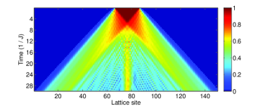
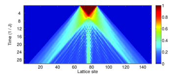
Figure 2: (color online) Time evolution of $\sqrt{n_{i\,\uparrow}(t)}$ (above) and $\sqrt{n_{i\,\uparrow\downarrow}(t)}$ (below) for $|U|=0.0$. The free-particle nature of the expansion is clear from the absence of separate doublon expansion wavefronts.

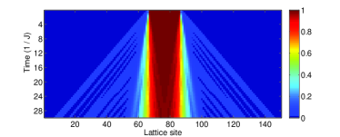
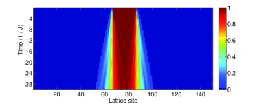
Figure 3: (color online) Same as Fig. 2 for $|U|=10.0$. For this interaction it is possible to distinguish the two wavefronts.

In the non-interacting case in Fig. 2, both particles and doublons are expanding at the speed of $2J$, corresponding to the highest group velocity allowed by the dispersion relation (see supplementary material). For strong interactions (Fig. 3), we see two separate wavefronts. Such separation into two types of wavefronts is clearly observable for interactions $|U|>3.0$. The outermost wavefront consists of fully unpaired particles expanding at the of speed $2J$, like in the $U=0$ case. In contrast doublons expand at the speed of $4J^{2}/U$ (see supplementary material for the explanation of these results).

Intermediate interactions $0.5\leq|U|\leq 3.0$ show a more complicated behaviour. The separate expansion fronts are no longer well distinguishable, suggesting a stronger interplay between single particles and doublons. Moving to even lower interactions, the unpaired particles and the doublons behave similarly to the case of $U=0$. Let us now examine the time dependence of the number of unpaired (up) particles $n_{i\,\uparrow}^{un}(t)$ for $|U|=5.0$ (Fig. 4).

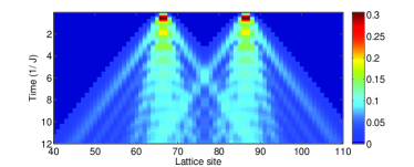
Figure 4: (color online) Unpaired particle expansion $n_{i\,\uparrow}^{un}(t)$ for $|U|=5.0$, exhibiting the oscillations described in the text.

Initially the dynamics in the band insulator cloud is Pauli blocked, since neighbouring lattice sites in the center have unit density for both spin up and down. Therefore the unpaired expansion fronts are created at the edges of the cloud. Intriguingly, $n_{i\,\uparrow}^{un}(t)$ shows damped oscillations at the edges associated with the emission of unpaired particles into the empty lattice. Considering the time evolution of $n_{E_{L},\uparrow}^{un}+n_{O_{L},\uparrow}^{un}$ (the two edge sites) over the whole interaction range $|U|=0.0-15.0$ (see Fig. 5 for $|U|=5.0,\,10$) we find that there are fewer periods of oscillations for lower interactions (for $|U|=1.0$ only one broad oscillation peak is visible) and the oscillation frequency increases with interaction strength, see supplementary material for a general survey of the data.

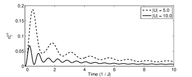
Figure 5: Unpaired population dynamics $n_{E_{L}+O_{L},\uparrow}^{un}(t)$ for $|U|=5.0$ and $|U|=10.0$.

The evolution of doublons into unpaired particles plays a key role in the expansion physics. For this reason, we focus now on the explanation of the oscillations in the case of high interactions, see Figs. 4 and 5. Our hypothesis is that one can consider the edges of the cloud (sites $E_{L}$, $O_{L}$ and $O_{R}$, $E_{R}$) at short timescales as two-site systems (Hubbard dimers Essler et al. (2005); Giamarchi (2003)). Focusing on the $E_{L}$/$O_{L}$ dimer, the system can be described as an initially empty state $|\emptyset\rangle$ in the left lattice site $E_{L}$ and a doublon $|\uparrow\downarrow\rangle$ in the right lattice site $O_{L}$. The dynamics of the dimer with this initial state can be solved analytically by diagonalizing its Hamiltonian (see supplementary material). As a result, in the two-site problem, the population of unpaired up particles on the two sites $E_{L}$ and $O_{L}$ is given by (the tilde refers to the Hubbard dimer model):

$$\tilde{n}_{E_{L}+O_{L},\uparrow}^{un}(t)=\frac{1-\cos(\sqrt{U^{2}+16J^{2}}t)}{2+\frac{U^{2}}{8J^{2}}}.$$ (1)

We extract the oscillation frequencies from the numerical Fourier transform (FT) of $n_{E_{L}+O_{L},\uparrow}^{un}$ and compare its peaks to the oscillation frequency $\sqrt{U^{2}+16J^{2}}$ in (1) (see Fig. 6). Moreover, we compare the height of the first peak of the unpaired density oscillations (seen in Figs. 4 and 5) to the amplitude $8/\left(16+\frac{U^{2}}{J^{2}}\right)$, in Fig. 7.

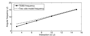
Figure 6: The frequency given by the FT of $n_{E_{L}+O_{L},\uparrow}^{un}(t)$ (from TEBD numerics) compared to the frequency $\sqrt{U^{2}+16J^{2}}$ obtained by solving the two-site model.

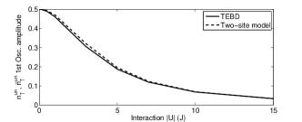
Figure 7: The height of the first peak of $n_{E_{L}+O_{L},\uparrow}^{un}(t)$ (from TEBD numerics) compared to the amplitude obtained by solving the two-site model.

The agreement is good considering that, for longer times, the FT of $n_{E_{L}+O_{L},\uparrow}^{un}(t)$ has additional contributions stemming from the hopping between the dimer and the rest of the chain. However, as the frequency is approximately $U$ in the high interaction limit, one might claim that the frequency correspondence could be obtained from simple energy arguments. Therefore, to further confirm the validity of the Hubbard Dimer model, we now move on to examine whether the two-site model coupled to the next adjacent sites explains the decay observed in $n_{E_{L}+O_{L},\uparrow}^{un}(t)$ (see Fig. 5). Let us define the damping $D$ to mean the decrease of the amplitude of the unpaired density oscillations, compared to $t=0$. We propose that the damping should be equal to the probability of having an unpaired particle in the Hubbard dimer times the probability for this single particle tunnelling out of this system. The probability for the single particle tunnelling (obtained by solving the two-site system with the initial state $|\emptyset,\uparrow\rangle$) is given by $\sin^{2}(J\,t)$. Combining this result with Eq.(1), we obtain the damping at a given time $\tau$:

$$D(\tau)=2\int_{0}^{\tau}\frac{1-\cos(\sqrt{U^{2}+16J^{2}}t)}{2+\frac{U^{2}}{8J^{2}}}\sin^{2}(J\,t)dt,$$ (2)

where the factor of two comes from the particle-hole symmetry: particles leaking out from the dimer to the left (to $E_{L}-1$) are mirrored by holes leaking to the right (to $O_{L}+1$) thus generating particle-like expansion fronts emitted out of the initial cloud and hole-like expansion fronts emitted into the cloud. When the particle-like and hole-like expansion fronts meet interference in the unpaired particle density is visible, see Fig. 4.

By comparing the decay predicted in Eq. (2) to the numerics, we observe that, for the duration of the first half-period, the decay is negligible. This is in accordance with the height of the first peak being equal to the two-site oscillation amplitude, as shown in Fig. 7. After three half-periods we compare the damping as predicted by Eq. (2) to the change of amplitude between the first peak and the second peak seen in numerics, see Fig. 8. The two-site model is again in good agreement with TEBD for $|U|>3.0$. The time beyond which Eq. (2) fails to describe the expansion physics is when the population of unpaired particles in the sites $O_{L+1},E_{L-1}$ becomes significant. This occurs when the $sin^{2}(Jt)=\frac{1-2cos(2Jt)}{2}$ term is no longer close to zero, limiting our short time analysis to times $t<<\frac{\pi}{2}\frac{1}{J}$. When U is sufficiently large, the Hubbard dimer oscillations occur in much shorter timescale than the single particle tunneling does. In other words, a large number of oscillations occur in the window $0<t<\frac{\pi}{2}\frac{1}{J}$ In the case of lower interactions, Hubbard Dimer oscillations at frequency $\sqrt{U^{2}+16J^{2}}$ become comparable to the frequency $2J$ and therefore we see that already the first oscillation peaks are heavily damped.

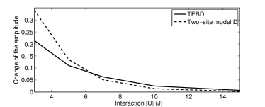
Figure 8: Change of the amplitude of $\tilde{n}_{E_{L},\uparrow}^{un}(t)$ oscillations after $t=\frac{3\pi}{\sqrt{U^{2}+16J^{2}}}$, compared to the change of amplitude between the first and second oscillation peaks of $n_{O_{L}+E_{L},\uparrow}^{un}(t)$ observed in TEBD numerics.

In general, the two-site dynamics is well able to describe the creation of the particle, hole, and doublon wavefronts seen in the density profiles. These wavefronts are created during the two-site oscillations. Our numerical results and analytical investigations confirm the two-fluid picture of the system. Initially, the interaction takes place at the edges of the cloud, where unpaired particles are created according to the dimer dynamics described above. The subsequent expansion is explained by dynamics of non-interacting particles (at the speed of $2J$) or doublons (at the speed of $4J^{2}/U$). Our model gives an excellent quantitative description in the highly-interacting limit due to the clear separation of the expansion and dimer oscillation eigenfrequencies. For interactions $0.5\leq|U|\leq 3.0$ the interplay between the expansion and the Hubbard dimer dynamics does not allow a quantitative description of the numerical results, however it provides a qualitative framework for further analysis. For $|U|\leq 0.5$, the free-particle expansion seems to give a fairly good description.

Finally, we compare our results to the 2D experiment of Schneider et al. (2010) done at finite temperature. We suggest that our two-site considerations also apply to the dynamics of the experiment. In 2D there is coupling to four adjacent sites, but just like in 1D, initially the sites are either Pauli blocked or empty. The simplified dynamics should originate from the two-site analysis, and subsequent short-time dynamics in the high interaction limit correspond to the two-fluid expansion, with the two fluids interacting only at the edges.

In order to compare our results to Fig. 5 of Schneider et al. (2010) we define the core density as $n_{i\,\uparrow}^{C}(t)=n_{i\,\uparrow}(t)-n_{i\,\uparrow}^{b}(t)$ for $|U|>0.5$ and $n_{i\,\uparrow}^{C}(t)=n_{i\,\uparrow}(t)$ for $|U|\leq 0.5$, where $n_{i\,\uparrow}^{b}(t)$ is the density of purely ballistic particles (see supplementary material). The definition of the core then corresponds to the diffusive part of the cloud in the model of Schneider et al. (2010). The core expansion velocity is given by $\dot{R}(t)$, where $R(t)=\sqrt{<i^{2}>-<i>^{2}}$, $<i>=\sum_{i=1}^{L}([n_{i\,\uparrow}^{C}(t)+n_{i\,\downarrow}^{C}(t)]*i)/\sum_{i=1}^{L}(n_{i\,\uparrow}^{C}(t)+n_{i\,\downarrow}^{C}(t))$ and $L$ is the number of lattice sites. The core expansion speed as a function of interaction is plotted in Fig. 9. The behavior of $\dot{R}(t)$ is indeed similar to the core expansion velocity in Fig. 5 of Schneider et al. (2010), showing also the negative velocities.

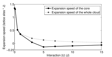
Figure 9: The core expansion speed $\dot{R}(t)$, as a function of the interaction strength. For reference, we plot also the expansion speed of the whole cloud.

Another recent experiment Sommer et al. (2010) studied collision dynamics of two Fermi gas clouds. Although the experiment is not done in a lattice, the theoretical framework presented here can in the low density limit be used to desribe also physics in Sommer et al. (2010), c.f. Kajala et al. (2011).

In conclusion, we studied the expansion of an interacting fermionic gas in a 1D lattice. We showed that the time evolution of this system can be described in terms of a two-fluid model of unpaired particles and doublons whose interplay gives rise to nontrivial dynamics. We suggest that the experimental results of Schneider et al. (2010) can be interpreted in terms of the analysis performed here. Our results should be widely applicable since expansion is a basic dynamics problem related to the ultracold gas experiments in particular, and to the transport properties of fermions in general.

I Expansion dynamics in the one-dimensional Fermi-Hubbard model - Supplementary material

II Survey of the numerical results

II.1 Density profiles

We show in Figs. 10 and 11 the time evolution of the (square-root) density for unpaired particles $\sqrt{n_{i\,\uparrow}(t)}$ and doublons $\sqrt{n_{i\,\uparrow\downarrow}(t)}$ for different values of the interaction. While the outermost wavefront velocity ($2J$), being related to the expansion of the unpaired particles, in Fig. 10 is interaction-independent, the doublon wavefronts in Fig. 11 have an interaction-dependent velocity ($4J^{2}/U$). In order to give grounds for our choice to plot the square root of unpaired particles and doublons in the article, in Figs. 12 and 13 we compare the square root densities and the densities for $|U|=10.0$. It is noted that we have studied the time evolution up to time t = 30 1/J. At this time the expanding cloud has not reached the edges of our finite system. However, the finite size causes low-momentum cutoff in the expansion dynamics. Therefore, we have experimented with systems of different size and we have seen that the lattice size does not affect the expansion dynamics significantly.

II.2 Doublon and unpaired particle oscillations

In the main article, we compare the oscillation of the unpaired population in the Hubbard dimer $\tilde{n}_{E_{L}+O_{L},\uparrow}^{un}(t)$ to its counterpart obtained with the TEBD algorithm $n_{E_{L}+O_{L},\uparrow}^{un}(t)$. In Fig. 14 the number of doublons in the whole lattice $n^{Total}_{i,\uparrow\downarrow}(t)$ as a function of time for various interactions are shown, exhibiting increasing oscillation frequency with increasing $|U|$. In Figs. 15 and 16 we show the Fourier transform (FT) of $n_{E_{L}+O_{L},\uparrow\downarrow}(t)$ and of $n^{Total}_{i,\uparrow\downarrow}(t)$ for $|U|=5$. Owing to particle-number conservation $n_{E_{L}+O_{L},\uparrow}^{un}(t)$ shows the same time oscillatory dependence as $n_{E_{L}+O_{L},\uparrow\downarrow}(t)$, although naturally in the opposite phase. The presence of extra peaks present in the FT of $n_{E_{L}+O_{L},\uparrow\downarrow}(t)$ with respect to the FT of $n_{E_{L}+O_{L},\uparrow}^{un}(t)$ will be explained later.

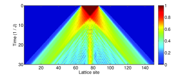
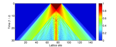
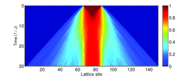
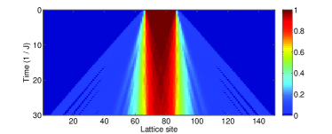
Figure 10: The square root of up density profiles $\sqrt{n_{i\,\uparrow}(t)}$. $|U|=0,0.1,1.0,5.0,10.0$ (top left to bottom right)

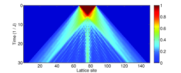
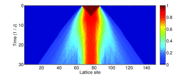
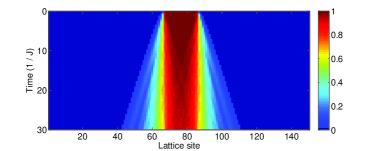
Figure 11: The square root of doublon density profiles. $|U|=0,0.1,1.0,5.0,10.0$ (left to right, top to bottom)

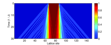
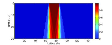
Figure 12: Comparison between the square root of the density profile $\sqrt{n_{i\,\uparrow}(t)}$ (left) with the density profile $n_{i\,\uparrow}(t)$(right) for $|U|=10.0$.The unpaired particle wavefronts expanding with speed $2J$ are clearly visible in the former.

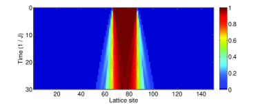
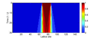
Figure 13: Comparison between the square root of the doublons density profile $\sqrt{n_{i\,\uparrow\downarrow}(t)}$ (left) with the density profile $n_{i\,\uparrow\downarrow}(t)$(right) for $|U|=10.0$. In the left panel ( $\sqrt{n_{i\,\uparrow\downarrow}(t)}$) low-density features are enhanced.

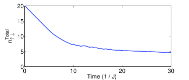
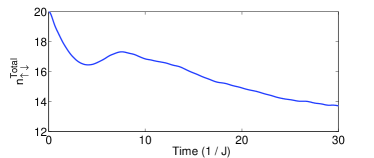
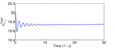
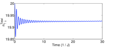
Figure 14: The time dependence of $n^{Total}_{i,\uparrow\downarrow}(t)$ for $|U|=0.1,1.0,5.0,10.0$ (top left to bottom right)

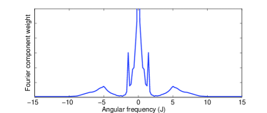
Figure 15: The Fourier transform of $n_{E_{L}+O_{L},\uparrow\downarrow}(t)$ for U=5.0.

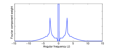
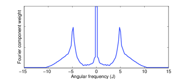
Figure 16: Fourier transform of $n^{Total}_{\uparrow\downarrow}(t)$ for U=3.0 (left) and U=5.0 (right)

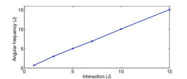
Figure 17: The position of the peaks in the Fourier transform of $n_{E_{L}\,\uparrow\downarrow}(t)$ as a function of the interaction strength.

In the numerics the FT $n_{E_{L}+O_{L},\uparrow\downarrow}^{un}(t)$ shows extra peaks with respect to the dimer dynamics which are associated to the hopping between the dimer and the rest of the chain. The peak at $\omega\simeq U$, present both for $n^{Total}_{\uparrow\downarrow}(t)$ and $n_{E_{L}+O_{L},\uparrow\downarrow}(t)$, correspond to the doublon dissociation frequency, as it will be later shown.

III The Hubbard dimer model

The eigenstates of the two-site Hubbard Hamiltonian (so called Hubbard dimer)

$$H=H_{J}+H_{int}$$

$$H_{J}=-J\sum_{\sigma}c^{\dagger}_{1,\sigma}c_{2\,\sigma}+h.c.$$

$$H_{int}=U\sum_{i=1,2}n_{i\,\uparrow}n_{i\,\downarrow}$$ (3)

are given by (see e.g. Trotzky et al. (2008))

$$|T\rangle=\frac{1}{\sqrt{2}}\left(|\uparrow,\downarrow\rangle+|\downarrow,\uparrow\rangle\right)$$

$$|D_{-}\rangle=\frac{1}{\sqrt{2}}\left(|\uparrow\downarrow,0\rangle-|0,\uparrow\downarrow\rangle\right)$$

$$|v_{\pm}\rangle=\frac{1}{\sqrt{1+\alpha_{\pm}^{2}}}\left(|S\rangle+\alpha_{\pm}|D_{+}\rangle\right),$$ (4)

where

$$\alpha_{\pm}=-\frac{U}{4J}\left[1\pm\sqrt{1+\frac{16J^{2}}{U^{2}}}\right],$$ (5)

$$|S\rangle=\frac{1}{\sqrt{2}}\left(|\uparrow,\downarrow\rangle-|\downarrow,\uparrow\rangle\right)$$ (6)

$$|D_{+}\rangle=\frac{1}{\sqrt{2}}\left(|\uparrow\downarrow,0\rangle+|0,\uparrow\downarrow\rangle\right)$$ (7)

and the corresponding eigenvalues have the following form

$$\begin{array}[]{ll}\lambda_{-}=U/2\left[1-\sqrt{1+\frac{16J^{2}}{U^{2}}}\right](<0)&\Leftrightarrow\qquad|v_{-}\rangle\\ \lambda_{0}=0&\Leftrightarrow\qquad|T\rangle\\ \lambda_{U}=U&\Leftrightarrow\qquad|D_{-}\rangle\\ \lambda_{+}=U/2\left[1+\sqrt{1+\frac{16J^{2}}{U^{2}}}\right](>U)&\Leftrightarrow\qquad|v_{+}\rangle.\end{array}$$ (8)

III.1 Hubbard dimer dynamics

We can apply the approach described in the previous section to the analysis of the edge sites of the cloud. As described in the main article, the edges of the cloud can be described as Hubbard dimers. If we focus on the system $E_{L}+O_{L}$, the initial state is given by

$$|\phi(t=0)\rangle=|0,\uparrow\downarrow\rangle=\frac{1}{\sqrt{2}}(\gamma_{+}|v_{+}\rangle-\gamma_{-}|v_{-}\rangle-|D_{-}\rangle)$$ (9)

where we have denoted

$$\gamma_{\pm}=\frac{1}{(\alpha_{+}-\alpha_{-})}\frac{1}{\sqrt{1+\alpha_{\pm}^{2}}}.$$ (10)

The number of doublons in the initially empty site $E_{L}$ is given by

$$n_{E_{L}+O_{L},\uparrow\downarrow}(t)= \langle 0,\uparrow\downarrow|e^{\frac{i\hat{H}t}{\hbar}}\,\hat{n}^{L}_{\uparrow\downarrow}\,e^{-\frac{i\hat{H}t}{\hbar}}|0,\uparrow\downarrow\rangle$$

$$= \frac{1}{4}+\frac{\alpha^{2}_{+}+\alpha^{2}_{-}}{4(\alpha_{+}-\alpha_{-})^{2}}+\frac{1}{2(\alpha_{+}-\alpha_{-})^{2}}$$ (11)

$$-\left[\frac{\alpha_{+}\alpha_{-}+1}{2(\alpha_{+}-\alpha_{-})^{2}}\right]\cos\left[(\lambda_{+}-\lambda_{-})t\right]$$

$$-\frac{\alpha_{+}}{2\left(\alpha_{+}-\alpha_{-}\right)}\cos\left[(\lambda_{U}-\lambda_{+})t\right]$$

$$+\frac{\alpha_{-}}{2\left(\alpha_{+}-\alpha_{-}\right)}\cos\left[(\lambda_{U}-\lambda_{-})t\right].$$

Straightforwardly, Eq. (III.1) allows to evaluate the number of unpaired particles in the same site

$$n_{E_{L}+O_{L},\uparrow}(t)= \frac{1}{4}+\frac{\alpha^{2}_{+}+\alpha^{2}_{-}}{4(\alpha_{+}-\alpha_{-})^{2}}+\frac{1}{2(\alpha_{+}-\alpha_{-})^{2}}$$ (12)

$$-\left[\frac{\alpha_{+}\alpha_{-}}{2(\alpha_{+}-\alpha_{-})^{2}}+\frac{1}{2(\alpha_{+}-\alpha_{-})^{2}}\right]$$

$$*cos\left[(\lambda_{+}-\lambda_{-})t\right]$$

$$-\frac{\alpha_{+}}{2\left(\alpha_{+}-\alpha_{-}\right)}\cos\left[(\lambda_{U}-\lambda_{+})t\right]$$

$$+\frac{\alpha_{-}}{2\left(\alpha_{+}-\alpha_{-}\right)}\cos\left[(\lambda_{U}-\lambda_{-})t\right].$$

The extra peaks appearing in the FT of $n_{E_{L}+O_{L},\uparrow\downarrow}(t)$ (Fig. 15), with respect to the FT of $n^{Total}_{\uparrow\downarrow}(t)$ (Fig. 16 are due to the fact that, on top of the doublon dissociation dynamics, $n_{E_{L}+O_{L},\uparrow\downarrow}(t)$ is affected by the hopping of both unpaired particles and doublons in and out of the dimer $E_{L}/O_{L}$. These contributions, since a sum over the whole cloud is carried out, add up to zero for $n^{Total}_{\uparrow\downarrow}(t)$.

IV Expansion velocities for particles and doublons

The expansion velocity of the unpaired particles can be easily obtained considering the dispersion relation of a particle hopping through on an empty lattice

$$\epsilon_{k}=-2J\cos(k)$$ (13)

leading to the group velocity

$$v_{k}=\frac{\partial\epsilon_{k}}{\partial k}=2J\sin(k).$$ (14)

Since in our system we consider particles generated at a specific site ($E_{L}$), all momentum states contribute to the expression of the initial state. From Eq. (14) we thus see that the maximum velocity is attained for $k=\pi/2$

$$v^{un}_{max}=2J\sin(k)\big{|}_{k=\frac{\pi}{2}}=2J$$ (15)

which corresponds to the value obtained in the TEBD simulation. Analogously it can be shown that, for our initial configuration, the doublon hopping corresponds to the hopping of a particle with $J_{eff}=\frac{4J^{2}}{U}$ Giamarchi (2003); Essler et al. (2005); Winkler et al. (2006) corresponding to the velocity of propagation of a charge excitation in the strongly attractive Hubbard model. In particular, if we consider the case where no unpaired particles are present, we can map our system to an isotropic Heisenberg chain by identifying $|\uparrow\downarrow\rangle\Rightarrow|\uparrow\rangle$ and $|\emptyset\rangle\Rightarrow|\downarrow\rangle$. To prove this, we consider:

1. A staggered particle-hole transformation

   $$c^{(\dagger)}_{i\,\uparrow}\Rightarrow c^{(\dagger)}_{i\,\uparrow}$$ (16)

   $$c^{\dagger}_{i\,\downarrow}\Rightarrow(-1)^{i}c_{i\,\downarrow}$$ (17)

   $$c_{i\,\downarrow}\Rightarrow(-1)^{i}c^{\dagger}_{i\,\downarrow}$$ (18)

   which transforms our original system (filling $n=\sum_{i\,\sigma}n_{i\,\sigma}/L$, magnetization density $m=0$ and interaction strength $U$) to a half-filled system with filling $n^{\prime}=1$, magnetization density $m^{\prime}=n-1$ and interaction strength $U^{\prime}=-U$. Since $n^{\prime}_{i\,\uparrow}=n_{i\,\uparrow\downarrow}\\ n^{\prime}_{i\,\downarrow}=1-n_{i\,\uparrow\downarrow}$;

2. by strong coupling second order expansion Essler et al. (2005), the system Hamiltonian is then mapped to an isotropic Heisenberg Hamiltonian

   $$H_{H}=-\frac{4J^{2}}{U}\sum_{i}\overrightarrow{S}_{i}\overrightarrow{S}_{i+1}.$$ (20)

   With the mappings described above, since a doubly occupied site correspond to a spin up, and an empty site to a spin down, the band-insulator initial state $\left|\phi(0)\right\rangle$ is thus transformed to a spin chain with $O_{R}-O_{L}$ central spin-up sites surrounded by spin-down sites, and the expansion dynamics of the doublons corresponds to the propagation of a single spin-up excitation through a spin-down polarized system. Its dispersion relation is given by

   $$\epsilon_{k}^{spin}=\frac{4J^{2}}{U}\cos(k)$$ (21)

   and hence, analogously to the derivation of the maximum velocity for the unpaired particles, to

   $$v_{MAX}^{doublon}=v_{MAX}^{spin}=\left|\frac{4J^{2}}{U}\right|.$$ (22)

V Definition of the core

We have in the high interaction limit ballistic particles emitted from the diffusive core, the two types of ballistic particles being unpaired particles and doublons. These two expand at constant speeds ($2J$ and $\frac{4J^{2}}{U^{2}}$) in wavefronts whose densities are so low that spin-spin scattering (i.e. the Hubbard Dimer dynamics) is negligible. In contrast, the core has high density, the Dimer dynamics occur, and thus the core is diffusive. In the case of interactions lower than $|U|<3$ also the densities of the unpaired and doublon wavefronts become high enough for the Dimer Dynamics, which in the language of the classical non-linear diffusion model in Schneider et al. (2010) makes the two types of wavefronts diffusive. This diffusive behaviour is seen in our results as the absence of ballistic wavefronts in density profiles (see e.g. the $|U|=1.0$ case in Fig. 10 above). Finally, for the very low interactions $U\leq 0.5$ the problem simplifies to ballistic expansion of non-interacting particles.

In order to compare our results to Fig. 5 of Schneider et al. (2010) we arrive at the problem of defining the core. In the high interaction limit this is perhaps easier as the ballistic particles clearly separate from the central diffusive region, the core. In the middle interaction region (see again the $U=1.0$ case in Figs. 10 and 11 below ) we see that only one outermost wavefront expands ballistically and therefore if we consider the diffusive region of the cloud to be the core then the core would be everything else but the outermost wavefront. This definition however is problematic in the low interaction limit (U $\leq$ 0.5). In this limit everything can be described as expansion of non-interacting ballistic particles. So the definition of the core as the diffusive part of the cloud does not work any more as then we would not have a core at all.

However, experimentally it might be easier to define a high density region to correspond to the core, and fit the half-power half-maximum of a Gaussian to give the core width and subsequently the core expansion speed. In effect, then, in the low interaction regime the core is defined as the whole cloud, and in the middle and high interaction regimes the core is defined as everything else except the ballistic expansion fronts. This is what we have done in the main article.

A variation of the above way of removing ballistic contributions would be to remove only the ballistic particle wavefronts, as the ballistic hole wavefronts may in effect be included in the experimental high density core region. To elaborate on what the hole wavefronts are, in the core state $|\uparrow\downarrow\rangle$ changes into a superposition of $|\uparrow>$ and $|\downarrow\rangle$. This decreases the total density, but in addition the $|\uparrow\rangle$ and $|\downarrow\rangle$ states created are now part of a singlet state which expands ballistically into the core. So, if we want to define the core to be everything that is not ballistic, we need also to remove the density contribution of the ballistic singlets in the core. Thus there are two reasonable approaches in defining the core. First is that we remove everything that is ballistic (particles and holes) and the second is that we remove only the particles. The core expansion speeds obtained in these two ways are plotted in 18. Both methods result in negative core expansion velocities as seen in the experiment Schneider et al. (2010).

Figure 18: The core expansion velocities obtained by removing ballistic contributions (see text).

VI The time evolution of charge-charge correlations

Using TEBD we can calculate correlation functions during the expansion of the cloud. An interesting correlation function in the case of the band insulator expansion is the charge-charge correlator $C_{ij}(t)$, given by

$$C_{i,j}(t)=<\Phi(t)|(\hat{n}_{i,\uparrow}+\hat{n}_{i,\downarrow})(\hat{n}_{j,\uparrow}+\hat{n}_{j,\downarrow})|\Phi(t)>.$$ (23)

However, $C_{ij}(t)$ is dominated by single particle density correlations. To see the effect of the non-trivial correlations, we want to remove the density-density correlations from $C_{i,j}(t)$. If $i\neq j$ the density-density correlations are given by $<\hat{n}_{i,\uparrow}><\hat{n}_{ji,\uparrow}>+<\hat{n}_{i,\downarrow}><\hat{n}_{j,\downarrow}>+<\hat{n}_{i,\uparrow}><\hat{n}_{j,\downarrow}>+<\hat{n}_{i,\downarrow}><\hat{n}_{j,\uparrow}>$. When $i=j$, $<n_{i,\uparrow}n_{i,\uparrow}>=<c^{\dagger}_{i,\uparrow}c_{i,\uparrow}c^{\dagger}_{i,\uparrow}c_{i,\uparrow}>=<c^{\dagger}_{i,\uparrow}(1-c^{\dagger}_{i,\uparrow}c_{i,\uparrow})c_{i,\uparrow}>=<c^{\dagger}_{i,\uparrow}c_{i,\uparrow}>=n_{i,\uparrow}$ and therefore on the diagonal the we just remove the single particle and doublon densities. Therefore, the correlation function which displays the non-trivial correlations is

$$D_{i,j}(t)=C_{i,j}(t)-(<\hat{n}_{i,\uparrow}><\hat{n}_{j,\uparrow}>$$

$$+<\hat{n}_{i,\downarrow}><\hat{n}_{j,\downarrow}>$$

$$+<\hat{n}_{i,\uparrow}><\hat{n}_{j,\downarrow}>$$

$$+<\hat{n}_{i,\downarrow}><\hat{n}_{j,\uparrow}>)$$

$$(1-\delta_{ij})$$

$$-(<\hat{n}_{i,\uparrow}>+<\hat{n}_{i,\downarrow}>$$

$$+2<\hat{n}_{i,\uparrow\downarrow}>)\delta_{ij}.$$ (24)

The square root of the correlator $D_{i,j}(t)$ is plotted in Figs. 19 and 20 for $|U|=5.0$ at times $4\frac{1}{J},8\frac{1}{J},12\frac{1}{J},16\frac{1}{J}$. At time $t=0\frac{1}{J}$ the correlator is zero everywhere. We plot the square root instead of the actual value to see better the low value regions of the correlator. While keeping $\Gamma=150$ during the time evolution in order to minimize the truncation error propagation, for the calculation of the correlators we have truncated the Schmidt number to $\Gamma=80$ due to heavy numerical cost of the calculation, since for the evaluation of an observable at a given time the introduced error is negligible. Our dimer picture is supported by the fact that most of the correlations arise between sites around the edges of the cloud. In addition to this, correlations arise between the wavefronts expanding in the initially free sites $i<E_{L}$ and $i>E_{R}$ and the whole initial cloud, corresponding to the stripes appearing in Figs. 19 and 20. A similar description can be applied to the holes propagating towards the center of the cloud. This behavior reflects the intrinsically collective nature of the excitations in 1D systems. Our picture of a ballistic particle leaving the cloud and a hole propagating towards the centre is complemented by this observation, which leads to the buildup of correlations between the propagating particles and the entire cloud.

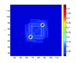
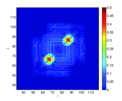
Figure 19: (color online) Left: $\sqrt{D_{i,j}(t)}$ for $|U|=5.0$ at $t=4\frac{1}{J}$. Right: The same for $t=8\frac{1}{J}$.

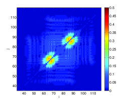
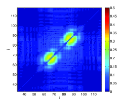
Figure 20: (color online) Left: The same as figure 19 but for $t=12\frac{1}{J}$ (left) and $t=16\frac{1}{J}$ (right).

VII References

References

- Trotzky et al. (2008) S. Trotzky, P. Cheinet, S. Folling, M. Feld, U. Schnorrberger, A. M. Rey, A. Polkovnikov, E. A. Demler, M. D. Lukin, and I. Bloch, Science 319, 295 (2008).
- Giamarchi (2003) T. Giamarchi, Quantum Physics in One Dimension (Oxford University Press, 2003).
- Essler et al. (2005) F. H. L. Essler, H. Frahm, F. Göhmann, A. Klümper, and V. E. Korepin, The One-Dimensional Hubbard Model (Cambridge University Press, 2005).
- Winkler et al. (2006) K. Winkler, G. Thalhammer, F. Lang, R. Grimm, J. Denschlag, A. Daley, A. Kantian, H. Büchler, and P. Zoller, Nature 441, 853 (2006).
- Schneider et al. (2010) U. Schneider, L. Hackermüller, J. P. Ronzheimer, S. Will, S. Braun, T. Best, I. Bloch, E. Demler, S. Mandt, D. Rasch, and A. Rosch, arXiv:1005.3545.