A Design and Implementation of the
Extended Andorra Model

Abstract

Logic programming provides a high-level view of programming, giving implementers a vast latitude into what techniques to explore to achieve the best performance for logic programs. Towards obtaining maximum performance, one of the holy grails of logic programming has been to design computational models that could be executed efficiently and that would allow both for a reduction of the search space and for exploiting all the available parallelism in the application. These goals have motivated the design of the Extended Andorra Model, a model where goals that do not constrain non-deterministic goals can execute first.

In this work we present and evaluate the Basic design for Extended Andorra Model (BEAM), a system that builds upon David H. D. Warren’s original EAM with Implicit Control. We provide a complete description and implementation of the BEAM System as a set of rewrite and control rules. We present the major data structures and execution algorithms that are required for efficient execution, and evaluate system performance.

A detailed performance study of our system is included. Our results show that the system achieves acceptable base performance, and that a number of applications benefit from the advanced search inherent to the EAM.

1 Introduction

Logic programming [Lloyd (1987)] (LP) relies on the idea that computation is controlled inference. LP provides a high-level view of programming where programs are fundamentally seen as a collection of statements that define a model of the intended problem. Queries may be asked against this model, and answers will be given through a proof procedure, such as refutation. Prolog [Colmerauer (1993)] is the most popular logic programming language. Prolog relies on SLD resolution [Hill (1974)], and uses a straightforward left-to-right selection function and depth-first search rule. This computation rule is simple to understand and efficient to implement but, unfortunately, it is not the ideal rule for every logic program. It is well known that for many programs the left-to-right selection function is not effective at constraining the search space and in the worst cases can lead to looping. Often, these limitations lead Prolog programmers to convoluted and non-declarative programs.

Ideally, one would like novel computational models for LP to achieve the following two goals, in order of priority [Warren (1990)]:

• Minimum number of inferences: by trying never to repeat the same execution step (inference) in different locations of the execution tree.

• Maximum parallelism: by allowing goals to execute as independently as possible, and combining all solutions as late as feasible.

Both goals can be achieved through a variety of techniques. Coroutining and tabling are nowadays widely used to reduce the number of inferences performed by logic programs [I.S.Laboratory (2004), Santos Costa et al. (2000), Aggoun et al. (1995), Sagonas et al. (1997)]. Coroutining allows goal execution when all required arguments are bound. Tabling avoids repeated computations of the same goal, and can be used to prevent infinite loops. Several forms of parallelism, such as and-parallelism between goals, and or-parallelism between alternatives, have been exploited in LP, with excellent results [Gupta et al. (2001)].

One should observe that the two goals of minimal inferences and of maximal parallelism are not independent. Indeed, work on concurrent LP languages showed the strong interplay between coroutining and and-parallelism [Ueda and Morita (1990), Ueda (2002)]. In the Basic Andorra Model (BAM) [Warren (1988)] coroutining between determinate goals (goals with at most one valid alternative) constrains the search space and generates and-parallelism, whereas the alternatives of non-deterministic goals generate or-parallelism. The Andorra-I prototype [Santos Costa et al. (1991a)] demonstrated the approach to be practical and effective. On the other hand, Andorra-I does depend on finding determinacy. If determinacy cannot be found efficiently, there is no benefit in using this model.

The Extended Andorra Model [Warren (1989)] (EAM) lifts the main restrictions in the BAM. The key ideas for this model can be described as:

• Goals can execute immediately (in parallel) as long as they are deterministic or they do not need to bind external variables;

• If a goal must bind external variables non-deterministically, the computation of this goal will split.

The EAM provides a generic model for the exploitation of coroutining and parallelism in LP, and motivated two main lines of research.

One approach was followed by Haridi, Janson and researchers at SICS who concentrated on the AKL [Janson and Haridi (1991)], the Agents Kernel Language, based on the principle that the advantages of the EAM justified a new programming paradigm that could subsume both traditional Prolog and the concurrent logic languages. AKL programs are formed of guarded clauses, where the guard is separated from the body through the sequential conjunction operator, cut, or commit. AKL systems obtained acceptable performance, both in sequential and parallel implementations, such as Penny [Montelius and Ali (1995), Montelius and Magnusson (1997)], but the language was not actively supported. Instead, the AKL researchers shifted their interest to Oz [Smolka (1995)]. This language provides some of the advantages of LP such as the logical variables, and of AKL such as encapsulation, but makes thread programming and search control fully explicit.

In contrast, David H. D. Warren and researchers at Bristol concentrated on the Extended Andorra Model with Implicit Control [Warren (1990)], where the goal was to apply the EAM as a technique to achieve efficient execution of logic programs, with minimal programmer effort. Gupta’s proof-of-concept interpreter [Gupta and Warren (1991)] showed the need for further research on the EAM, and presented new concepts such as lazy copying and eager producers that give finer control over search and improve parallelism. Gupta and Pontelli later experimented with an extension of dependent and-parallelism that provide some of the functionality of the EAM through parallelism, EDDAP [Gupta and Pontelli (1997)]. EDDAP shows how the EAM ideas are important in parallel logic programming systems.

In this work we present the BEAM, an implementation of the Extended Andorra Model for Logic Programs. Our research was motivated by the original question of whether the EAM can be an effective mechanism for the execution of logic programs, and this work extends the original EAM work by:

• Providing a complete description of an EAM kernel as a set of rewrite and control rules, and evaluating these rules through a prototype implementation [Lopes et al. (2003b)]. We call this kernel design the BEAM, Basic design for Extended Andorra Model [Lopes et al. (2001)]. Sections 2 and 3 present this contribution.

• Studying how to take the best advantage of the EAM with the least programmer intervention [Lopes et al. (2004)]. In the spirit of Kowalski’s original definition, and building upon Warren and Gupta’s original work [Gupta and Warren (1991)], we experimented with different approaches to exploiting control and contrast them to the guard-style approach used in AKL. Section 4 presents this contribution.

• Exploring novel implementation techniques for the EAM, including efficient support for deterministic computations [Lopes et al. (2003a)] and efficient memory management [Lopes and Santos Costa (2005)]. Sections 5 and 6 presents this contribution.

Our results show that the system achieves acceptable base performance, and that a number of applications benefit from the advanced search inherent to the EAM. Moreover, we show that implicit control can be in fact quite effective for a sizeable number of applications, and that simple annotations can contribute to further improvements with little programmer effort.

This paper is organised as follows. Section 2 presents the main BEAM concepts, that fully specify an Extended Andorra Model with implicit control. Next, in Section 3 we propose a number of rules that simplify and optimize the BEAM computational state. Section 5 shows the BEAM implementation. Section 6 discusses memory management issues, and Section 7 focuses on emulator design. We evaluate the performance of our system in Section 8, and finish with Conclusions and a Discussion of Related Work. The reader is expected to have understanding of the key issues in Logic Programming implementation, and in particular of the design of the Warren Abstract Machine (WAM) [Warren (1983)].

2 BEAM Concepts

A BEAM computation is a sequence of rewriting operations performed on And-Or Trees. And-Or Trees are trees of and-boxes and or-boxes:

• An and-box $\Delta$ represents a conjunction:

  • $\displaystyle\hskip 25.00003pt{[\exists X_{1},\ldots,X_{m}:\sigma\makebox[0.6458pt]{}\&\makebox[0.6458pt]{}A_{1}\makebox[0.6458pt]{}\&\makebox[0.6458pt]{}\ldots\&\makebox[0.6458pt]{}A_{n}\makebox[0.6458pt]{}]\makebox[0.6458pt]{}\makebox[0.6458pt]{}(n\geq 0)}$

  Each $A_{i}$ in the conjunction may be a literal $G_{i}$ or an or-box. Initially, an and-box represents the body of a Horn clause and all $A_{i}$ are literals of the form $G_{i}$.

  A variable is said to be local to an and-box $\Delta$ when it is scoped at $\Delta$. The variables $X_{1}$ to $X_{m}$ represent the set of variables local to the box $\Delta$. Initially, these variables are the variables occurring in and only in the body of the clause $G_{1}\makebox[0.6458pt]{}\&\makebox[0.6458pt]{}\ldots\makebox[0.6458pt]{}\&\makebox[0.6458pt]{}G_{n}$.

  The set $\sigma$ is a set of constraints. In this work, we shall focus only on Herbrand constraints, and we may refer to them as bindings.

  The environment of an and-box consists of all variables local to the and-box and to every ancestor and-box. Variables local to an ancestor box are called external to the current and-box.

• An or-box $\Omega$ represents the matching clauses for a goal; each or-box contains a sequence of and-boxes $\Delta_{1}$ to $\Delta_{n}$.

  • $\displaystyle\hskip 25.00003pt{\{\Delta_{1}\vee\ldots\vee\Delta_{n}\}\makebox[0.6458pt]{}\makebox[0.6458pt]{}(n\geq 0)}$

  Each child and-box $\Delta_{i}$ initially represents an alternative clause for a goal.

A configuration is an And-Or Tree describing a state of the computation. Given a literal $Q$, the query, a computation is a sequence of configurations starting at the initial configuration, and obtained by successive applications of the rewrite rules defined next. The initial configuration is a single and-box such that:

• $X_{1},\ldots,X_{n}\mathchar 61\relax vars(Q)$

• $\sigma\mathchar 61\relax\emptyset$

• the literal $Q$.

The constraints over the uppermost and-box(es) on the final configuration are called the answer(s).

A goal, or literal, is said to be deterministic when the corresponding or-box has at most one and-box. Otherwise it is said to be non-deterministic.

An and-box $\Delta$ is said to be suspended if only the splitting rule, defined in section 2.1, applies to $\Delta$ and if there is at least one variable $X$ such that binding $X$ will allow applying a different rule to $\Delta$.

2.1 Rewrite Rules

Execution in the EAM proceeds as a sequence of rewrite operations on configurations. The BEAM’s rewrite rules are based on David H. D. Warren’s proposal [Warren (1990)]. They have been designed to allow for efficient implementation. In the following we use square brackets to represent an and-box $\Delta$, curly brackets to represent an or-box $\Omega$, and the symbol $G$ to refer an unfolded literal (sub-goal), and the symbols $A$ and $B$ to refer a sequence with literals and or-boxes. We present the rewrite rules both graphically and textually. Graphically, the leftmost box is the original configuration and the rightmost box the transformed configuration. Textually, the configuration above the line is transformed into the configuration below the line.

The BEAM rewrite rules are as follows:

Reduction

This rule resolves a goal $G$ in an and-box against the heads of all clauses defining the procedure for $G$. The rule always creates a new or-box and one and-box for each clause that unifies with the goal. Each and-box $i$ is initialised with the most general unifier between the clause’s head and the goal, $\sigma_{i}$, and with the set of existential variables in the clause, ${\mathcal{}Y}_{i}$. $A$ and $B$ denote conjunctions of goals.

• $\displaystyle\hskip 25.00003pt{\begin{array}[]{lc}&[\exists{\mathcal{}X}:\sigma\&A\&G\&B]\\ (Reduction)&\longrightarrow\\ &{[}\exists{\mathcal{}X}:\sigma\&A\&\left\{\begin{array}[]{c}{[}\exists{\mathcal{}Y}_{1}:\sigma_{1}\makebox[0.6458pt]{}\&\makebox[0.6458pt]{}G_{11}\&\ldots\&\makebox[0.6458pt]{}G_{1k}]\\ \lor\ldots\lor\\ {[}\exists{\mathcal{}Y}_{n}:\sigma_{n}\makebox[0.6458pt]{}\&\makebox[0.6458pt]{}G_{n1}\&\ldots\&\makebox[0.6458pt]{}G_{nk}]\end{array}\right\}\&B]\end{array}}$

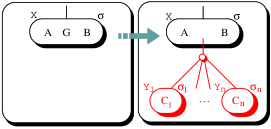
Figure 1: BEAM reduction rule. Each $C_{i}$ represents the body of a clause $G_{i1}\makebox[0.6458pt]{}\&\ldots\&\makebox[0.6458pt]{}G_{ik}$

Figure 1 shows how resolution expands the tree. Notice that the new variables created by the rewrite rule are guaranteed to be standardised apart. Also, the reduction rule just unfolds goal $G$, no constraint propagation is performed from below to above, even if the or-box has a single child.

Promotion

This rule promotes the variables and constraints from an and-box $\Delta$ to the closest ancestor and-box $\Delta^{\prime}$:

• $\displaystyle\hskip 25.00003pt{\begin{array}[]{lc}&[\exists{\mathcal{}X}:\sigma\makebox[0.6458pt]{}\&\makebox[0.6458pt]{}A\makebox[0.6458pt]{}\&\makebox[0.6458pt]{}\{[\exists{\mathcal{}Y}:\theta\makebox[0.6458pt]{}\&\makebox[0.6458pt]{}W]\}\makebox[0.6458pt]{}\&\makebox[0.6458pt]{}B]\}\\ (Promotion)&\longrightarrow\\ &{[}\exists{\mathcal{}X},{\mathcal{}Y}:\sigma\theta\makebox[0.6458pt]{}\&\makebox[0.6458pt]{}A\makebox[0.6458pt]{}\&\makebox[0.6458pt]{}\{[W]\}\makebox[0.6458pt]{}\&\makebox[0.6458pt]{}B]\end{array}}$

The BEAM allows promotion only if $\Delta$ is the single alternative to the parent or-box, as illustrated in Figure 2. The box $\Delta$ is represented by the round box that contains goal W and $\Delta^{\prime}$ is represented by the round box that contains A and B. $\sigma\theta$ is the composition of constraints $\sigma$ and $\theta$.

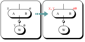
Figure 2: BEAM promotion rule.

Promotion follows Warren’s EAM rule in that it propagates results from a local computation to the level above. However, promotion in the BEAM does not simplify the structure of the tree, in contrast with the original EAM and with AGENTS [Janson and Montelius (1992)].

Propagation

This rule allows us to propagate a constraint $\sigma_{i}$ from an and-box to another and-box in the subtree below. This rule is thus symmetrical to the promotion rule.

• $\displaystyle\hskip 25.00003pt{\begin{array}[]{lc}&{[}\exists{\mathcal{}X},{\mathcal{}Z}:\sigma\&A\makebox[0.6458pt]{}\&\makebox[0.6458pt]{}\{\ldots\vee[\exists{\mathcal{}Y}:\theta\&W]\vee\ldots\}\makebox[0.6458pt]{}\&B]\makebox[0.6458pt]{}\makebox[0.6458pt]{}\land\makebox[0.6458pt]{}\makebox[0.6458pt]{}\sigma_{i}\in\sigma\\ (Propagation)&\longrightarrow\\ &{[}\exists{\mathcal{}X},{\mathcal{}Z}:\sigma\&A\makebox[0.6458pt]{}\&\makebox[0.6458pt]{}\{\ldots\vee[\exists{\mathcal{}Y}:\theta\sigma_{i}\&W]\vee\ldots\}\makebox[0.6458pt]{}\&B]\end{array}}$

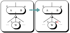
Figure 3: BEAM propagation rule.

Figure 3 shows how the propagation rule makes the constraint $\sigma$ available to the underlying and-boxes. Together, the promotion and propagation rules allow us to propagate bindings through the and-or tree.

Splitting

This rule is also known as non-determinate promotion. The rule distributes a cut-free conjunction across a disjunction, in a way similar to the original EAM’s forking rule [Warren (1989)].

• $\displaystyle\hskip 25.00003pt{\begin{array}[]{lc}&[\exists{\mathcal{}X}:\sigma\makebox[0.6458pt]{}\&\makebox[0.6458pt]{}A\makebox[0.6458pt]{}\&\{\Delta_{1}\lor\ldots\lor\Delta_{i}\lor\ldots\lor\Delta_{n}\}\makebox[0.6458pt]{}\&\makebox[0.6458pt]{}B]\\ (Splitting)&\longrightarrow\\ &\{[\exists{\mathcal{}X}:\sigma\makebox[0.6458pt]{}\&\makebox[0.6458pt]{}A\makebox[0.6458pt]{}\&\makebox[0.6458pt]{}\{\Delta_{i}\}\makebox[0.6458pt]{}\&\makebox[0.6458pt]{}B]\makebox[0.6458pt]{}\lor\\ &{[}\exists{\mathcal{}X}:\sigma\makebox[0.6458pt]{}\&\makebox[0.6458pt]{}A\makebox[0.6458pt]{}\&\makebox[0.6458pt]{}\{\Delta_{1}\lor\ldots\lor\Delta_{i\mathchar 45\relax 1}\lor\Delta_{i\mathchar 43\relax 1}\lor\ldots\lor\Delta_{n}\}\makebox[0.6458pt]{}\&\makebox[0.6458pt]{}B]\}\end{array}}$

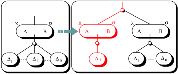
Figure 4: BEAM splitting rule.

As stated above, the parent and-box may not include a pruning operator as its direct element.

In contrast to the previous rules, splitting duplicates goals in the tree. It is therefore the most expensive rule in the BEAM, and as discussed next, the control strategy in the BEAM tries to delay application of splitting as much as possible.

3 Simplification Rules

We have presented the main rules that allow us to create and expand the tree, and to propagate bindings. An actual implementation must be able to simplify the And-Or Tree in order to propagate success and failure and in order to recover space by discarding boxes. The BEAM therefore includes additional simplification rules that generate compact configurations and allow us to optimize the computation process. These are:

Success-Propagation:

The original EAM does not explicitly provide a notion of successful computation, meaning a computation that has completed execution and that may now be discarded. The following rules identify success situations in the BEAM and allow the propagation of success towards the upper boxes. To implement these rules we use the notion of a true-box: an and-box is called a true-box when all the local computations have been completed and the and-box does not impose constraints on external variables:

• $\displaystyle\hskip 25.00003pt{[\exists{\mathcal{}X}:\emptyset]\equiv\mathtt{true}}$

Note that the and-box might initially have had constraints on external variables, but those constraints have left the and-box after application of the promotion rule. We say that a success occurs when we find a true-box.

• $\displaystyle\hskip 25.00003pt{\begin{array}[]{lc}(Success\mathchar 45\relax Propagation)&[\exists{\mathcal{}X}:\sigma\makebox[0.6458pt]{}\&\makebox[0.6458pt]{}A\makebox[0.6458pt]{}\&\makebox[0.6458pt]{}\{\mathtt{true}\}\makebox[0.6458pt]{}\&\makebox[0.6458pt]{}B]\longrightarrow[\exists{\mathcal{}X}:\sigma\makebox[0.6458pt]{}\&\makebox[0.6458pt]{}A\makebox[0.6458pt]{}\&\makebox[0.6458pt]{}B]\end{array}}$

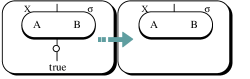
Figure 5: BEAM Success-Propagation rule.

If an or-box contains a unique alternative which succeeds, the or-box has succeeded and can be discarded (see Figure 5). True-boxes may also be used to achieve implicit pruning, as discussed below in section 3.1.

The ultimate goal of a BEAM computation is to reduce all and-boxes to true-boxes so that the initial and-box can itself be simplified.

Leftmost-Failure Propagation

The operation symmetric to the propagation of success is the propagation of failure. It is quite important to identify failed computations in order to allow the propagation of failure towards the upper boxes and in order to recover space. Again, the basic EAM design does not contain explicit rules for failure propagation. First, we define a fail-box as an empty or-box:

• $\displaystyle\hskip 25.00003pt{\{\}\equiv\mathtt{false}}$

Failure can then be propagated by discarding the parent and-box:

• $\displaystyle\hskip 25.00003pt{\begin{array}[]{lc}&\{\ldots\lor\Delta_{i\mathchar 45\relax 1}\lor[\exists{\mathcal{}X}:\sigma\&\makebox[0.6458pt]{}\mathtt{false}\makebox[0.6458pt]{}\&\makebox[0.6458pt]{}B]\lor\Delta_{i\mathchar 43\relax 1}\lor\ldots\}\\ (Leftmost\mathchar 45\relax Failure)&\longrightarrow\\ &\{\ldots\lor\Delta_{i\mathchar 45\relax 1}\lor\Delta_{i\mathchar 43\relax 1}\lor\ldots\}\end{array}}$

Figure 6: BEAM Leftmost-Failure propagation rule.

Notice that the rule states that if the first or leftmost goal of an and-box fails, then the and-box has failed (see figure 6). A non-leftmost version of this rule for simplification of and-boxes is presented in the context of our discussion on pruning in section 3.1.

Failure propagation rules such as this one have priority over all the other rules to allow propagation of failure as soon as possible.

And-Compression

The last rule addresses propagation of deterministic computations by discarding or-boxes that have a single leaf:

• $\displaystyle\hskip 25.00003pt{\begin{array}[]{lc}&[\exists{\mathcal{}X}:\sigma\makebox[0.6458pt]{}\&\makebox[0.6458pt]{}A\makebox[0.6458pt]{}\&\makebox[0.6458pt]{}\{[\exists{\mathcal{}Y}:\theta\&W]\}\makebox[0.6458pt]{}\&\makebox[0.6458pt]{}B]\\ (And\mathchar 45\relax Compression)&\longrightarrow\\ &{[}\exists{\mathcal{}X},{\mathcal{}Y}:\sigma\&\theta\makebox[0.6458pt]{}\&\makebox[0.6458pt]{}A\makebox[0.6458pt]{}\&\makebox[0.6458pt]{}W\makebox[0.6458pt]{}\&\makebox[0.6458pt]{}B]\end{array}}$

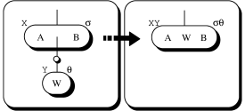
Figure 7: BEAM And-Compression rule.

This rule removes a nesting of two and-boxes by promoting the inner and-box to the outer and-box (see figure 7). It thus complements the promotion rule by allowing the BEAM to discard structure. The BEAM does not apply this rule if there is a pruning operator such as cut in the inner box (see section 3.2 for more details on pruning).

Doing and-compression has several benefits. First, the BEAM can recover memory immediately. Second, the compressed tree becomes smaller and easier to manage. Last, there is less information to duplicate when performing splitting.

3.1 Implicit Pruning

The BEAM implements two major simplifications that improve the search space by pruning logically redundant branches, even when they are not leftmost. The two rules are symmetrical: one is concerned with failed boxes, the other is concerned with successful boxes.

False-in-And

this simplification rule removes an and-box that is parent to a false box.

• $\displaystyle\hskip 25.00003pt{\begin{array}[]{lc}&\{\ldots\lor\Delta_{i\mathchar 45\relax 1}\lor[\exists{\mathcal{}X}:\sigma\makebox[0.6458pt]{}\&\makebox[0.6458pt]{}A\makebox[0.6458pt]{}\makebox[0.6458pt]{}\&\makebox[0.6458pt]{}\mathtt{false}\makebox[0.6458pt]{}\&\makebox[0.6458pt]{}B]\lor\Delta_{i\mathchar 43\relax 1}\lor\ldots\}\\ (False\mathchar 45\relax in\mathchar 45\relax And)&\longrightarrow\\ &\{\ldots\lor\Delta_{i\mathchar 45\relax 1}\lor\Delta_{i\mathchar 43\relax 1}\lor\ldots\}\end{array}}$

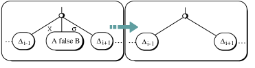
Figure 8: BEAM False-in-And simplification rule.

If a failure occurs at any point of the and-box, the and-box is removed and failure is propagated to the upper boxes (see figure 8). This rule can be considered a generalisation of the failure propagation strategies used in Independent And-Parallel systems [Hermenegildo and Nasr (1986)].

True-in-Or

This simplification rule removes an or-box that is parent to a true-box.

• $\displaystyle\hskip 25.00003pt{\begin{array}[]{lc}&[\exists{\mathcal{}X}:\sigma\makebox[0.6458pt]{}\&\makebox[0.6458pt]{}A\makebox[0.6458pt]{}\&\{\ldots\lor\makebox[0.6458pt]{}\mathtt{true}\makebox[0.6458pt]{}\lor\ldots\}\&\makebox[0.6458pt]{}B]\\ (True\mathchar 45\relax in\mathchar 45\relax Or)&\longrightarrow\\ &{[}\exists{\mathcal{}X}:\sigma\makebox[0.6458pt]{}\&\makebox[0.6458pt]{}A\makebox[0.6458pt]{}\&\makebox[0.6458pt]{}B]\end{array}}$

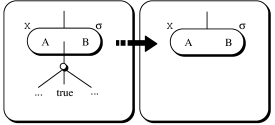
Figure 9: BEAM True-in-Or simplification rule.

This form provides implicit pruning of redundant branches in the search tree (see figure 9), and it generalizes XSB’s work on early completion of tabled computations [Sagonas (1996), Sagonas and Swift (1998)].

Implicit Pruning

These two rules can provide substantial pruning. In the absence of side effects, the presence of a true-box in a branch of an or-box should allow immediate pruning of all the other branches in the or-box. In an environment with side-effects, the user may still want the other branches to execute anyway. To guarantee Prolog compatibility, the BEAM by default only allows the true-in-or simplification and the false-in-and simplification for the leftmost goal. Alternatively, one could do compile-time analysis to disable the true-in-or and false-in-and optimization for the boxes where some branches include builtins calls with side-effects[Hermenegildo and Greene (1991), Santos Costa et al. (1991b)].

3.2 Explicit Pruning

The implicit pruning mechanisms we provide are not always sufficient for controlling the search space. The BEAM therefore supports two explicit pruning operators: cut (!) and commit ($|$) prune alternatives clauses for the current goal, plus alternatives for all goals created for the current clause. Cut only prunes branches that appear to the right of the current branch, commit can prune both to the left and to the right. Both operators disallow goals to their right from exporting constraints to the goals to the left, prior to execution. After the execution of a cut or commit, all and-boxes to the right of the and-box containing the cut operator are discarded and their constraints on external variables are promoted to the current and-box.

Figure 10 gives an example of explicit pruning for the program (we label the clauses of g/1 and h/1 to clarify the figure):

a(X) :- f(X), b(X).    f(X) :- g(X), !, h(X).
a(X) :- b(X).          f(X) :- i(X).

G1: g(1).              H1: h(3).
G2: g(2).              H2: h(2).

In this example the and-boxes for the sibling clause I and for the rightmost alternative G2 will be discarded. Next, the constraints for G1 can be promoted to the and-box for G, !, H.

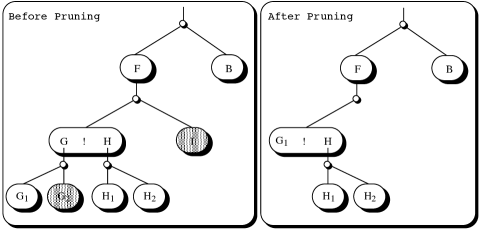
Figure 10: Cut scope.

The cut rule can be written as follows:

• $\displaystyle\hskip 25.00003pt{\begin{array}[]{lc}&\{[\exists{\mathcal{}X}:\theta_{1}\&\{[\exists{\mathcal{}Y}:\theta_{2}]\vee\ldots\}\&\makebox[0.6458pt]{}\mathtt{!}\makebox[0.6458pt]{}\&\makebox[0.6458pt]{}A]\vee\ldots\}\\ (Cut)\makebox[0.6458pt]{}\makebox[0.6458pt]{}\makebox[0.6458pt]{}\makebox[0.6458pt]{}\makebox[0.6458pt]{}\makebox[0.6458pt]{}\makebox[0.6458pt]{}\makebox[0.6458pt]{}\makebox[0.6458pt]{}\makebox[0.6458pt]{}\makebox[0.6458pt]{}\makebox[0.6458pt]{}\makebox[0.6458pt]{}\makebox[0.6458pt]{}&\longrightarrow\\ &\{[\exists{\mathcal{}X},{\mathcal{}Y}:\theta{{}_{1}}\theta{{}_{2}}\&A]\}\end{array}}$

and the commit rule as:

• $\displaystyle\hskip 25.00003pt{\begin{array}[]{lc}&\{\ldots\lor\makebox[0.6458pt]{}[\exists{\mathcal{}X}:\theta_{1}\&\{\ldots\vee[\exists Y:\theta_{2}]\vee\ldots\}\&\makebox[0.6458pt]{}\mathtt{|}\makebox[0.6458pt]{}\&\makebox[0.6458pt]{}A]\vee\ldots\}\\ (Commit)&\longrightarrow\\ &\{[\exists{\mathcal{}X},{\mathcal{}Y}:\theta{{}_{1}}\theta{{}_{2}}\&A]\}\end{array}}$

The conjunction of goals in the clause to the left of the cut or commit is called its guard. Our rule states that cut only applies when the goals in the guard have been unfolded into a configuration of the form:

• $\displaystyle\hskip 25.00003pt{\{[\exists{\mathcal{}X}:\theta_{2}]\vee\ldots\}}$

that is, when the leftmost branch of the guard has been completely resolved.

We next discuss in more detail the issues in the design of explicit pruning for the BEAM. In the following discussion we refer mainly to cut, but similar arguments apply to the commit operator.

4 Control for the BEAM

The previous rewrite and simplification rules provide the basic engine for the correct execution of logic programs. To this engine, we must add control strategies that decide which step to take and when. Describing when each rule is allowed to execute does not completely define the BEAM control strategy. It is also necessary to define the priority for each rule so that if a number of rewrite-rules match, one can decide which one to choose. Arguably, one could choose the same rule as Prolog, and clone Prolog execution. The real power of the EAM is that we have the flexibility to use different strategies. In particular, we will try to find one that minimises the search space. The key ideas are:

1. Failure propagation rules have priority over all the other rules, so that failure propagates as fast as possible.

2. Success propagation and and-compression rules should always be done next, because they simplify the tree.

3. Promotion and propagation rules should follow, because their combination may force some boxes to fail.

   The BEAM favors two types of reductions. First, deterministic reductions, do not create or-boxes, and thus will never lead to splitting. Second, reductions that do not constrain external variables can go ahead early.

4. Last, the splitting rule is the most expensive operation, and should be deferred as much as possible.

This default scheme of the execution control in BEAM thus favours deterministic rules: the simplification rules, the promotion rule and the propagation rule. Their implementation is therefore crucial to the system performance as we expect that most execution time in the EAM will be spent performing deterministic reductions, or reductions that do not constrain the external environment.

4.1 Improving Deterministic Work

Warren’s EAM proposal states that an and-box should immediately suspend when trying to non-deterministically constrain an external variable whose scope is above the closest or-box. Unfortunately, the original EAM rule may lead to difficulties. We next discuss two examples, a small data-base, parent/2, and a Prolog procedure, partition/4, given in Figure 11.

parent(john, richard).     partition([X|L],Y,[X|L1],L2) :- X =< Y,
parent(john, mary).                 partition(L,Y,L1,L2).
parent(patrick, paul).     partition([X|L],Y,L1,[X|L2]) :- X > Y,
parent(patrick, susan).             partition(L,Y,L1,L2).
                           partition([],_,[],[]).

Figure 11: Prolog’s parent/2 and partition/4 predicates.

Consider the query ?- parent(X,mary). The query is deterministic, as it only matches the second clause. Unfortunately, a naive implementation of Warren’s rule would not recognize the goal as deterministic. Instead, all four clauses would be tried, as parent/2 would try to bind a value to X, and all and-boxes would suspend.

The same problem may happen with the query: ?- partition([4,3,5],2,A,B). Although the calls are deterministic, the BEAM would suspend when unifying [X|L1] to A. The suspension would eventually lead to splitting and to poor performance.

AGENTS [Janson, Sverker (1994)] addresses this issue by relying on the guard operators to explicitly control when goals can execute. Arguably, this should allow for the best execution. On the other hand, AGENTS performance may be vulnerable to user errors, and Prolog programs need to be pre-processed in order to perform well [Bueno and Hermenegildo (1992)]. Andorra-I addresses a similar problem through its compiler. Unfortunately, coding all possible cases of determinacy grows exponentially [Palmer and Naish (1991)]. In the end, Andorra-I manages code size explosion by imposing a limit on the combinations of arguments that it tries [Santos Costa et al. (1991b)]. This solution becomes a source of inefficiency as Andorra-I often has to execute the same unifications twice: initially, when checking for determinacy, and later, after committing to a clause.

To address this problem, we propose a different control rule to define when a reduction should suspend. Reduction of an and-box cannot proceed and should therefore suspend if and only if:

1. unification of the head arguments constrains external variables, and,

2. at least two clauses unify with the current goal.

The BEAM performs full unification first and then checks whether these conditions hold. These provides a more aggressive determinacy scheme than the one in Warren’s EAM which leads to suspension immediately when binding an external variable. One advantage is that our scheme is simpler to implement, since the suspension may only occur at a fixed point of the code thus reducing the number of tests one needs to make in order to determine whether the current and-box should or should not suspend.

Condition (ii) assumes that we are able to detect which clauses may match. In practice this is the province of the indexing algorithm. It is known that detecting determinacy is in general NP-complete [Palmer and Naish (1991)]. Therefore, for efficiency reasons, the indexing algorithm will be a conservative approximation.

Deterministic-reduce-and-promote

Performance of many logic programs heavily depends on optimisations such as Last Call Optimisation. In the best case, such optimisations allow tail-recursive programs to execute with the same costs that iterative programs would.

Both EAM and AGENTS create an and-box when performing reduction on deterministic predicates. The newly created and-box is promoted immediately afterwards because it is deterministic. The creation of boxes that are immediately promoted is expensive, both in memory usage and in time.

The BEAM addresses this problem through the Deterministic-reduce-and-promote rule. This rule allows for a reduction to expand directly in the home and-box. More precisely, whenever a deterministic goal $B$ is to be reduced to a single alternative with goals $G_{1},\ldots,G_{n}$, the reduction can take place in the parent’s and-box. Figure 12 shows an example of this rule.

• $\displaystyle\hskip 25.00003pt{\begin{array}[]{lc}(Deterministic\mathchar 45\relax reduce&[\exists{\mathcal{}X}:\sigma\makebox[0.6458pt]{}\&\makebox[0.6458pt]{}A\makebox[0.6458pt]{}\&\makebox[0.6458pt]{}B\makebox[0.6458pt]{}\&\makebox[0.6458pt]{}C]\\ \makebox[0.6458pt]{}\mathchar 45\relax and\mathchar 45\relax promote)&\longrightarrow\\ &{[}\exists{\mathcal{}X},{\mathcal{}Y}:\sigma\theta\makebox[0.6458pt]{}\&\makebox[0.6458pt]{}A\makebox[0.6458pt]{}\&\makebox[0.6458pt]{}G_{1}\makebox[0.6458pt]{}\&\ldots\&\makebox[0.6458pt]{}G_{n}\makebox[0.6458pt]{}\&\makebox[0.6458pt]{}C]\end{array}}$

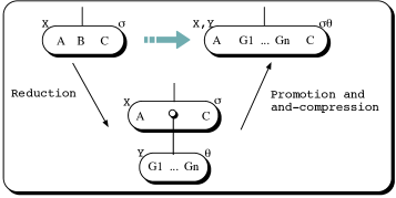
Figure 12: BEAM Deterministic-reduce-and-promote rule.

As explained before, the BEAM cannot apply the reduce-promote rule if there is a pruning operator, such as cut, in the inner and-box.

4.2 Control for Cut

Consider the example presented in Figure 13a, where the lower-leftmost and-box contains a cut (D,!,E). The and-box $W$ is the only box within the cut scope. Suppose that all boxes are suspended and that the only available rule is splitting. Unfortunately, splitting incorrectly allows the and-box $W$ to leave the scope of the cut (see figure 13c). An alternative would be to resort to Warren’s original forking rule, but forking incorrectly allows the and-box $C$ to be deleted by the cut (see figure 13b).

Please recall that the BEAM explicitly disallows the splitting of an and-box containing a cut. A clause with a cut can continue execution even if head unification constrains external variables (note that these bindings may not be made visible to the parent boxes). In this regard the BEAM is close to AGENTS [Janson, Sverker (1994)]. The BEAM differs from AGENTS in that goals to the right of the cut may also execute before pruning: the cut does not provide sequencing.

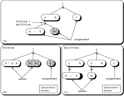
Figure 13: Incorrect use of Fork/Splitting and Cut.

Splitting can be applied freely whenever the goals within the guard of the cut do not constrain external variables, but it may not export constraints for variables external to the guard nor change the scope of the cut (see example in Figure 14).

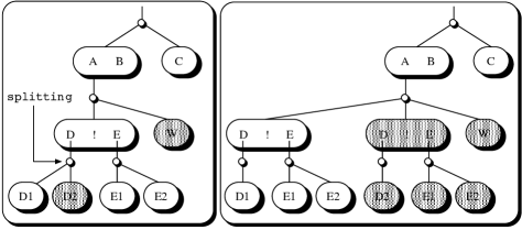
Figure 14: Correct use of splitting and cut.

The following two rules are used to control cut execution:

• Early-pruning - a cut can always execute immediately if it is the leftmost subgoal in the and-box and if the and-box does not have constraints.

  • $\displaystyle\hskip 25.00003pt{(Early\mathchar 45\relax pruning)\makebox[0.6458pt]{}\makebox[0.6458pt]{}\makebox[0.6458pt]{}\makebox[0.6458pt]{}\makebox[0.6458pt]{}\{[\exists{\mathcal{}Y}:\makebox[0.6458pt]{}\mathtt{!}\makebox[0.6458pt]{}\&\makebox[0.6458pt]{}\ldots]\vee W\}\longrightarrow\{[\exists{\mathcal{}Y}:\makebox[0.6458pt]{}\ldots]\}}$

  Consider the example illustrated in Figure 15a. Both alternatives to the goal a suspended trying to bind the external variable . The first alternative to the goal b contains a quiet cut  that will be allowed to execute since it respects the conditions described previously: the alternative does not impose external constraints, and the cut is the leftmost call in the and-box. Note that the resulting execution here is close to the standard Prolog execution.

  

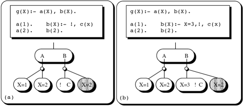
  Figure 15: Cut example.

  Figure 15b illustrates a different situation. In this case, the cut would not be allowed to execute since the alternative restricts the external variable X to the value 3. Thus, the computation in this example would only be allowed to continue after splitting on a. After splitting, the values 1 and 2 would be promoted to X and thus make the first alternative to b fail.

• Leftmost-pruning - if an and-box containing a cut becomes leftmost in the tree, the cut can execute immediately when all the calls before it succeed (even if there are external constraints).

  • $\displaystyle\hskip 25.00003pt{\begin{array}[]{lc}&[\exists{\mathcal{}X}_{1}:\theta_{1}\&\{\ldots\lor\{[\exists{\mathcal{}X}_{n}:\theta_{n}\&\mathtt{!}\&D]\vee W\}\lor\ldots\}\&E]\\ (Leftmost\mathchar 45\relax pruning)&\longrightarrow\\ &{[}\exists{\mathcal{}X}_{1}:\theta_{1}\&\{\ldots\lor\{[\exists{\mathcal{}X}_{n}:\theta_{n}\&D]\}\lor\ldots\}\&E]\end{array}}$

  For example, in Figure 16 the cut is allowed to execute immediately when X succeeds even if there are external constraints.

  

  Figure 16: Cut in the leftmost box in the tree.

Allowing early execution of cuts will in most cases prune alternatives early and thus reduce the search space.

Degenerate Parent Or-boxes

One interesting problem occurs when the parent or-box for the and-box containing the cut degenerates to a single alternative. In this case, promotion and and-compression would allow us to merge the two resulting and-boxes. As a result, cut could prune goals in the original parent and-box. Figure 17 shows an example where promotion of an and-box containing a cut leads to an incorrect state as the and-box C is in danger of being removed by cut.

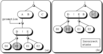
Figure 17: Incorrect use of promotion and cut.

The BEAM disallows and-compression when the inner and-box has a cut. Promotion of bindings is still allowed. Thus deterministic constraints are still allowed to be exported.

4.3 Non-Deterministic Work

Most programs have to perform splitting at some point. Deciding where to apply the splitting rule is a fundamental issue for EAM implementations. We have considered three major extensions to the default rule:

• Declare predicates as producers and allow them to perform Eager-Forking, that is, to do splitting as soon as they are called. The idea was first proposed by Gupta and Warren [Gupta and Warren (1991)]. Intuitively, we declare goals to be producers if we expect them to produce, but not consume, bindings from other goals.

  Eager-forking goes against the core idea of the EAM: doing determinate work first. On the other hand, it is simple to understand, it can increase parallelism, and in the cases where most alternatives in the producer fail quickly it can actually improve the search space. We have implemented eager-forking on the BEAM and we discuss some results in section 8.

• Allow the user to specify a boundary up to which we should check for splitting. The idea has appeared in many guises: mini-scopes in Gupta and Warren’s simulator [Gupta and Warren (1991)], independent computations in Bueno and Hermenegildo [Bueno and Hermenegildo (1992)]. Scoping is also quite important for a parallel implementation.

  AKL [Janson, Sverker (1994)] introduces stability to allow early splitting. If only splitting applies to an and-box $\Delta$, the and-box $\Delta$ is said to be stable if neither $\Delta$ nor any descendant and-box is suspended on variables external to $\Delta$. All stable and-boxes can be split in parallel. Unfortunately, detecting stability is quite expensive.

• The right-hand side of sequential conjunctions can be evaluated only after the left-hand-side has succeeded. We do not allow sequential conjunction below the default (parallel) conjunction. This is sufficient to guarantee correct ordering for side-effects builtins such as read/1 or write/1 [Santos Costa et al. (1991b)], and allows a simpler implementation.

In the next section we present the architecture used to implement BEAM, namely the And-Or Tree Manager and the Abstract Machine.

5 BEAM Implementation

Figure 18 illustrates the architecture organization for the BEAM execution model. The BEAM was implemented as an extension of the YAP Prolog system [Santos Costa (1999)]. It reuses most of the YAP compiler and its builtin library. The shadowed boxes show where the EAM stores data. The Code Space stores the data-base with the predicate/clause information, plus the bytecode to be interpreted by BEAM’s Abstract Machine Emulator (which we refer simply as Emulator). The Global Memory stores the And-Or Tree, and is further subdivided into the Heap and the Box Memory. The Box Memory stores dynamic data structures including boxes and variables. The Heap holds Prolog terms, such as lists and structures. The Heap uses term copying to store compound terms and is thus very similar to the WAM’s Heap.

There are a number of differences between the BEAM and the WAM. A major difference is that the BEAM does not perform backtracking. A Garbage Collector is thus necessary to recover space in the Heap. We leave the details on memory management to section 6.

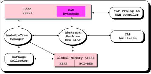
Figure 18: Execution Model.

The BEAM relies on two main components, shown as ovals in Fig. 18:

Emulator:

runs WAM-like code to perform unification and to setup boxes. Unification code is similar to the WAM. Control instructions follow a compilation scheme similar to the WAM but execute in a rather different way.

And-Or Tree Manager:

applies the BEAM rewriting rules to the existing and-boxes and or-boxes until WAM-like execution for the selected goal can start.

The And-Or Tree Manager handles most of the complexity in the EAM. It uses the Code Space area to determine how many alternatives a goal has and how many goals a clause calls. With this information the And-Or Tree Manager constructs the tree and uses the EAM rewriting rules to manipulate it. The Manager requests memory for the boxes from the Global Memory Areas. The Emulator is called by the And-Or Tree Manager in order to execute and unify the arguments of the goals and clauses. As an example consider the clause: p(X,Y):- g(X), f(Y). When running this clause the And-Or Tree Manager transforms p(X,Y) into an and-box, and calls the Emulator to create the subgoals and or-boxes for g(X) and f(Y). Control then moves to these subgoals, and will return to the And-Or Tree Manager only if the and-boxes generated for these subgoals need to suspend.

The details on how BEAM stores the And-Or Tree, the design of the Emulator and of the And-or Tree manager are described in more detail in the following sections.

5.1 Or-Boxes

Or-boxes represent open alternatives to a goal. Figure 19 presents the structure of an or-box. Each or-box refers to its parent and-box through the parent pointer, and to the sub-goal that created the or-box through the id_call field. The field nr_all_alternatives counts the number of current alternatives. Last, the box points to a list of alternatives, where each element in the list includes:

• a pointer to a corresponding and-box, alternative, initially null; it is initialized only when the alternative is explored;

• a pointer to the goal arguments, args; The first alternative creates the arguments vector. The last alternative to execute, after performing head unification, recovers the args vector as free memory. Each alternative needs a pointer to the args vector because the and-compression and the splitting rules can join alternatives to different goals;

• a pointer to the code for the alternative, code; and,

• the state of the alternative. Initially, alternatives are in the ready state. They next move to the running state, from where they may reach the success or fail states, or they may enter the suspend state. Suspended alternatives will eventually move to the wake state. From wake state alternatives move to the running state again. As an optimization, if no more sub-goals need to be executed, but the alternative is suspended, the alternative enters a special suspended_on_end state.

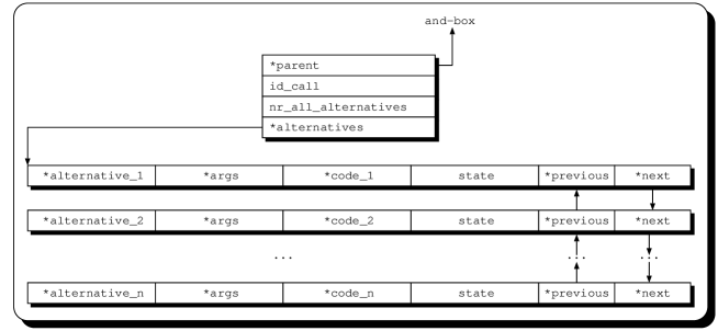
Figure 19: Or-Box representation.

Note that if nr_all_alternatives is one, then there is no need to keep the or-box: the determinate promotion rule can be applied to a single alternative. If nr_all_alternatives equals zero, the box has failed and we can perform fail propagation.

5.2 And-Boxes

And-boxes represent active clauses. And-boxes require a more complex structure than or-boxes, as they store information on which goals are active as well as on external and internal variables associated with the clause. Figure 20 shows an and-box.

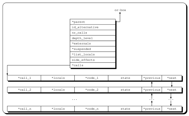
Figure 20: And-Box representation.

Access to the parent node is performed through the parent pointer and through the id_alternative field. The former points back to the parent or-box. The later indicates to which alternative the and-box belongs. Subgoal management requires knowing the number of subgoals in the clause, nr_calls. Each and-box maintains a depth_level counter that is used to classify variables. The locals field maintain a list of variables local to this and-box. Variable control is discussed in more detail in section 5.3. A list of bindings to external variables is accessed through the externals field. The and-box may have suspended trying to bind some variables, if so this is registered in the suspended field. If predicates with side-effects are present in the goals of this and-box, they are registered in the side_effects field. Last, each subgoal or call requires separate information:

• a pointer to a corresponding or-box, call, initially empty; it is initialized when the call is open;

• a pointer to the locals variables vector. Each goal needs an entry to the locals variables because the promotion and compression rules may add other goals and other variables to the and-box. Still, each goal needs to be able to identify its own local variables;

• a pointer to the code for the subgoal;

• State information says whether the goal is ready to enter execution, is running, or has entered the success or fail states. Goals may also be suspended or waiting on some variable, from which they will enter the wake state.

Initially each and-box has a fixed number of local variables. However, the number of local variables in an and-box may increase since the promotion rule allows one to promote local variables to a different and-box. We discuss local variables next.

5.3 Local Variables

Every variable is a local variable at some an-box; therefore it is represented through the structure illustrated in Figure 21. A local variable either belongs to a single subgoal in an and-box, or it is shared among subgoals. The value field stores the current working value for a variable. Unbound variables are represented as self-referencing pointers. Variables also maintain a list of and-boxes suspended on them, and point back to their home and-box.

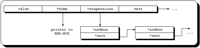
Figure 21: Local Variables representation used in the BEAM: note that suspensions are explained in detail in figure 23

The home field of a variable structure points directly to its original home and-box. However this field is not sufficient to completely determine if a variable is local or not to an and-box.

The BEAM detects whether a variable is local to an and-box or not by having each and-box associated with a depth-counter that is then used to classify variables. We can now recognize local variables as follows:

• A variable occurring in an and-box $\Delta$ is said to be local if the depth counter of the and-box $\Delta$ equals the depth counter of the variable’s home.

• Otherwise the variable is said to be external to the and-box $\Delta$.

5.4 External Variables

Each and-box maintains a list of External Variables, that is, of bindings for variables older than the current and-box (see Figure 22). Each such binding is represented as a data structure that includes a pointer to the variable definition, local_var, and to its new value, value. Whenever a goal binds an external variable, the assignment is recorded both in the current and-box as an external reference and at the local variable itself. This way, whenever a descendant and-box wants to use the value of the external reference, it can simply access the local variable. The external_reference data structure generalizes Prolog’s trail by allowing both the unwinding and the rewinding of bindings performed in the current and-box. Our scheme for the external variables representation is very similar to the forward trail [Warren (1984)] used in the SLG-WAM [Swift (1994), Sagonas and Swift (1998)].

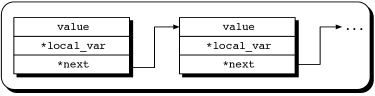
Figure 22: External variables representation.

5.5 Suspension List

The suspension list is a doubly linked list that keeps information on all suspended and-boxes (see figure 23). Each entry in the list maintains a pointer to the suspended and-box, and_box, and information on why the and-box suspended, reason. Goals may be suspended because they tried to bind external variables. They can also be waiting for an event to occur. For example, an I/O builtin may be waiting to be leftmost and an arithmetic builtin may be waiting for a variable to become bound.

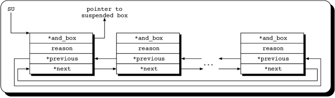
Figure 23: Suspension list representation.

The AGENTS implementation uses one stack for suspended boxes and another for woken boxes. In contrast, the BEAM uses the same list to maintain information on suspended and woken and-boxes. The SU pointer marks the beginning of the suspension list (that can be empty). Whenever an and-box suspends, an entry is added to the end of the suspension list. If a suspended and-box receives a wake signal, the and-box entry is moved to the beginning of the list. Thus, if there are woken boxes, they are immediately accessed by the SU pointer. Also note that we always want to work with woken boxes before working with the suspended ones. By default, the BEAM chooses the leftmost and-box in the And-Or Tree as the box to split first. The box is found by depth-first search.

6 Memory Management

The EAM implements a flexible control strategy. Memory usage can become a major concern in this case and the BEAM must carefully detect the points at which to recover space. As we show next, we have two techniques to recover space: we can reuse space for pruned boxes and we can garbage collect inaccessible data.

6.1 Reusing Space in the And-Or Tree

The Box Memory must satisfy intensive requests for the creation of and-boxes, or-boxes, local variables, external references, and suspension lists. Objects are small and most, but not all, will have short lifetimes. Objects are created very frequently and minimizing allocation and deallocation overheads is crucial.

Unfortunately, the BEAM cannot recover space through backtracking. Instead, it explicitly maintains liveness of data structures, and relies on a bucket allocation algorithm to allocate space.

The BEAM is therefore able to recover all memory from boxes whenever they fail or succeed. Memory from failed boxes can obviously be recovered since they do not add any knowledge to the computation. Memory from successful boxes can also be recovered because the variable unification rules guarantee that and-box variables do not reference variables within the subtree rooted at this box, that is, younger box variables can reference variables in upper boxes, but not the other way around, as described further in section 6.5.

We have chosen this scheme because it has a low overhead and most requests tend to vary among a relative small number of sizes[Lopes and Santos Costa (2005)].

6.2 Recovering Heap Space

The algorithm used to reuse memory space in the Box Memory will not work for the Prolog terms stored in the Heap because the BEAM releases memory eagerly, and the terms in the Heap tend to be very small, causing fragmentation and leaving only small blocks available. We could coalesce blocks to increase available block size [Detlefs et al. (1994)], but the price would be an increase in overheads. Instead, we have chosen to rely on a garbage collector to compact the Heap Memory.

We implemented a copying garbage collector [Jones and Lins (1996), Bevemyr and Lindgren (1994)] for the BEAM: live data structures are copied to a new memory area and the old memory area is released. The Heap memory is divided into two equal halves, growing in the same direction. The two halves could not grow in the opposite direction because the BEAM uses YAP builtins, and they expect the Heap to always grow upwards. Therefore we have a pre-defined limit-zone that, when reached, will activate the garbage collection mechanism by setting the garbage collector flag.

The garbage collection flag is periodically checked by the And-Or Tree manager to activate garbage collection. Thus, the garbage collector starts by replicating the living data in the root of the And-Or Tree and then follows a top-down-leftmost approach.

6.3 Variable Allocation

Variables are a major source of memory demand. In the initial implementation of the BEAM, all variables were processed the same way. Every and-box maintained a list of its local variables, and every variable would be in some and-box. Let us refer to these variables as permanent variables.

Processing all variables the same way has major drawbacks. Namely, during the execution of a program there is a large portion of memory that can be released only when the and-boxes fail or succeed.

The complexity of this variable implementation can also harm system performance. Consider one of the main rules of the EAM, Promotion, used to promote the variables and constraints from an and-box $\Delta$ to the nearest and-box $\Delta^{\prime}$ above. $\Delta$ must be a single alternative to the parent or-box, as shown in Fig. 2.

As in the original EAM promotion rule, promotion propagates results from a local computation to the level above. However, promotion in the BEAM does not merge the two and-boxes because the structure of the computation may be required to perform pruning as detailed in section 3.2  [Lopes et al. (2004)].

During the promotion of permanent variables, the home field of the variable structure needs to be updated so that it points to the new and-box $\Delta^{\prime}$. There is an overhead in this operation since one must go through the list of all permanent variables of $\Delta$. Moreover if $\Delta^{\prime}$ is promoted later, the system will have to go through $\Delta^{\prime}$ variables including all that it has inherited during promotions. With deterministic computations the list of permanent variables can grow very fast when promoting boxes, slowing down the BEAM.

6.4 Classification of Variables at Compile and Run-Time

Unfortunately, in general we do not know beforehand if we will need to suspend on a variable. We propose a WAM-inspired scheme, the BEAM-Lazy. Following the WAM, variables that appear only in the body of the clause or in queries are classified at compile time as permanent variables, meaning that all data-structures required for suspension are created for them. Otherwise, variables are classified at compile time as temporary.

As an example, consider the following clause of the nreverse procedure:

nreverse([X|L0],L) :- nreverse(L0,L1), concatenate(L1,[X],L).

In this clause, L1 is the only variable that is classified as permanent at compilation time. The other variables are classified as temporary. Thus, an and-box for this clause will have one permanent variable and three temporary variables. Still, it may need to create two more permanent variables, X and L0, when the clause is called with the first argument as variable (unify_var when writing terms).

Temporary variables require less memory and improve performance since we avoid managing the more complex structure of the permanent variables. A second advantage from using temporary variables is that they can be immediately released after executing the clause body, unlike permanent variables that can only be released when the and-box succeeds or fails. The BEAM implements tail-recursion in the presence of deterministic computation, so that temporary variables will be released before calling the last subgoal.

6.5 Variable Unification Rules

The main consideration in implementing a unification algorithm that supports both types of variables is that an and-box suspends only when trying to bind permanent variables external to the and-box.

There are three possible cases of variable-to-variable binding:

1. temporary variable to permanent variable: in this case the unification should make the temporary variable refer to the permanent variable. An immediate advantage is that the computation will not suspend. Unifying in the opposite direction would lead to an incorrect state.

2. temporary variable to temporary variable: the compiler ensures that a temporary variable is always bound to a permanent variable or a bound term, so this case will never occur.

3. permanent variable to permanent variable: the permanent variable that has its home box at a lower level of the tree should always reference the permanent variable that has its home box closer to the root of the tree.

   

   
   

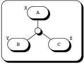
   Figure 24: Binding two permanent variables.

   Assume as an example the tree illustrated in figure 24 with three and-boxes: A, B, and C. Each box contains a single permanent variable: X,Y, and Z, respectively. Assume that the computation is processing the and-box B and that it becomes necessary to unify the variables X and Y. If the variable Y is made to reference the variable X, no suspension is necessary since the variable Y is local to the and-box B. Moreover, if the and-box B fails or if the computation continues to the and-box C no reset would be necessary in the variable X.

By following these unification rules one can often delay the suspension of an and-box and thus delay application of the expensive splitting rule.

7 The Emulator

The Emulator is responsible for running WAM-like code in order to perform unification and set up goals. The Emulator executes abstract machine instructions. The BEAM Emulator inherits most of the WAM instructions and WAM registers. However, new instructions and new registers are needed to cope with this rather different execution model.

7.1 Registers

In a fashion similar to the WAM, the BEAM internal state is saved in several registers:

• PC: Program Counter;

• H: Top of Heap;

• S: Structure pointer (points into the Heap);

• Mode: controls whether unification is in read or write mode;

• X1,X2,...: registers for temporary variables, also used as arguments registers;

• OBX: pointer to the working or-box.

• ABX: pointer to the working and-box.

• SU: pointer to the list of suspended and-boxes.

Note that, except for the last three, the registers are inherited from the WAM. On the other hand, several of the WAM registers, such as B, ENV, and HB, are not needed in the BEAM emulator as the BEAM does not implement backtracking. Instead information is stored directly in the And-Or Tree.

7.2 Abstract Machine Instructions

Code for the BEAM abstract machine very closely follows the WAM. The BEAM abstract machine instructions include the WAM get, put and unify instructions, plus some novel control instructions, that rely on the And-Or Tree Manager, described in section 7.3. The main control instructions are:

explore_alternative i:

explore the ith alternative for the current or-box. If there are more alternatives, create a new and-box. Otherwise, the parent and-box is reused for the alternative being executed (deterministic reduce and promote optimization). In both cases start executing the code for the unification of the arguments with the head of the goal.

prepare_calls n:

prepare the and-box to manage n subgoals. Each subgoal record points to the start code for the call, and is initialized as READY, meaning that they are ready to be explored. If the and-box does not have external variables, execution is then passed to the And-Or Tree Manager through next_call. Otherwise, the and-box is marked as suspended, and execution enters the And-Or Tree Manager through the suspend code.

call_pred n:

create one or-box with n branches, where n is the number of alternatives to pred. Each branch record points to the starting code of the corresponding alternative, and all branches are also initialized as READY, meaning that they are ready to be explored. Execution is then passed to the And-Or Tree Manager through the next_alternative code.

proceed:

return control from a clause to the Manager. If the and-box does not have external variables, it has succeeded, and enters the And-Or Tree Manager through the success module. Otherwise, the and-box is marked as suspended, and execution enters the And-Or Tree Manager through the suspend module.

The major difference between the BEAM’s get, put, and unify and the corresponding WAM instructions is that whenever one of these instructions tries to bind an external variable, an entry is added to the externals field on the current and-box. Note that in the WAM, during the unification of variables a check is also done to determine if trailing is necessary. Thus, the BEAM externals field can be viewed as similar to the WAM trailing mechanism.

7.2.1 Compilation

Compiling Prolog clauses to the BEAM abstract machine instructions is very similar to WAM compilation. Figure 25 illustrates an example of code generation.

         ancestor(X,Y):- parent(X,Y).
         ancestor(X,Z):- parent(X,Y), ancestor(Y,Z).

         parent(a,fa).
         parent(a,ma).
-------------------------------------------------------------
                          ancestor/2

    explore_alternative  1       |    explore_alternative  2
    get_var          A1,Y1       |    get_var          A1,Y3
    get_var          A2,Y2       |    get_var          A2,Y1
    prepare_calls     1 L1       |    prepare_calls  2 L1 L2
 L1:                             | L1:
    put_val          A1,Y1       |    put_val          A1,Y3
    put_val          A2,Y2       |    put_val          A2,Y2
    call_pred     parent/2       |    call_pred     parent/2
                                 | L2:
                                 |    put_val          A1,Y2
                                 |    put_val          A2,Y1
                                 |    call_pred   ancestor/2
-------------------------------------------------------------
                           parent/2

    explore_alternative  1       |    explore_alternative  2
    get_atom         A1, a       |    get_atom         A1, a
    get_atom         A2,fa       |    get_atom         A2,ma
    procceed                     |    procceed
                                 |
-------------------------------------------------------------

Figure 25: BEAM Abstract Machine Code for ancestor.

Note that, unlike in the WAM, code for rules in the BEAM does not end with an execute instruction. The BEAM abstract machine is goal based. As such, the explore_alternative i instruction initializes the ith or-branch by creating a new and-box in it. It is followed by a sequence of get instructions that perform the head unification. Next, if the clause is a fact, clause code terminates with the proceed instruction that decides whether the computation succeeds or whether it should suspend (i.e., there are constraints on external variables), entering the Manager through the success or the suspend modules respectively. If the clause is a rule, execution continues with the prepare_calls instruction. This instruction creates in the and-box as many subgoals as calls. Each subgoal is initialized to point to the start code of each call (marked as L1 and L2 in figure 25). Then, the prepare_calls jumps to the suspend module if there are constraints on external variables, or to the next_call port otherwise. Thus, it is up to the Manager to decide how and when to execute the calls. The caller code is composed of a series of put and possibly write instructions followed by the call_pred instruction. The call_pred instruction creates and initializes an or-box with as many branches as the number of valid alternatives (determined by the indexing on the first argument). Execution is then passed to the Manager through the next_alternative port that will decide which alternative to execute. By default, the leftmost alternative is chosen.

7.3 The And-Or Tree Manager

The And-Or Tree Manager is the heart of our system. Its task is to decide which rewrite rule should be applied to the current tree and then execute it. The computational tree contains and-boxes and or-boxes that can be in different states. The possible states for a box are:

• ready: when a box is ready to start execution;

• running: the box is already active and running;

• fail: the box has failed;

• success: the box has succeeded;

• suspended: the box is suspended at some point;

• suspended-on-end: the box is suspended and there are no more goals left to execute. This is a special case of suspended. The general case needs to continue the box execution. In this case we know that the execution is completed, so when the suspension is activated, the box can jump immediately to the success state.

• awoken: the box was suspended but has received a signal to be activated and can be restarted anytime.

The And-Or Tree Manager manages the states of and-boxes and decides when to move boxes from one state to another.

The And-Or Tree Manager is accessed through eight different entry points:

suspend:

this routine adds the current and-box to the suspension list. Next, the routine clears all assignments saved in the list of the external variables. Each external variable is also added to the suspension list included in the respective local variable. After that, the And-Or Tree Manager continues on next_alternative.

success:

this operation marks the current or-box as successful in its parent. The memory of the or-box is released. Next the parent and-box is checked. If all calls have reached success, space for the and-box is reclaimed and the operation is reentered for the upper or-box (Success Propagation). Otherwise, execution enters the next_call operation.

fail:

this routine marks the current and-box as failed in its parent. All the assignments made by the and-box are removed, and space for the and-box is reclaimed. If all the alternatives for the parent or-box have failed, the operation is recursively called for the parent and-box (Failure Propagation). Otherwise, if there is exactly one more alternative, execution moves to unique_alternative. If there are several alternatives, execution continues at next_alternative.

next_call:

this operation searches for the next non-suspended call in the current and-box. If there is a ready call in the current and-box, Reduction is applied by setting the PC to the start of the call’s code, and then execution jumps to the Emulator. Otherwise, if the and-box is not the root of the And-Or Tree, execution moves to next_alternative. If there is no ready call in the current and-box and if the current box is the root of the And-Or Tree, execution moves to the select_work operation.

next_alternative:

this routine searches for the next non-suspended alternative in the current or-box to continue with the Reduction of alternatives. If there is no such alternative, execution jumps to next_call. Otherwise, if the alternative is in the wake state, execution moves to the wake operation, else execution sets the PC to the code for the alternative code, and enters the Emulator.

unique_alternative:

this operation applies a promotion to the current and-box, since its parent or-box has a single alternative.

First, all external variables are checked, because after promotion some external variables may have become local. As a result, a wake signal is sent to all boxes suspended on this variable (propagation) that have their bindings promoted. If during the promotion of external variables unification fails, execution moves to the fail operation.

Second, if external variables still exist after the promotion, the and-box remains suspended, and execution moves to next_call. Otherwise, if the and-box is suspended and no more goals remain to execute, execution moves to success.

Last, if goals are still left to execute, the And-Or Tree Manager marks the and-box as running and continues its execution by entering the next_call operation.

wake:

this operation chooses a suspended and-box that has received a wake up signal (propagation).

First, all external variables are checked for changes: environment synchronization. The environment synchronization tests the compatibility of all the constraints imposed to external variables that are already bound. If unification fails, execution for the box jumps to fail. If unification succeeds for a variable, the and-box suspended on that variable can be deleted.

Last, If bindings to externals variables still exist, execution continues to select_work. If no more constraints on external variables are left, then the and-box enters suspended_on_end, and we can move immediately to success. Otherwise, execution marks the and-box as running and continues its execution by entering the next_call operation.

select_work:

this operation looks for work in the suspension list. If no extra work is available in the suspension list, execution will terminate. Otherwise, the ABX register is set to point to a box that is a candidate for splitting. By default, the BEAM splits the leftmost suspended box. After splitting, one of the resulting and-boxes is awakened, and its execution is restarted in wake.

7.3.1 The Interaction Between the And-Or Tree Manager and the Emulator

The And-Or Tree Manager interacts with the Emulator as illustrated in figure 26. In order to execute a query, the next_alternative first creates an or-box to store all possible alternative clauses. An alternative is then chosen and the execution passes to the Emulator, through the explore_alternative instruction. Following this, execution will run through a sequence of get and possibly some unify instructions that implement the unification of the head arguments. If this alternative is a fact then the emulator executes proceed. If there are assignments to external variables, this instruction will move execution to the And-Or Tree Manager suspend operation. Otherwise execution moves to the success operation.

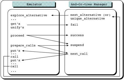
Figure 26: Connecting the And-Or Tree Manager with the Emulator.

If the alternative is a rule, then instead of proceed we have prepare_calls followed by a sequence of put and call_pred instructions. The prepare_calls instruction creates an and-box to store the calls and jumps to suspend if there are assignments to external variables in the and-box, or to next_call otherwise.

The next_call operation chooses a call to execute, by default the leftmost, and jumps to the Emulator where it executes the put instructions followed by a call_pred. The call_pred instruction will then jump to the next_alternative operation in order to repeat the entire process.

We have so far considered the straightforward execution case. Indeed, when running a normal program, the and-boxes will suspend when constraining external variables. Thus, a computational state with all and-boxes suspended is usual, and one must use the splitting rule (select_work) to create more deterministic work. The select_work operation selects a candidate to split (by default the leftmost suspended and-box). After splitting, the computation can restart by waking one of the resulting and-boxes. The wake operation will then perform an environment check to determine if the constraints being promoted are compatible with (possible) constraints imposed by other and-boxes.

8 Performance Analysis

In this section we present the performance results of the prototype BEAM system. For the analysis of the BEAM performance we compare it with the following systems:

• SICStus Prolog 3.12.0 [I.S.Laboratory (2004)]: is a state-of-the-art, ISO standard compliant, Prolog system developed at the SICS (the Swedish Institute of Computer Science). It is a commercial widely known system. All benchmarks were executed using compiled emulated code.

• YAP 5.0 [Santos Costa (1999)]: is another state-of-the-art emulated Prolog system that was developed at University of Porto. This system is often regarded as the fastest Prolog system available for the PC Platform.

• YAP 4.2: is an older version of the YAP Prolog. BEAM was implemented on top of it.

• Andorra-I v1.14 [Santos Costa (1993)]: is an implementation of the Basic Andorra Model that exploits or-parallelism and determinate dependent and-parallelism while fully supporting Prolog. We have used the sequential version for the comparison. All benchmarks were pre-compiled by the Andorra-I preprocessor before execution.

• AKL AGENTS v1.0 [Janson and Montelius (1992)]: is a sequential Andorra Kernel Language implementation. The language was designed by Sverker Janson and Seif Haridi. AGENTS was developed by Johan Bevemyr and others, at SICS, Sweden. This system follows an execution scheme that is similar to BEAM’s but has the control intrinsic in the language. All benchmarks were rewritten to the AKL language before compiling and executing them on the Agents system.

We have used a representative group of well-known benchmarks. For each benchmark we present the best execution time from a series of ten runs. The runtime is presented for all systems in milliseconds. Smaller benchmarks were run repeatedly. The timings were measured running the benchmarks on an Intel Pentium Mobile 1800Mhz (533Mhz FSB) with 2MB on chip cache, equipped with 1GB at 333Mhz DDR SDRAM and running Fedora Core 3. The BEAM was configured with 64MB of Heap plus 32MB of Box Memory. Benchmark code is available at http://www.dcc.fc.up.pt/~fds/rslopes.

8.1 The Benchmark Programs

Table 1 gives a small description of the benchmarks used in this section. The selected group of benchmarks is composed by well known test programs used within the Prolog community.

Table 1: The benchmarks.

Deterministic:
cal	last 10000 FoolsDays arithmetic benchmark.
deriv	symbolically differentiates four functions of a single variable.
qsort	quick-sort of a 50-element list using difference lists.
serialise	calculate serial numbers of a list.
reverse	smart reverse of a 1000-element list.
nreverse	naive reverse of a 1000-element list.
kkqueens	smart finder of the solutions for the n-queens problem.
tak	heavily recursive with lots of simple integer arithmetic.
Non-Deterministic:
ancestor	query a static database.
houses	logical puzzle based on constraints.
query	finds countries with approximately equal population density.
zebra	logical puzzle based on constraints.
puzzle4x4	finds a solution for a quadratic puzzle.
send	the SEND+MORE=MONEY puzzle.
scanner	a program to reveal the content of a box.
queens	finds safe placements of $n$-queens on $n*n$ chessboard.
check_list	list checker that verifies if duplicate elements exist.
ppuzzle	naive generation and test valid paths in a quadratic puzzle.

The benchmarks are divided into two classes: deterministic and non-deterministic. The non-deterministic benchmarks are further subdivided into two groups: benchmarks that do not benefit from the Andorra rule and benchmarks where the Andorra rule allows the search space to be reduced.

8.2 Performance on Deterministic Applications

Table 2 shows how the BEAM performs versus Andorra-I, AGENTS, and the Prolog systems for deterministic applications. We use SICStus Prolog as the reference system, so we give actual execution times for SICStus and the relative time for the other systems. Neither the BEAM nor AGENTS perform splitting, and Andorra-I always executes deterministically. Prolog systems may create choice points.

Table 2: Deterministic benchmarks. SICStus Prolog is used as the reference system, with time given in milliseconds.

	SICStus				YAP
Benchs.	3.12	BEAM	AGENTS	Andorra-I	4.2	5.0
cal	0.001	29%	20%	20%	48%	143%
deriv	0.010	31%	8%	33%	72%	128%
qsort	0.045	23%	14%	24%	88%	102%
serialise	0.030	27%	15%	15%	103%	107%
reverse_1000	0.050	27%	12%	15%	42%	116%
nreverse_1000	23	23%	11%	23%	115%	153%
kkqueens	30	27%	20%	20%	58%	158%
tak	16	31%	33%	23%	160%	133%
average		27%	17%	22%	86%	130%

The YAP and SICStus Prolog systems are recognized as some of the fastest Prolog systems on the x86 architectures. The difference between Yap4.2 (on which the BEAM is based) and Yap5 shows that there is scope for improvement even for Prolog systems. These improvements should also benefit the BEAM. Comparing with the BEAM, Yap5 is about 5 times faster than the BEAM. SICStus Prolog and Yap4.2 are a bit less fast. This is quite a good result for the BEAM, considering the extra complexity of the Extended Andorra Model.

The BEAM tends to perform better than the AGENTS especially on tail-recursive computations. We believe this is because the BEAM has special rules for performing tail-recursive computation that avoid creating intermediate or-boxes and and-boxes. The results are especially good for the BEAM considering that the BEAM does not need any explicit control on these benchmarks. On the other hand, AGENTS benefits from extra control to run the benchmarks deterministically.

Performance of the BEAM is very close to the performance of Andorra-I. Andorra-I beats BEAM on two benchmarks: deriv and qsort. This seems to depend on determinacy detection performed by the Andorra-I preprocessor. Consider the following code from the qsort benchmark:

   partition([X|L],Y,[X|L1],L2) :- X =< Y, partition(L,Y,L1,L2).
   partition([X|L],Y,L1,[X|L2]) :- X  > Y, partition(L,Y,L1,L2).

Andorra-I classifies this code as deterministic, and never creates a choice point. Unlike Andorra-I, BEAM does not have a pre-compilation with determinacy analysis to classify this predicate as deterministic. Thus, the sophisticated determinacy code in Andorra-I can limit the overheads that the BEAM has to go through by creating unnecessary and-boxes. For better understanding these overheads that BEAM suffers from, consider the two possible cases when running the partition predicate:

• X $\leq$ Y: the BEAM creates an or-box with two alternatives. It performs the head unification for the first alternative and it succeeds executing the test comparing X with Y. Execution then immediately suspends, because head unification generates bindings to variables external to the box. Execution then continues with the second alternative that will fail when comparing X to Y. This failure makes the first alternative the unique alternative in the or-box, and a promotion will occur allowing the suspended computation to resume.

• X $\mathchar 62\relax$ Y: the BEAM creates an or-box with two alternatives. The first alternative will fail when comparing X and Y. This failure makes the second alternative unique in its or-box. Promotion thus will occur, allowing the second alternative to run deterministically without suspending.

Concluding, the BEAM deterministic performance seems to be somewhat better than AGENTS and equivalent to Andorra-I, although in some code the BEAM still has greater overheads than Andorra-I.

8.3 Performance on Non-Deterministic Applications

Comparing different systems for non-deterministic benchmarks is hard, since the search spaces may be quite different for Prolog, BEAM, AGENTS, and Andorra-I. We will consider two classes of non-deterministic applications. First, we consider applications where the Andorra Model does not provide improve the search space. Note that in general one would not be particularly interested in the BEAM for these applications: first, splitting is very expensive and second, or-parallelism can also be quite effectively exploited in Prolog. Next, we will consider examples where the Andorra rule reduces, very significantly, the search space.

Table 3 shows a set of five non-deterministic benchmarks. Again, we use SICStus Prolog as the reference system. The number of splits for the BEAM and AGENTS and the number of non-deterministic steps for Andorra-I for this set of benchmarks is presented in table 4. We consider two versions of the BEAM. The default version delays splitting until no other rules are applied. The ES version uses eager splitting. In this version splitting on producer goals is performed immediately. Producer goals are identified through the use of an annotation inserted in the Prolog program. Eager splitting makes the BEAM computation rule closer to that of Prolog. Note that to attain good results with eager splitting, BEAM depends on the user to identify the producer goals. Ideally, we would prefer to use compile time analysis instead.

Table 3: Non-deterministic benchmarks. SICStus Prolog is used as the reference system with time given in milliseconds.

	SICStus	BEAM				YAP
Benchs.	3.12	Default	ES	AGENTS	AND.-I	4.2	5.0
ancestor	0.014	N/A	38%	6%	16%	139%	152%
houses	0.37	79%	82%	86%	46%	132%	206%
query	0.30	3%	12%	2%	29%	85%	236%
zebra	7.50	33%	79%	40%	32%	97%	124%
puzzle4x4	200	32%	N/A	23%	22%	101%	121%
average		37%	53%	32%	29%	111%	168%

Table 4: Number of splits for BEAM/AGENTS and non-deterministic steps for Andorra-I.

	BEAM
Benchs.	Default	ES	AGENTS	ANDORRA-I
ancestor	N/A	30	73	75
houses	49	68	236	237
query	624	624	624	626
zebra	695	294	493	3,631
puzzle4x4	53,350	N/A	53,350	53,351

This set of benchmarks covers several major cases that can occur when using eager splitting on BEAM.

• The ancestor benchmark [Gupta and Warren (1991)], is one example where having producers avoids a situation where the EAM may loop.

• The houses benchmark is an interesting case where, although eager splitting increases the number of splits, performance still has a slight improvement. This example shows that splitting earlier with less data to copy may have advantages in some cases. Moreover, the BEAM has a lower number of splits than AGENTS because the BEAM can delay splitting until success or failure propagation, whereas AGENTS depends on guards.

• Using eager splitting on the query benchmark does not change the number of splits performed but has a huge improvement on system performance.

• The zebra benchmark is another demonstration of the impact of eager-splitting in the EAM. In this example just defining the producer dramatically cuts the search space and achieves much better performance than AGENTS and Andorra-I. Moreover, the good execution time when compared with Prolog indicates that the system actually reduces the search space.

• Finally, in the puzzle benchmark the main goal suspends during the head unification and is forced to perform splitting immediately. Thus, there is no early execution, and no difference in using eager splitting.

To better understand the effects of the splitting rule, and what implications eager splitting can have on the computation tree, consider the example illustrated in figure 27.

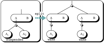
Figure 27: Splitting effects.

We assume two goals, the producer A and the consumer B. The BEAM allows two methods to determine when to split on the goal A:

• default rule: the split on A will only be performed when all the computation on B suspends. If A is a producer, then there is a risk of having the EAM create speculative work on B (in the worst case even leading to non-termination). Moreover, when splitting on A, the entire And-Or Tree created on B will be copied. This copying can be expensive and bring a large penalty to the execution time.

• with eager splitting on A: the split on A will be performed before starting execution of B. The split will be simpler since there will be no data associated with the goal B to replicate. The disadvantage is that this goal after the splitting is totally unexplored in two and-boxes of the tree, and thus there is duplication of work.

In general, eager splitting is appropriate when we expect that early execution of the other goals will not constrain the producers. In other words, early splitting should be pursued if we expect splitting to be needed anyway. In that case, early splitting makes splitting much less expensive.

8.3.1 Improving the Search Space

The main benefit of the BEAM is in applications where we can significantly improve the search space. Such applications may be pure logic programs, or may be applications that take advantage of the concurrency inherent to the Andorra Model. We consider five examples. The send_more_money and the scanner benchmarks are well-known examples of declarative programs that perform badly in Prolog. A set of Prolog benchmarks would not be complete without experimenting with a naive solution to find the first solution for the queens problem. And finally we consider two benchmarks that process lists, the check_list and the ppuzzle. Each list element is a pair with the form $p(X,Y)$ representing a position in an $n*n$ matrix. The check_list benchmark succeeds if an input list does not hold duplicate elements. The ppuzzle generates all lists with all possible combinations of the different elements in an $n*n$ matrix, and validates those that obey certain predefined conditions.

Results are shown in table 5 and table 6. The send-more-money, the scanner and the queens benchmarks are quite interesting because the BEAM without extra controls does not perform more splits than AGENTS and it has slightly better performance. Performance is three orders of magnitude faster than Prolog’s. These benchmarks are also interesting in that they show a situation where the more Prolog-like Andorra-I actually obtains the best results. Although performing the same (or a few more) non-deterministic steps as BEAM and AGENTS, Andorra-I is faster as choice-point manipulation is more efficient than splitting.

Table 5: Reduced search benchmarks (time in milliseconds).

Benchs.	BEAM	AGENTS	ANDORRA-I	YAP 5.0
send_money	7	8	0.8	7,767
scanner	20	39	3	$\mathchar 62\relax$12 hours
queens-9	2	8	0.9	16
queens-10	11	27	2.2	124
queens-11	7	19	1.3	893
queens-12	45	109	6.4	9,042
queens-13	23	58	3.4	93,343
queens-14	523	1,122	60	1,175,535
queens-15	456	1,042	50	15,287,308
queens-16	3,958	8,363	396	$\mathchar 62\relax$12 hours
queens-17	2,547	5,847	230	$\mathchar 62\relax$12 hours
queens-18	21,891	47,113	1,890	$\mathchar 62\relax$12 hours
queens-19	1,572	3,796	120	$\mathchar 62\relax$12 hours
queens-20	138,799	302,048	10,680	$\mathchar 62\relax$12 hours
check_list-8	0.05	0.06	1,150	183
check_list-9	0.07	0.07	5,810	963
check_list-10	0.09	0.09	209,140	34,910
check_list-11	0.10	0.11	6,165,824	987,243
check_list-15	0.17	0.18	$\mathchar 62\relax$12 hours	$\mathchar 62\relax$12 hours
ppuzzle-A	8	5	134,417	$\mathchar 62\relax$12 hours
ppuzzle-B	18	10	$\mathchar 62\relax$12 hours	$\mathchar 62\relax$12 hours
ppuzzle-C 1st	1.9	1.3	2,059,329	$\mathchar 62\relax$12 hours

Table 6: Number of splits for BEAM/AGENTS and non-deterministic steps for Andorra-I.

Benchs.	BEAM	AGENTS	ANDORRA-I
send_money	277	277	325
scanner	310	440	75
queens-9	129	129	130
queens-10	364	364	364
queens-11	212	212	212
queens-12	1,109	1,109	1,110
queens-13	522	522	523
queens-14	9,046	9,046	9,046
queens-15	7,054	7,054	7,055
queens-16	52,617	52,617	52,617
queens-17	31,210	31,210	31,210
queens-18	236,172	236,172	236,173
queens-19	16,178	16,178	16,178
queens-20	1,229,355	1,229,355	1,229,355
check_list-8	1	19	525,447
check_list-9	1	22	2,658,697
check_list-10	1	26	95,365,524
check_list-11	1	32	-
check_list-15	1	64	-
ppuzzle-A	86	86	64,994,853
ppuzzle-B	215	215	-
ppuzzle-C 1st	29	29	751,567,244

The check_list and the ppuzzle benchmarks are examples where the EAM benefits from allowing non-deterministic goals to execute as long as they do not bind external variables, as these goals actually fail early. On the other hand, Andorra-I is limited on this benchmark by the non-determinism of the main predicates. On check_list Andorra-I has a search space similar to Prolog’s, while in the ppuzzle Andorra-I is better than Prolog, but still has a larger search space than BEAM and AGENTS. The difference seems to be that both the BEAM and AGENTS benefit from early execution of the body of rules.

9 Conclusions & Related work

We have presented the design and the implementation of the BEAM, a system for the efficient execution of logic programs based on David H. D. Warren’s work on the Extended Andorra Model with implicit control. Our work was motivated by our interest in studying how the EAM with implicit control can be effectively implemented and how it can perform versus other execution strategies. We believe the BEAM is a step towards extending logic programming for applications where Prolog currently does not perform well. We believe that our results are quite encouraging in this direction.

Our approach contrasts with previous work in concurrent languages such as AKL. These are powerful concurrent languages that open up new programming paradigms, but that also require users to invest in sophisticated new programming frameworks. In contrast, our first goal is to support a very flexible engine for the execution of logic programs. The engine can then be controlled through several control primitives.

The main contribution of this work is thus the design and implementation of the BEAM. Further, our work in clarifying the EAM and in designing the BEAM has shown a crisp separation between the rewrite rules and control. We have tried to make this separation clear in this presentation.

In the future, we would like to explore different control strategies over the basic rewrite-rules. Indeed control may be made configurable, say, by using a specialized control language that can generate specialized And-Or Tree managers. We believe that a major contribution of the EAM is the exciting prospect of achieving specialized control strategies for different types of logic programs.

The current BEAM prototype is available as part of the YAP Prolog system distribution since release 5.1 [Santos Costa (2008)]. Although the BEAM is still a prototype, results are promising. The BEAM appears as an alternative to run programs where standard Prolog systems behave badly. Unlike AGENTS, the BEAM supports Prolog and unlike Andorra-I it does not need pre-compilation analysis. Thus, the BEAM is an excellent alternative for applications where pre-compilation to Prolog may be expensive and difficult and where queries with large search spaces are generated in rapid succession.

The BEAM prototype is currently being ported to the latest version of YAP, with the new indexing algorithm [Santos Costa et al. (2007)], which should further improve BEAM performance. Currently, the BEAM only supports Herbrand domain constraints. We plan to use YAP attributed variable support to exloit non-Herbrand constraints. Ultimately, we aim at making the BEAM an extension of Prolog systems that the user can exploit towards maximum performance in declarative applications.

We believe that the BEAM provides an excellent framework for novel logic programming applications. We are particularly interested in performance evaluation for automatically generated queries, say, the ones that are found in Inductive Logic Programming [Santos Costa et al. (2003)]. In these applications, queries with large search spaces are generated in rapid succession. Reducing the search space is fundamental, but pre-compilation to Prolog may be expensive and difficult. We believe that the advanced search features of the EAM can be most useful for these applications.

Acknowledgments

We would like to gratefully acknowledge the contributions we received from Salvador Abreu, Gopal Gupta, Enrico Pontelli and Ricardo Rocha. The work presented in this paper has been partially supported by project HORUS (PTDC/EIA-EIA/100897/2008), LEAP (PTDC/EIA-CCO/112158/2009), and funds granted to LIACC and CRACS & INESC-Porto LA through the Programa de Financiamento Plurianual, Fundação para a Ciência e Tecnologia and Programa POSI. Last, but not least, we would like to gratefully acknowledge the anonymous referees for the major contributions that they have given to this paper.

References

- Aggoun et al. (1995) Aggoun, A., Chan, D., Dufresne, P., Falvey, E., Grant, H., Herold, A., Macartney, G., Meier, M., Miller, D., Mudambi, S., Perez, B., van Rossum, E., Schimpf, J., Tsahageas, P. A., and de Villeneuve, D. H. 1995. ECLiPSe 3.5 User Manual. ECRC.
- Bevemyr and Lindgren (1994) Bevemyr, J. and Lindgren, T. 1994. A simple and efficient copying garbage collector for Prolog. In 6th International Symposium on Programming Language Implementation and Logic Programming, PLILP’94. LNCS, vol. 844. Springer-Verlag, 88–101.
- Bueno and Hermenegildo (1992) Bueno, F. and Hermenegildo, M. V. 1992. An Automatic Translations Scheme from Prolog to the Andorra Kernel Language. In International Conference on Fifth Generation Computer Systems 1992. ICOT, Tokyo, Japan, 759–769.
- Colmerauer (1993) Colmerauer, A. 1993. The Birth of Prolog. In The Second ACM-SIGPLAN History of Programming Languages Conference. ACM, 37–52.
- Detlefs et al. (1994) Detlefs, D., Dosser, A., and Zorn, B. 1994. Memory allocation costs in large C and C++ programs. Softw. Pract. Exper. 24, 6, 527–542.
- Gupta and Pontelli (1997) Gupta, G. and Pontelli, E. 1997. Extended dynamic dependent And-parallelism in ACE. In PASCO ’97. Proceedings of the second international symposium on parallel symbolic computation, July 20–22, 1997, Maui, HI, ACM, Ed. ACM Press, New York, NY 10036, USA, 68–79.
- Gupta et al. (2001) Gupta, G., Pontelli, E., Ali, K., Carlsson, M., and Hermenegildo, M. 2001. Parallel Execution of Prolog Programs: A Survey. ACM Transactions on Programming Languages and Systems 23, 4, 1–131.
- Gupta and Warren (1991) Gupta, G. and Warren, D. H. D. 1991. An Interpreter for the Extended Andorra Model. Internal report, University of Bristol.
- Hermenegildo and Greene (1991) Hermenegildo, M. V. and Greene, K. 1991. &-Prolog and its Performance: Exploiting Independent And-Parallelism. New Generation Computing 9, 3,4, 233–257.
- Hermenegildo and Nasr (1986) Hermenegildo, M. V. and Nasr, R. I. 1986. Efficient Management of Backtracking in AND-parallelism. In Third International Conference on Logic Programming. Number 225 in Lecture Notes in Computer Science. Imperial College, Springer-Verlag, 40–54.
- Hill (1974) Hill, R. 1974. LUSH-Resolution and its Completeness. Dcl memo 78, Department of Artificial Intelligence, University of Edinburgh.
- I.S.Laboratory (2004) I.S.Laboratory. 2004. SICStus Prolog user’s manual, 3.12.0 Technical Report. Swedish Institute of Computer Science.
- Janson and Haridi (1991) Janson, S. and Haridi, S. 1991. Programming Paradigms of the Andorra Kernel Language. In International Logic Programming Symposium, ILPS’91. MIT Press, 167–186.
- Janson and Montelius (1992) Janson, S. and Montelius, J. 1992. Design of a Sequential Prototype Implementation of the Andorra Kernel Language. SICS Research Report, Swedish Institute of Computer Science.
- Janson, Sverker (1994) Janson, Sverker. 1994. AKL – A Multiparadigm Programming Language. Ph.D. thesis, Uppsala University.
- Jones and Lins (1996) Jones, R. and Lins, R. 1996. Garbage Collection: Algorithms for Automatic Dynamic Memory Management. John Wiley and Sons. Reprinted February 1997.
- Lloyd (1987) Lloyd, J. W. 1987. Foundations of Logic Programming, second ed. Springer-Verlag.
- Lopes and Santos Costa (2005) Lopes, R. and Santos Costa, V. 2005. Improving memory usage in the beam. In 7th International Symposium on Pratical Aspects of Declarative Languages, PADL’05, M. Hermenegildo and D. Cabeza, Eds. LNCS, vol. 3350. Springer-Verlag, 143–157.
- Lopes et al. (2001) Lopes, R., Santos Costa, V., and Silva, F. 2001. A novel implementation of the extended andorra model. In 3rd International Symposium on Pratical Aspects of Declarative Languages, PADL’01, I. V. Ramakrishnan, Ed. LNCS, vol. 1990. Springer-Verlag, 199–213.
- Lopes et al. (2003a) Lopes, R., Santos Costa, V., and Silva, F. 2003a. On deterministic computations in the extended andorra model. In 19th International Conference on Logic Programming, ICLP03, C. Palamidessi, Ed. LNCS, vol. 2916. Springer-Verlag, 407–421.
- Lopes et al. (2003b) Lopes, R., Santos Costa, V., and Silva, F. 2003b. On the beam implementation. In 11th Portuguese Conference on Artificial Intelligence, EPIA 2003, F. M. Pires and S. Abreu, Eds. LNCS, vol. 2902. Springer-Verlag, 131–135.
- Lopes et al. (2004) Lopes, R., Santos Costa, V., and Silva, F. 2004. Prunning in the extended andorra model. In 6th International Symposium on Pratical Aspects of Declarative Languages, PADL’04, B. Jayaraman, Ed. LNCS, vol. 3057. Springer-Verlag, 120–134.
- Montelius and Ali (1995) Montelius, J. and Ali, K. A. M. 1995. An And/Or-Parallel Implementation of AKL. New Generation Computing 13, 4, 31–52.
- Montelius and Magnusson (1997) Montelius, J. and Magnusson, P. 1997. Using SIMICS to evaluate the Penny system. In International Logic Programming Symposium, ILPS’97, J. Małuszyński, Ed. MIT Press, Cambridge, 133–148.
- Palmer and Naish (1991) Palmer, D. and Naish, L. 1991. NUA-Prolog: an Extension to the WAM for Parallel Andorra. In 8th International Conference on Logic Programming, ICLP’91, K. Furukawa, Ed. MIT Press.
- Sagonas (1996) Sagonas, K. 1996. The SLG-WAM: A Search-Efficient Engine for Well-Founded Evaluation of Normal Logic Programs. Ph.D. thesis, Department of Computer Science, State University of New York, Stony Brook, USA.
- Sagonas and Swift (1998) Sagonas, K. and Swift, T. 1998. An Abstract Machine for Tabled Execution of Fixed-Order Stratified Logic Programs. ACM Transactions on Programming Languages and Systems 20, 3 (May), 586–634.
- Sagonas et al. (1997) Sagonas, K., Swift, T., Warren, D. S., Freire, J., and Rao, P. 1997. The XSB programmer’s manual. Tech. rep., State University of New York at Stony Brook. Available at http://www.cs.sunysb.edu/~sbprolog.
- Santos Costa (1993) Santos Costa, V. 1993. Compile-Time Analysis for the Parallel Execution of Logic Programs in Andorra-I. Ph.D. thesis, University of Bristol.
- Santos Costa (1999) Santos Costa, V. 1999. Optimising Bytecode Emulation for Prolog. In International Conference Principles and Practice of Declarative Programming, PPDP’99. Springer-Verlag, LNCS 1702, 261–267.
- Santos Costa (2008) Santos Costa, V. 2008. The life of a logic programming system. In 24th International Conference on Logic Programming, ICLP 2008, M. G. de la Banda and E. Pontelli, Eds. LNCS, vol. 5366. Springer-Verlag, 1–6.
- Santos Costa et al. (2000) Santos Costa, V., Damas, L., Reis, R., and Azevedo, R. 2000. YAP User’s Manual. Universidade do Porto. available at http://www.dcc.fc.up.pt/~vsc/Yap.
- Santos Costa et al. (2007) Santos Costa, V., Sagonas, K., and Lopes, R. 2007. Demand-driven indexing of prolog clauses. In 23rd International Conference on Logic Programming, ICLP’07, V. Dahl and I. Niemelä, Eds. LNCS, vol. 4670. Springer, 305–409.
- Santos Costa et al. (2003) Santos Costa, V., Srinivasan, A., Camacho, R., Blockeel, H., Demoen, B., Janssens, G., Struyf, J., Vandecasteele, H., and Van Laer, W. 2003. Query Transformations for Improving the Efficiency of ILP Systems. Journal of Machine Learning Research 4, 465–491.
- Santos Costa et al. (1991a) Santos Costa, V., Warren, D. H. D., and Yang, R. 1991a. Andorra-I: A Parallel Prolog System that Transparently Exploits both And- and Or-Parallelism. In 3rd ACM SIGPLAN Symposium on Principles & Practice of Parallel Programming, PPOPP’91. ACM press, 83–93. SIGPLAN Notices vol 26(7), July 1991.
- Santos Costa et al. (1991b) Santos Costa, V., Warren, D. H. D., and Yang, R. 1991b. The Andorra-I Preprocessor: Supporting full Prolog on the Basic Andorra model. In 8th International Conference on Logic Programming, ICLP’91. MIT Press, 443–456.
- Smolka (1995) Smolka, G. 1995. The Oz programming model. In Computer Science Today, J. van Leeuwen, Ed. LNCS, vol. 1000. Springer-Verlag, Berlin, 324–343.
- Swift (1994) Swift, T. 1994. Efficient Evaluation of Normal Logic Programs. Ph.D. thesis, Department of Computer Science, State University of New York, Stony Brook, USA.
- Ueda (2002) Ueda, K. 2002. A Pure Meta-interpreter for Flat GHC, a Concurrent Constraint Language. In Computational Logic: Logic Programming and Beyond. LNCS, vol. 2407. Springer, 138–161.
- Ueda and Morita (1990) Ueda, K. and Morita, M. 1990. A New Implementation Technique for Flat GHC. In 7th International Conference on Logic Programming, ICLP’89. MIT Press, 3–17.
- Warren (1983) Warren, D. H. D. 1983. An Abstract Prolog Instruction Set. Technical Note 309, SRI International.
- Warren (1988) Warren, D. H. D. 1988. The Andorra model. Presented at Gigalips Project workshop, University of Manchester.
- Warren (1989) Warren, D. H. D. 1989. Extended Andorra model. PEPMA Project workshop, University of Bristol.
- Warren (1990) Warren, D. H. D. 1990. The Extended Andorra Model with Implicit Control. Presented at ICLP’90 Workshop on Parallel Logic Programming, Eilat, Israel.
- Warren (1984) Warren, D. S. 1984. Efficient Prolog Memory Management for Flexible Control Strategies. In International Logic Programming Symposium, ILPS’84. Atlantic City, IEEE Computer Society, 198–203.