When are the $q/3$ fractional quantum Hall states stable?

Abstract

Magneto-transport measurements in a wide GaAs quantum well in which we can tune the Fermi energy ($E_{F}$) to lie in different Landau levels of the two occupied electric subbands reveal a remarkable pattern for the appearance and disappearance of fractional quantum Hall states at $\nu$ = 10/3, 11/3, 13/3, 14/3, 16/3, and 17/3. The data provide direct evidence that the $q/3$ states are stable and strong even at such high fillings as long as $E_{F}$ lies in a ground-state ($N=0$) Landau level of either of the two electric subbands, regardless of whether that level belongs to the symmetric or the anti-symmetric subband. Evidently, the node in the out-of-plane direction of the anti-symmetric subband does not de-stabilize the $q/3$ fractional states. On the other hand, when $E_{F}$ lies in an excited ($N>0$) Landau level of either subband, the wavefunction node(s) in the in-plane direction weaken or completely de-stabilize the $q/3$ fractional quantum Hall states. Our data also show that the $q/3$ states remain stable very near the crossing of two Landau levels belonging to the two subbands, especially if the levels have parallel spins.

I Introduction

Figure 1: Longitudinal resistance ($R_{xx}$) vs. perpendicular magnetic field ($B$) traces are shown for electrons confined to: (a) a narrow (well-width $W=$ 30 nm) GaAs quantum well, and (b) a wide ($W=$ 55 nm) quantum well. In (a) FQH states at $\nu=5/2$ and 7/2 can be clearly seen, but the states at $\nu=7/3$ and 8/3 are weak. In contrast, the even-denominator states are absent in (b) but strong FQH states are seen at $\nu=7/3$ and 8/3. Note also the absence of FQH states for $\nu>4$ in (a). The insets schematically show the positions of the spin-split LLs of the lowest (S) and second (A) electric subbands, as well as the position of $E_{F}$ at $\nu=3$; the indices $N=0$ and $N=1$ indicate the lowest and the excited LLs, respectively. The subband separation for the trace in (b) is $\Delta=24$ K.

The fractional quantum Hall (FQH) effect, Tsui et al. (1982) signaled by the vanishing of the longitudinal resistance and the quantization of the Hall resistance, is the hallmark of an interacting two-dimensional electron system (2DES) in a large perpendicular magnetic field. It is a unique incompressible quantum liquid phase described by the celebrated Laughlin wavefunction. Laughlin (1983) In a standard, single-subband 2DES confined to a low-disorder GaAs quantum well, the FQH effect is most prominently observed at low Landau level (LL) filling factors $\nu<2$, where the Fermi energy ($E_{F}$) lies in the spin-resolved LLs with the lowest orbital index ($N=0$). Jain (2007) The strongest states are seen at the $q/3$ fractional fillings, namely at $\nu=1/3$, 2/3, 4/3, and 5/3. In contrast, as illustrated in Fig. 1(a), when $E_{F}$ lies in the second ($N=1$) set of LLs ($2<\nu<4$), the equivalent $q/3$ states at $\nu=7/3,8/3,10/3,$ and 11/3 are much weaker. Pan et al. (1999); Töke et al. (2005) In yet higher LLs ($\nu>4$), e.g., at $\nu=$13/3, 14/3, 16/3, and 17/3, which correspond to $E_{F}$ being in the third ($N=2$) set of LLs, the FQH states are essentially absent; Lilly et al. (1999); Du et al. (1999); Gervais et al. (2004) see Fig. 1(a). This absence is believed to be a result of the larger extent of the electron wavefunction (in the 2D plane) and its extra nodes that modify the (exchange-correlation) interaction effects and favor the stability of various non-uniform charge density states (e.g., stripe phases) over the FQH states. Haldane (1987); MacDonald and Girvin (1986); d’Ambrumenil and Reynolds (1988); Koulakov et al. (1996); Moessner and Chalker (1996)

Recently, the FQH effect was examined in a wide GaAs quantum well where two electric subbands are occupied.Shabani et al. (2010) A main finding of Ref. Shabani et al., 2010 is highlighted in Fig. 1(b): When the Fermi level ($E_{F}$) lies in the $N=0$ LLs of the anti-symmetric electric subband, the even-denominator FQH states (at $\nu=5/2$ and 7/2) are absent and, instead, strong FQH states are observed at $q/3$ fillings $\nu=$ 7/3, 8/3, 10/3 and 11/3. Here we extend the measurements in this two-subband system and examine the stability of the $q/3$ FQH states at even higher fillings as we tune the position of $E_{F}$ to lie in different LLs of the two subbands. At a fixed 2DES density, we observe a remarkable pattern of alternating appearance and disappearance of the $q/3$ states as we tune the subband separation and the position of $E_{F}$. The data demonstrate that the $q/3$ states are stable even at filling factors as high as $\nu=17/3$, as long as $E_{F}$ lies in a ground state ($N=0$) LL, regardless of whether that LL belongs to the symmetric or anti-symmetric subband.

II Sample and experimental details

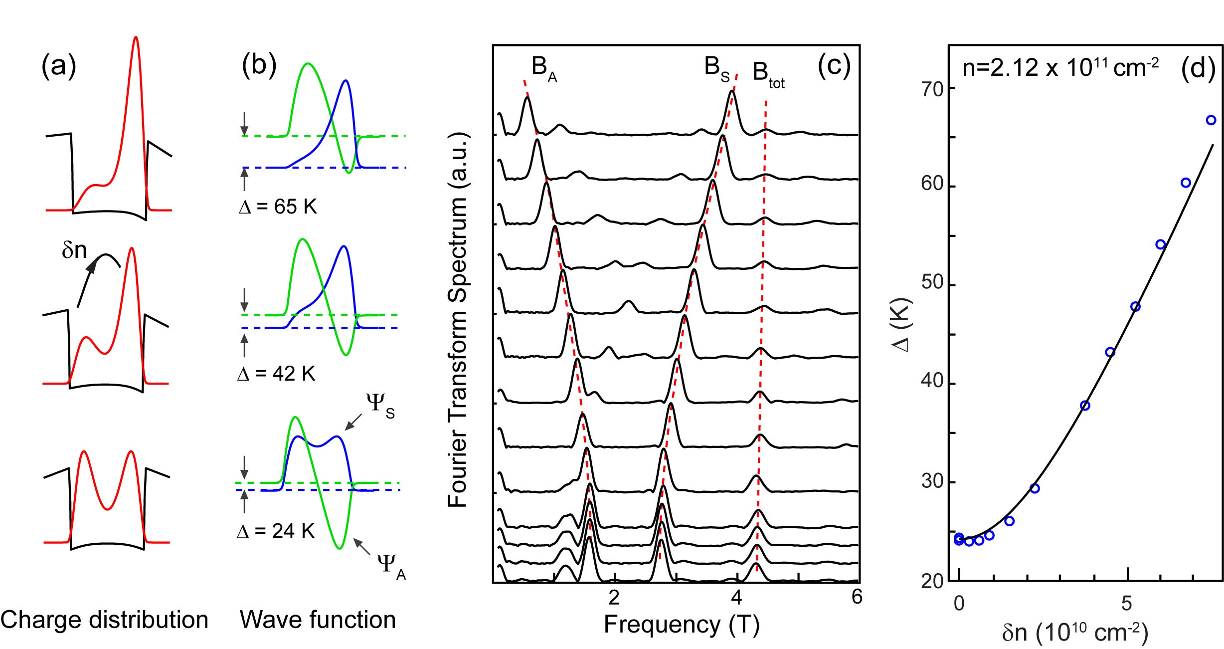
Figure 2: (a) Charge distribution (red) and potential (black), and (b) wave functions from self-consistent simulations for a 55 nm-wide GaAs QW. The charge density is kept fixed at $n=2.12\times 10^{11}$cm^-2. The subband separation $\Delta$ is the smallest when the QW is balanced (bottom panels), and increases as the QW is imbalanced. (c) The Fourier transform spectra of the measured low-field Shubnikov-de Haas oscillations. Each spectrum exhibits two main peaks, denoted as $B_{A}$ and $B_{S}$, whose separation increases as the QW is imbalanced (from bottom to top). (d) The subband separation $\Delta$ determined from the Fourier transforms through $\Delta=\frac{\hbar e}{m^{\star}}(B_{S}-B_{A})$, plotted as a function of the charge distribution asymmetry $\delta n$. The solid curve represents $\Delta$ vs. $\delta n$ from self-consistent calculations for a 55 nm-wide GaAs QW.

Our sample, grown by molecular beam epitaxy, is a 55 nm-wide GaAs quantum well (QW) bounded on each side by undoped Al_0.24Ga_0.76As spacer layers and Si $\delta$-doped layers. We fitted the sample with an evaporated Ti/Au front-gate and an In back-gate to change the 2D electron density, $n$, and tune the charge distribution symmetry and the occupancy of the two electric subbands, as demonstrated in Fig. 2. This tunability, combined with the very high mobility ($\sim$ 400 m²/Vs) of the sample, is key to our success in probing the strength of the $q/3$ states at high fillings.

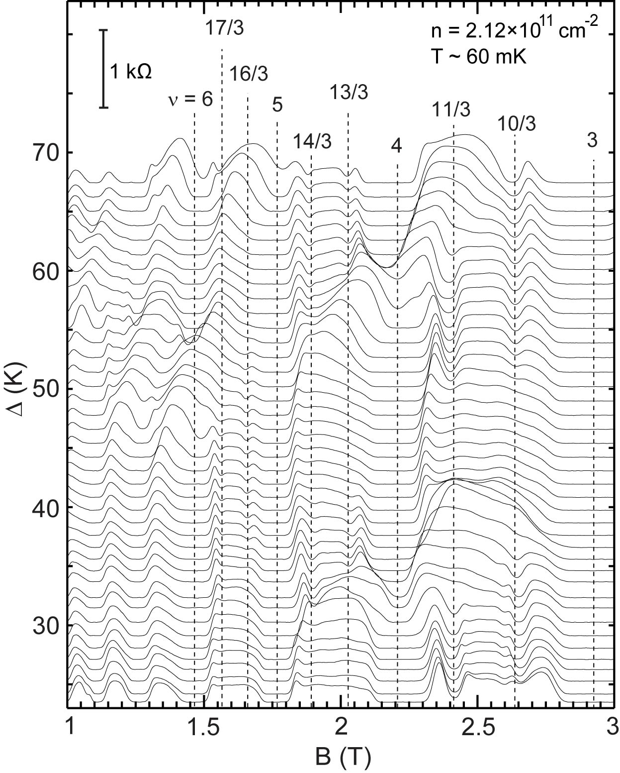
Figure 3: Waterfall plot of $R_{xx}$ vs. $B$ taken at a fixed density $n=2.12\times 10^{11}$cm^-2 as the subband separation ($\Delta$) is increased. The scale for $R_{xx}$ is indicted in the upper left (0 to 1 k$\Omega$). Each trace is shifted vertically so that its zero (of $R_{xx}$) is aligned with its measured value of $\Delta$ which is used as the y-axis of the waterfall plot. Vertical lines mark the field positions of the filling factors, $\nu$.

When the QW in our experiments is ”balanced”, i.e., the charge distribution is symmetric, the occupied subbands are the symmetric (S) and anti-symmetric (A) states (see the lower panels in Figs. 2(a) and (b)). When the QW is ”imbalanced,” the two occupied subbands are no longer symmetric or anti-symmetric; nevertheless, for brevity, we still refer to these as S (ground state) and A (excited state). In our experiments, we carefully control the electron density and charge distribution symmetry in the QW via applying back- and front-gate biases.Suen et al. (1994); Shabani et al. (2009) For each pair of gate biases, we measure the occupied subband electron densities from the Fourier transforms of the low-field ($B\leq 0.5$ T) Shubnikov-de Haas oscillations. These Fourier transforms, examples of which are shown in Fig. 2(c), exhibit two peaks ($B_{S}$ and $B_{A}$) whose frequencies, multiplied by $2e/h$, give the subband densities, $n_{S}$ and $n_{A}$. The difference between these densities directly gives the subband separation, $\Delta$, through the expression $\Delta=\frac{\pi\hbar^{2}}{m^{*}}(n_{S}-n_{A})$, where $m^{*}$ is the electron effective mass. Note that, at a fixed total density, $\Delta$ is smallest when the charge distribution is balanced and it increases as the QW is imbalanced. Figure 2(d) shows the measured $\Delta$ as a function of the charge $\delta n$ transferred between the back and front sides of the QW. Note that we measure $\delta n$ from the change in the sample density induced by the application of either the back-gate or the front-gate bias.

III magneto-transport data

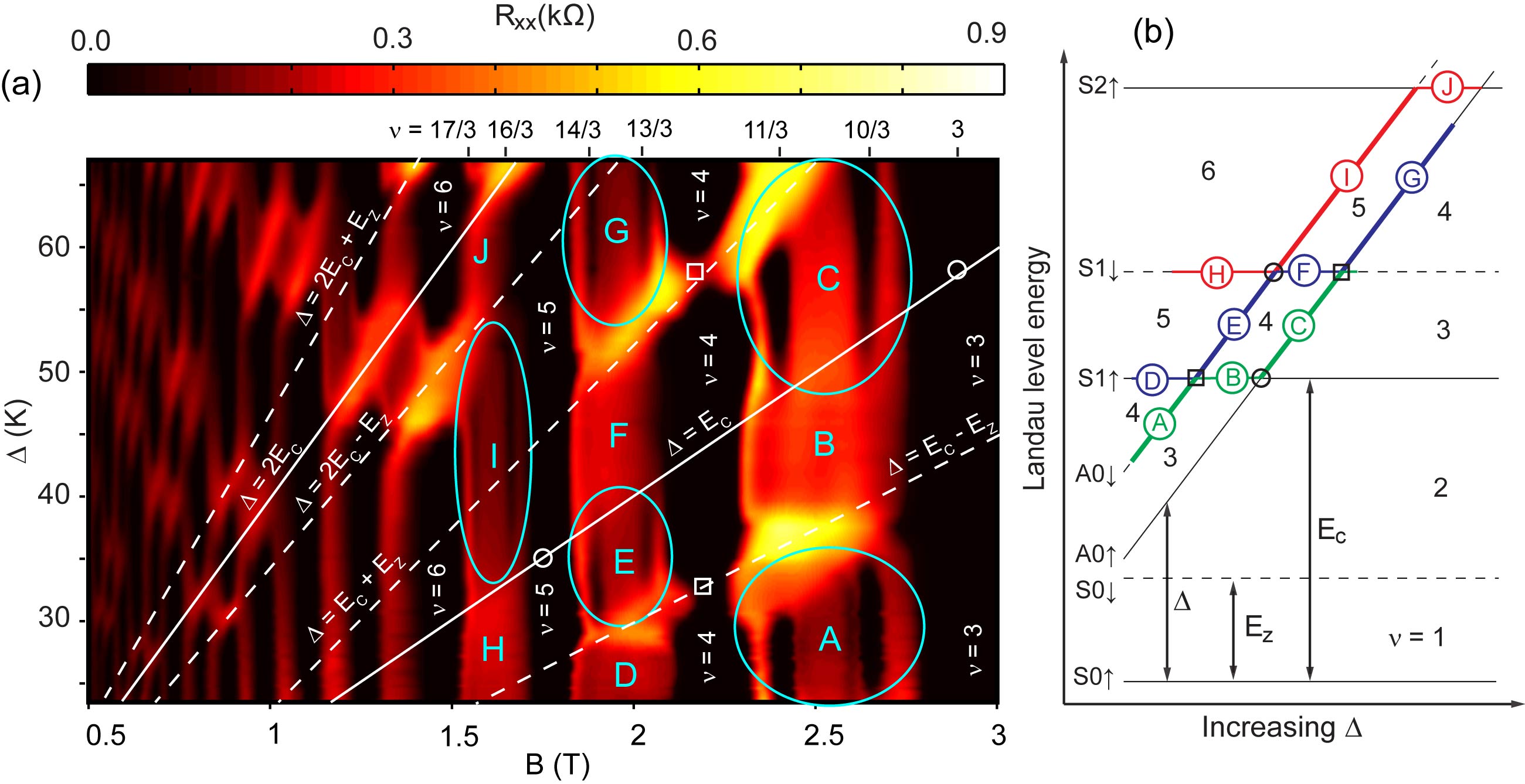
Figure 4: Evolution of $R_{xx}$ data taken at a fixed density $n=2.12\times 10^{11}$cm^-2 as the subband separation ($\Delta$) is increased. (a) A color-scale plot of the data shown in Fig. 3. The dark regions are where the integer or fractional quantum Hall states are observed at the indicated values of $\nu$. The solid white lines denote $\Delta=E_{C}$ and $\Delta=2E_{C}$, where $E_{C}$ is the cyclotron energy. The dashed white lines are drawn such that they pass through the even-filling coincidences (see text). The cyan ellipses mark different regions (A, C, E, G, and I) where FQH states are seen. (b) Schematic electron Landau level diagram as a function of increasing $\Delta$. The relevant energies, $\Delta$, the cyclotron energy ($E_{C}$), and the Zeeman energy ($E_{Z}$), are shown. The position of the Fermi level is plotted in different colors for several filling factor regions: 3 $<\nu<$ 4 (green), 4 $<\nu<$ 5 (blue), and 5 $<\nu<$ 6 (red). The letters correspond to the regions in the (a) panel; the regions where FQH states are observed are marked by thicker lines.

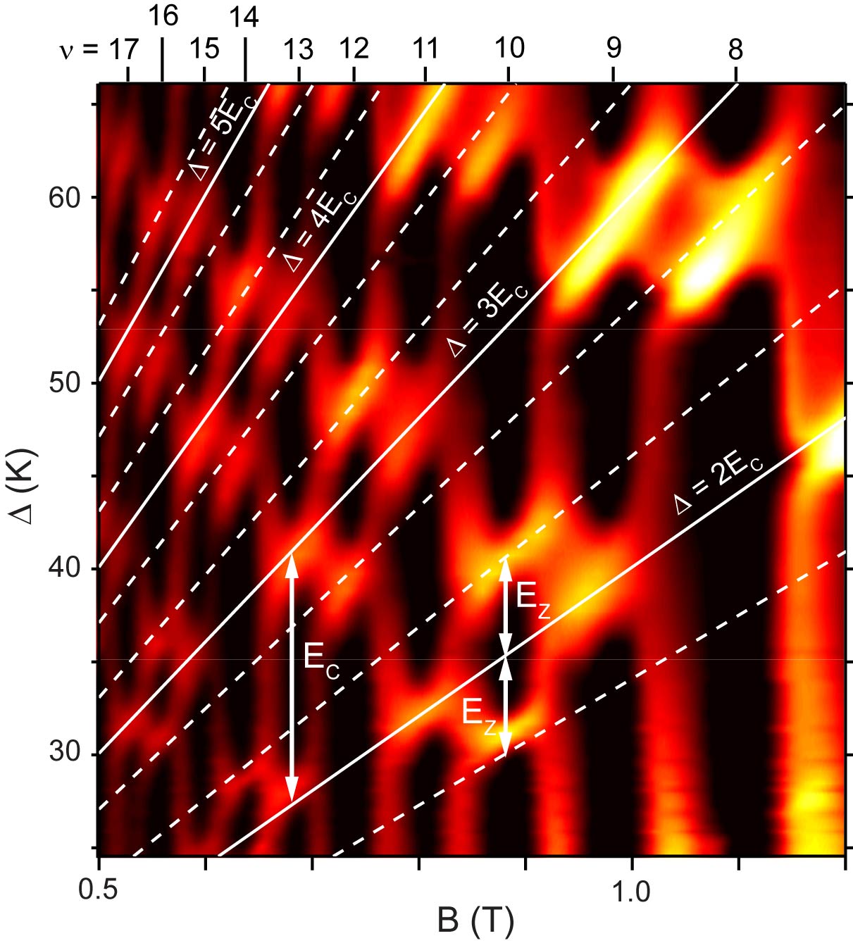
Figure 5: An expanded color-scale plot of $R_{xx}$ data at low fields for $n=2.12\times 10^{11}$ cm^-2. The solid white lines denote $\Delta=iE_{C}$ for $i=2,3,4,5$. The dashed white lines represent $\Delta=iE_{C}\pm E_{Z}$, using a fixed $g^{\star}=8.8$ (see text).

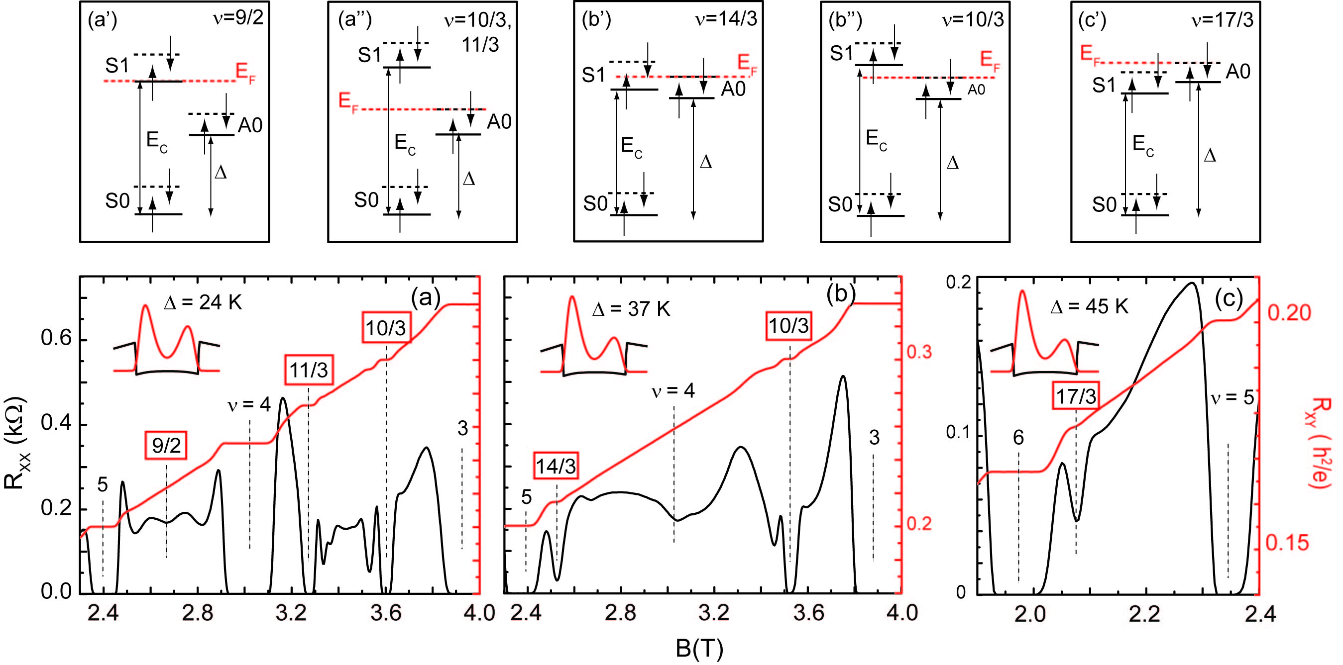
Figure 6: (a), (b), (c) Longitudinal ($R_{xx}$) and Hall ($R_{xy}$) resistances for the 55 nm-wide QW at a higher density $n=2.90\times 10^{11}$ cm^-2. Panels (a) and (b) share the same scales for $R_{xx}$ and $R_{xy}$. The traces were taken at $T=30$ mK, and the insets show the charge distributions calculated at $B=0$. The LL diagrams for fractional fillings in panels (a), (b) and (c) are shown in (a’) and (a”), (b’) and (b”), and (c’), respectively. Fractional quantum Hall states at $\nu=10/3$, 11/3, 14/3, and 17/3 are clearly seen when $E_{F}$ lies in either the A0$\uparrow$ or A0$\downarrow$ levels.

Figure 7: $R_{xx}$ and $R_{xy}$ traces at high magnetic fields and $T=30$ mK for $n=2.12\times 10^{11}$ cm^-2 for the ”balanced” QW. Fractional quantum Hall states at $\nu=4/3$, 5/3, 7/3, and 8/3 are clearly seen. The upper panels show the LL diagrams and positions of $E_{F}$ for the indicated fillings.

Figure 3 shows a series of longitudinal resistance ($R_{xx}$) vs. magnetic field ($B$) traces taken at a fixed density $n=2.12\times 10^{11}$ cm^-2 as the subband spacing is increased. The y-axis is $\Delta$, which is measured from the low-field Shubnikov-de Haas oscillations of each trace. The same data are interpolated and presented in a color-scale plot in Fig. 4(a). In Fig. 5, we show a color-scale plot of the data in the low field regime.

In Figs. 3, 4(a), and 5 we observe numerous LL coincidences at various integer filling factors, signaled by a weakening or disappearance of the $R_{xx}$ minimum. For example, the $R_{xx}$ minimum at $\nu=4$ is strong and wide at all values of $\Delta$ except near $\Delta$ = 32 and 58 K, marked by squares in Fig. 4(a), where it becomes narrow or disappears. Such coincidences can be easily explained in a simple fan diagram of the LL energies in our system as a function of increasing $\Delta$, as schematically shown in Fig. 4(b). In this figure, we denote an energy level by its subband index (S or A), LL index ($N=0,1,2,\cdots$), and spin ($\uparrow$ or $\downarrow$). Also indicated in Fig. 4(b) are the separations between various levels: the cyclotron energy ($E_{C}=\hbar eB/m^{*}$), Zeeman energy ($E_{Z}=g^{*}\mu_{B}B$, where $g^{*}$ is the effective Landé g-factor), and $\Delta$. From Fig. 4(b) it is clear that the condition for observing a LL coincidence at odd fillings is $\Delta=iE_{C}$, while for coincidences at even fillings, the condition is $\Delta=iE_{C}\pm E_{Z}$; in both cases, $i$ is a positive integer.

In Figs. 4(a) and 4(b), we have indicated the two coincidences at $\nu=4$ with squares. Note that the coincidences at even fillings correspond to a crossing of two levels with antiparallel spins. In Figs. 3 and 4(a), the coincidences at low, odd fillings (e.g., $\nu=3$ and 5) are not as easy to see at low temperatures since the resistance minima remain strong as the two LLs, which have parallel spins, cross. Such behavior has been reported previously and has been interpreted as a signature of easy-plane ferromagnetism. Jungwirth et al. (1998); Muraki et al. (2001); Vakili et al. (2006) We note that our data taken at higher temperatures ($T$ = 0.31 K) reveal a weakening of the $\nu=5$ minimum at $\Delta=35$ K, and of the $\nu=3$ minimum at $\Delta=58$ K;Shabani (2011) these are marked by circles in Fig. 4(a). The crossings at higher odd fillings are clearly seen in Figs.  4(a) and 5; e.g., the $\nu=7$ minimum disappears at around $\Delta=50$ K, and $\nu=9$ around $\Delta=$ 40 K and 60 K.

In Figs. 4(a) and 5 we include several solid white lines representing $\Delta=iE_{C}$, assuming GaAs band effective mass of $m^{*}=0.067$ (in units of free electron mass). These lines indeed pass through the positions of the $observed$ LL coincidences for odd fillings, implying that $\Delta$ is not re-normalized at LL coincidences. We note that, with the application of magnetic field, the subband electron occupation might vary because of the finite number of discrete LLs that are occupied. This could lead to a redistribution of charge which in turn could lead to changes in $\Delta$ as a function of magnetic field. At LL coincidences, however, the two crossing LLs which belong to the different subbands are energetically degenerate. If the coincidence occurs at the Fermi energy, electrons can move between the two degenerate LLs so that the subband occupancy and the charge distribution, and therefore $\Delta$, are restored back to their zero-field values. This conjecture is indeed confirmed by self-consistent calculations reported for a two-subband 2D electron system in a perpendicular magnetic field:Trott et al. (1989) While the subband occupancy and $\Delta$ oscillate with field, they equal their zero-field values whenever two LLs belonging to different subbands coincide at $E_{F}$. We conclude that the field positions of the LL coincidences at $E_{F}$ are determined by the value of $\Delta$ at $B=0$, and that the lines drawn in Figs. 4(a) and 5 accurately describe the positions of these coincidences.

The dashed lines in Figs. 4(a) and 5, represent $\Delta=iE_{C}\pm E_{Z}$, $i=1,2,...$, where $g^{*}$ is chosen as a fitting parameter so that these lines pass through the even-filling coincidences. All the dashed lines in Figs. 4(a) and 5 are drawn using $g^{*}=$ 8.8, except for the $\Delta=E_{C}\pm E_{Z}$ lines, which are drawn using $g^{*}=$ 8.9 and 7.6, respectively. We conclude that $g^{*}$ is enhanced by a factor of $\sim$ 20 relative to the GaAs band g-factor (0.44). This enhancement is somewhat larger than the values reported for GaAs QWs with two subbands occupied. For example, Muraki $et\ al.$ Muraki et al. (2001) reported a $\sim$ 10-fold enhancement of $g^{*}$ for electrons in a 40 nm-wide QW with $n\sim 3\times 10^{11}$ cm^-2 while Zhang $et\ al.$ Zhang et al. (2006) measured a $\sim$ 5-fold enhancement in a 24 nm-wide QW with $n\sim 7\times 10^{11}$ cm^-2. It appears then that the enhancement depends on the QW width and electron density, and a systematic study of the enhancement would be an interesting future project. However, we would like to emphasize that the dashed lines in Figs. 4(a) and 5 pass through nearly all of the observed coincidences quite well. Since each of these lines are drown using very similar $g^{*}$, the data imply that the enhancement is nearly independent of the filling factor.

We now focus on the main finding of our work, namely the correspondence between the stability of the FQH states and the position of $E_{F}$. Note in Figs. 3 and 4(a) that FQH states are observed only in certain ranges of $\Delta$. For example, the $\nu=10/3$ and 11/3 states are seen in the regions marked by A and C in Fig. 4(a) but they are essentially absent in the B region. The $\nu=13/3$ and 14/3 states, on the other hand, are absent in regions D and F while they are clearly seen in regions E and G.

To understand this behavior, in the fan diagram of Fig. 4(b) we have highlighted the position of $E_{F}$ as a function of $\Delta$ for different filling factors by color-coded lines. Concentrating on the range $3<\nu<4$ (green line in Fig. 4(b)), at small values of $\Delta$ (region A), $E_{F}$ lies in the A0$\downarrow$ level. At higher $\Delta$, past the first $\nu=4$ coincidence which occurs when $\Delta=E_{C}-E_{Z}$, $E_{F}$ is in the S1$\uparrow$ level (region B). Once $\Delta$ exceeds $E_{C}$, $E_{F}$ lies in the A0$\uparrow$ level (region C) until the second $\nu=4$ coincidence occurs when $\Delta=E_{C}+E_{Z}$. Note in Fig. 4(a) that strong FQH states at $\nu=10/3$ and $11/3$ are seen in regions A and C. From the fan diagram of Fig. 4(b) it is clear that in these regions $E_{F}$ is in the $ground$-$state$ ($N=0$) LLs of the asymmetric subband, i.e., A0$\uparrow$ and A0$\downarrow$. In contrast, in region B, where the 10/3 and 11/3 states are essentially absent, $E_{F}$ lies in an $excited$ ($N=1$) LL, namely, S1$\uparrow$. We conclude that the 10/3 and 11/3 FQH states are stable and strong when $E_{F}$ lies in a ground-state LL.

The data in the range $4<\nu<5$ corroborate the above conclusion. In Fig. 4(b) we represent the position of $E_{F}$ in this filling range by a blue line. In regions E and G, $E_{F}$ lies in the ground-state LLs of the asymmetric subband (A0$\downarrow$ and A0$\uparrow$), and these regions are indeed where the $\nu=13/3$ and 14/3 FQH states are seen. In regions D and F, on the other hand, $E_{F}$ is in the excited LLs of the symmetric subband (S1$\uparrow$ and S1$\downarrow$), and the 13/3 and 14/3 FQH states are absent. Data at yet higher fillings ($5<\nu<6$) follow the same trend: FQH states at $\nu=16/3$ and 17/3 are seen in region I when $E_{F}$ is in the A0$\downarrow$ level, but they are absent in regions H or J where $E_{F}$ lies in the S1$\downarrow$ or S2$\uparrow$ levels.

In Fig. 6 we show additional data for a density of $n=2.90\times 10^{11}$ cm^-2 in the same QW. Longitudinal and Hall resistance traces are shown in the bottom panels for three different values of $\Delta$, and in each panel the calculated charge distribution (at $B=0$) is also shown. In the top panels, we show the positions of the LLs and $E_{F}$, corresponding to the filling factors in the bottom panels. In all cases, strong $q/3$ FQH states are observed when $E_{F}$ lies in the $N=0$ of the A0$\downarrow$ level. Note that the data shown in Fig. 6 are for asymmetric charge distributions. We would like to emphasize that strong $q/3$ states are also observed for symmetric (”balanced”) charge distributions; e.g., see the bottom trace in Fig. 3, or the traces in Fig. 2(c) of Shabani $et$ $al.$ Shabani et al. (2010)

Next we address the FQH states observed at lower $\nu$ ($<3$) in our sample. Data are shown for $n=2.12\times 10^{11}$ cm^-2 for the ”balanced” QW ($\Delta=23$ K) in Fig. 7; the $R_{xx}$ trace is an extension of the lowest trace shown in Fig. 3. In the range 1 $<\nu<$ 3, strong FQH states are seen at $\nu=$ 4/3, 5/3, 7/3 and 8/3. Data taken at yet higher magnetic fields (not shown) reveal the presence of a very strong FQH state at $\nu$ = 2/3. From the fan diagram of Fig. 4(b), it is clear that $E_{F}$ at these fillings lies in an $N=0$ LL, namely, the A0$\uparrow$ ($\nu=$ 7/3 and 8/3), S0$\downarrow$ ($\nu=$ 4/3 and 5/3), or S0$\uparrow$ ($\nu=$ 2/3) levels.

IV discussion

Our observations provide direct evidence that the $q/3$ FQH states are strong when $E_{F}$ resides in a ground-state ($N=0$) LL, regardless of whether that LL belongs to the A or S subband. This finding implies that the node in the wavefunction in the $out$-$of$-$plane$ direction does not significantly de-stabilize the $q/3$ FQH states. On the other hand, when $E_{F}$ lies in an $N>0$ LL, the wavefunction node(s) in the $in$-$plane$ direction weaken or completely de-stabilize the $q/3$ FQH states. These conclusions are consistent with the data from single-subband samples, Pan et al. (1999); Lilly et al. (1999); Du et al. (1999); Gervais et al. (2004) as well as theoretical calculations. Haldane (1987); MacDonald and Girvin (1986); d’Ambrumenil and Reynolds (1988); Koulakov et al. (1996); Moessner and Chalker (1996); Töke et al. (2005) In a composite Fermion picture, our data also imply that the lower lying (fully occupied) LLs are essentially inert and the composite Fermions are formed in the partially filled LL where $E_{F}$ lies. The composite Fermions, however, could have a spin and/or subband degree of freedom, as we briefly discuss in the last paragraph of this section (see also, Ref. Shabani et al., 2010).

Our data also allow us to assess the stability of the FQH states as two LLs approach each other. In Fig. 4(a) the dashed line denoted $E_{C}-E_{Z}$ marks the position of the expected crossing between the A0$\downarrow$ and the S1$\uparrow$ levels, based on the LL coincidence we observe for the $\nu=4$ quantum Hall state. It is clear in Fig. 4(a) that as we approach this line from the A region, the 10/3 and 11/3 FQH states disappear when $\Delta$ is about 5 K away from $E_{C}-E_{Z}$. A similar statement can be made regarding the stability of the 11/3 state as the $E_{C}+E_{Z}$ dashed line is approached from the C region, and the stability of the 13/3 and 14/3 states as one approaches the $E_{C}+E_{Z}$ line from the G region or the $E_{C}-E_{Z}$ line from the E region.Note (4) Note that what is common to all these observations is that the boundaries marked by the dashed lines correspond to the crossing of two LLs with $antiparallel$ spins.

Data of Fig. 4(a) suggest that, when the two approaching LLs have $parallel$ spins, the $q/3$ states remain stable even closer to the expected LL crossings. For example, the 10/3 and 11/3 FQH states in region C are stable very close to the boundary (the line marked $E_{C}$) separating this region from B. Similarly, the 13/3 and 14/3 states are stable in region E close to the $E_{C}$ line separating E from F. Note that in both cases, i.e., traversing from C to B or from E to F, the two approaching LLs have parallel spins (see Fig. 4(b)). We conclude that the relative spins of the two approaching LLs also play a role in the stability of the $q/3$ FQH states. It is worth emphasizing that, as is evident from Figs. 3 and 4(a) data, the relative spins of the two approaching LLs also play a crucial role in the stability of the $integer$ quantum Hall (IQH) states. For antiparallel-spin LLs, the IQH state (e.g., at $\nu=4$) becomes very weak or completely disappears, while for the parallel-spin LLs the IQH state (e.g., at $\nu=3$), remains strong. This behavior has been attributed to easy-axis (for an opposite-spin crossing) and easy-plane (for a same-spin crossing) ferromagnetism. Muraki et al. (2001); Vakili et al. (2006); Jungwirth et al. (1998)

We highlight three further observations. First, strong FQH states at large $q/3$ fillings have been recently observed in very high quality graphene samples.Dean et al. (2010) These states qualitatively resemble what we see in our two-subband system. It is tempting to associate the valley degree of freedom in graphene with the subband degree of freedom in our sample. But the LL structure in graphene is of course different from GaAs so it is not obvious if this association is valid. Second, data taken in the $N$ = 1 LL at very low temperatures and in the highest quality, single-subband samples exhibit FQH states at even-denominator fillings $\nu$ = 5/2 and 7/2. Willett et al. (1987); Pan et al. (2008) In the traces shown in Fig. 3, we do not see any even-denominator states when $N$ = 1, e.g., at $\nu$ = 7/2 in region B where $E_{F}$ is in the S1$\uparrow$ level. However, in the same sample, at higher densities ($n>3.4\times 10^{11}$ cm^-2) and at low temperatures ($T=$ 30 mK), we do indeed observe a FQH state at $\nu$ = 7/2 flanked by very weak 10/3 and 11/3 states when $E_{F}$ lies in the S1$\uparrow$ level. Shabani et al. (2010)

Third, in the $N=0$ LL, high-quality samples show strong higher-order, odd-denominator FQH states at composite Fermion filling factor sequences such as 2/5, 3/7, 4/9, etc.Jain (2007) We do observe a qualitatively similar behavior in our data when $E_{F}$ is in an $N$ = 0 LL. For example, in region A (Figs. 3 and 4(a)) we see weak but clear minima at $\nu$ = 17/5 next to the 10/3 minimum. Again, at higher densities and low temperatures, such states become more developed. Shabani et al. (2010) In Fig. 1(b), for example, there are strong minima at $\nu=$ 12/5 and 13/5, adjacent to the 7/3 and 8/3 minima, and at 17/5 and 18/5, adjacent to the 10/3 and 11/3 minima. These states, as well as the $q/3$ states, exhibit subtle evolutions even when $E_{F}$ lies within a fixed $N=0$ LL, consistent with the presence of composite Fermions which have spin and/or subband degrees of freedom.Shabani et al. (2010) A related question concerns the role of charge distribution symmetry in the stability of the $q/3$ states. In other words, in a QW with fixed width, density and filling, and with $E_{F}$ in a particular $N=0$ LL, how does the strength of given a FQH state at a particular filling vary with charge distribution symmetry. We do not have data to answer this question quantitatively, but the data we present here clearly indicates that a primary factor determining the strength of the $q/3$ FQH states is whether or not $E_{F}$ lies in an $N=0$ LL.

V summary

In conclusion, the position of $E_{F}$ is what determines the stability of odd-denominator, $q/3$ FQH states at a given filling factor. When $E_{F}$ lies in a ground-state ($N=0$) LL, the $q/3$ FQH states are stable and strong, regardless of whether that LL belongs to the symmetric or antisymmetric subband. This observation implies that the wavefunction node in the out-of-plane direction is not detrimental to the stability of these FQH states. Also, the $q/3$ FQH states appear to be stable very near the crossing of two LLs, especially if the LLs have parallel spins.