Open issues in probing interiors of solar-like oscillating main sequence stars
1. From the Sun to nearly suns

Abstract

We review some major, open issues in the current modelling of low and intermediate mass, main sequence stars based on seismological studies. In the present paper, the solar case is discussed together with current problems that are common to the Sun and stars with a structure similar to that of the Sun. Several additional issues specific to main sequence stars other than the Sun are reviewed and illustrated with a few stars observed with CoRoT in a companion paper.

1 Introduction

After more than two decades of helioseismology, almost four years of asteroseismology with CoRoT [1] and almost two years of intensive asteroseismology with Kepler [2], we review some major, current open issues about the internal structure of the Sun and solar-like oscillating stars. We discuss here the solar case, this also applies to oscillating stars that have a similar internal structure. For sake of brevity, we decided to include only unpublished figures and to cite published figures in the text. Several recent reviews exist on the topic, for instance [3], [4], [5].

2 The Sun

As it is well known, the Sun is a particular case. It is the closest star, and as a result we know with a high precision the luminosity, mass (through the product $GM_{\odot}$), radius, age and individual surface abundances of chemical elements. Furthermore, a wealth of very accurate seismic constraints are available and have been successfully used. Inversion of a large set of mode frequencies has provided crucial information on the structure of the Sun, see for instance [5]; [6]. Accordingly, the following constraints must all be satisfied by any calibrated solar model: radius at the base of the convective envelope $r_{bzc}$, surface helium abundance $Y_{s}$, sound speed profile $c(r)$, internal rotation profile and location of ionization regions. To some extent, these constraints are found to be independent of the reference model [7]. The current major challenges and open issues in the solar case then are:

• what are the values of the surface abundances, more specifically the oxygen abundance?

• what is the origin of the discrepancy between the seismic sound speed and that given by models below the convection zone?

• what are the dominant physical mechanisms responsible for a uniform rotation in the radiative region and a differential rotation in the convective zone? It is worth noting that this is the opposite in current calibrated 1D solar models: the convection zone is assumed to rotate uniformly and the rotation profile in the radiative zone is found to vary with radius if waves and/or magnetic field are not taken into account (see below) !

• how can we model properly near surface layers and the convection-pulsation interaction?

• how to succeed in probing the core?

• how to model oscillation mode line widths and amplitudes?

Some of these uncertainties about the Sun have consequences on the modelling of stars other than the Sun. On the other hand, some problems that are encountered with seismological studies of stars other than the Sun can be studied first with our well known Sun. These two points of view are discussed below.

2.1 Initial abundances: the solar mixture

In the late nineties, with the GN93 solar abundances [8], the seismic sun and calibrated solar models were in agreement by 1 to 5% for the sound speed profile and location of the base of the convective zone [9]. However between 1993 and 2010 several revisions of the photospheric solar mixture were performed. Noteworthy, 3D model atmospheres including NLTE effects and improved atomic data have led to a substantial decrease of the C, N, O, Ne, Ar abundances and in turn to an important decrease of the solar metallicity $(Z/X)$ (see Table 1).

Table 1: Value of the solar photospheric metallicity from 1993 to 2010 from Table 4 in Asplund et al. [10] complemented by Caffau et al. [11]

	GN93	GS98	AGS05	AGS09	Lod09	Caff10
$Z/X$	0.0244	0.0231	0.0165	0.0181	0.0191	0.0209

Today, an internal consistency of the abundance determination from different ionization levels of a given element seems to have been obtained and a consensus between independent determinations seems to be reached (i.e. this shows the unvaluable benefit of independent approaches). However the revised modern solar chemical composition [10] leads to a strong disagreement between the sound speed of a calibrated solar model and that of the seismic Sun. This is also true for the depth of the convection zone and the envelope helium abundance (see [5], for a review). Fig.1 shows the difference of the sound speed profile between Basu’s seismic model [12] and several models computed with Cesam2k [13] using some of the abundance mixtures listed in Tab.1. This figure shows that the discrepancy at the base of the convection zone is strongly increased when the revised abundance mixture AGS05 is used. This is mainly due to the decrease in oxygen and neon and in $(Z/X)_{s}$ which consequence is a decrease of the radiative opacities. With the newly derived abundance mixture AGS09 which has achieved some consensus, the discrepancy slightly decreases but remains significant.

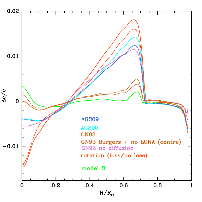
Figure 1: Differences in the sound speed profiles for the Sun between Basu’s seismic model and calibrated solar models using various abundance mixtures and different assumptions for the physical description. All models have been calculated with the Cesam2k code except model S [14] which is based on the old solar mixture.

2.1.1 Possible origins of the discrepancy

First there could be some errors in the opacity derivation. As a check, the comparison between OPAL and OP opacities for a calibrated solar model shows that OP opacities give a (slightly) better fit than OPAL. However a change in opacity of about 30% at the base of the convection zone, at a temperature of $2~{}10^{6}$ K would be necessary to compensate for the effects of the change in mixture [15, 3] and according to [16] there appears to be no way to change the OP opacity by such an amount (see also [17] and [18]). Other possible causes have been discussed but none of the related improvements can reconcile simultaneously all the seismic constraints listed above [19],[20], [21].

In order to reconcile the seismic and theoretical sound speed, one needs higher opacities or higher helium below the upper convective zone (UZC) i.e. a higher He gradient. Any mixing below the UZC which smooths the gradient therefore would go in the wrong direction. In that case, one would rather need an advection process. It is not clear whether internal waves and/or which hydrodynamical instability could act in the sense of increasing helium below the UZC. Other further developements are underway such as taking magnetic effects into account in the derivation of solar abundance corrections. An investigation based on 3D magnetoconvection simulations shows that corrections to the solar abundance can be significant [22].

Abundances of other stars are determined by reference to the Sun, hence all stars are affected by errors or by inaccuracies in the solar mixture. Can other stars be discriminating in that issue? Note that one must wonder about the impact of the inconsistency which arises when modeling other stars using solar mixtures inferred from 3D model atmospheres if the stellar [Fe/H] itself has not been determined from a dedicated 3D model atmosphere.

2.2 Nuclear reaction rates

In stars, (most commonly charged induced) nuclear reactions occur at low energies (10- 300 keV) in the Gamow peak -which corresponds to the maximum probability of the reaction. The cross sections that are governed by Coulomb barriers and resonances show a strong and complex dependance on energy and globally decrease steeply towards low energy.

Cross sections are usually written in the form

$$\sigma(E)={S(E)\over E}~{}e^{-2\pi\eta}$$ (1)

where $S(E)$ -the astrophysical factor- contains everything that concerns the nuclei and nuclear physics and varies slowly with $E$. The exponential term is related to the Coulomb barrier and relative velocity of the nuclei. Experiments which provide measurements of the cross sections in the laboratory generally occur at higher energy than the Gamow peak. Extrapolation of $S(E)$ to lower $E$ is then necessary. This is difficult to achieve and cannot take into account possible unknown resonances occuring at low $E$. When the $S$-factor cannot be measured, the reaction rates are obtained from pure theory. Recent significant progress in laboratory and theory (hence better determination of $S$-factors down to the Gamow peak) has been achieved as discussed in the comprehensive reviews by [23], [24], see also [25].

2.2.1 Hydrogen burning reaction rates:

Uncertainties still exist for the pp chain and CNO cycle reaction cross sections in the Sun. They are due to the difficulty to estimate the $S$-factor at low energy and to determine the exact role of the electron screening (both in the laboratory and in the star). For most of the concerned reactions, $S$-factors are determined from extrapolation of experimental data to low $E$ but now, for some key reactions, energies corresponding to the Gamow peak are accessible through measurements provided by the LUNA experiment at Gran Sasso [26]. This is the case of the ${}^{3}He(^{3}He,2p)^{4}He$ reaction (see Fig. 1 in [26]) for which the $S(E)$-value has not been significantly modified but the error bars are largely decreased. Furthermore the cross section of the $N^{14}(p,\gamma)O^{15}$ reaction -the leading reaction in the CNO cycle- has now been measured down to energies relevant for $1M_{\odot}$ stars on the red giant branch (see Fig. 19 in [26]) and a resonance is observed. This represents a significant advance although an extrapolation is still needed towards solar conditions. Noteworthy, the revision is important with a decrease of $S(E)$ by 50%. This has crucial consequences for solar and stellar structure. In the solar core, the CNO cycle efficiency is reduced from $1.6$ to $0.8\%$ of the total energy. For main sequence stars slightly more massive than the Sun the occurrence of a convective core depends on the energy production. With the new $N^{14}(p,\gamma)O^{15}$ rate the convective core appears at higher stellar mass and is less massive for a given mass (see for instance the case of a 1.2 $M_{\odot}$ low metallicity star in Fig. 14 by [27]). Finally cross sections that are obtained from pure theory can be constrained by helioseismology [28],[29],[23].

2.2.2 Electron Screening

Electron screening is based on the Salpeter’s formula [30] with the underlying physical picture: the cloud of electrons decrease the repulsive Coulomb effect between interacting nuclei with the result of a decrease of the Coulomb potential and an enhancement of the reaction rate. This is a static description. It is currently not clear whether dynamic effects of the interacting ions can significantly change the impact of the screening in nuclear interactions for stars and wherther it must therefore be taken into account. The energy that initially fast moving interacting ions have when they get close enough to interact can be lower than the mean value of the medium; accordingly their reaction rate is reduced compared to Salpeter’s prescription. This effect is difficult to quantify and relies on results from numerical simulations [31], [32], [33], [34] and the issue is not settled yet. [29] looked at the impact of changing the electron screening compared with the classical Salpeter’s formula on the solar sound speed profile. They found that the solar seismic constraints do not allow variations larger than 1% when using GS98. [3] computed a solar model equivalent to the S model but assuming the extreme case of no screening at all. Their Fig.12 shows the difference in the sound speed profile between the seismic sun [12] and model S but switching off e- screening. A decrease of the reaction rate by swithcing off the e-screening clearly increases the discrepancy between observation and model. This is in agreement with previous results of [23] who showed that the large sound speed discrepancy with the use of AGS05 mixture is reduced to the previous level obtained with GS98 when the pp-reaction and the screening factor are increased up to 15% (Fig.3 in [23]) In that case, the surface helium and the depth of the convective envelope are in agreement with seismic determinations but the sound speed profile in the core significantly deviates from the seismic solar sound speed.

2.3 Transport of chemicals and angular momentum

Rotationally induced transport The physical origin of the uniform rotation profile in the radiative zone of the Sun unravelled by helioseismology is still debated. Rotationally induced transport of angular momentum resulting from a competition between shear-induced turbulence and meridional circulation driven by surface angular momentum losses is not able to make the rotation uniform in the radiative region of the Sun. For details, the reader is refered to [35]. The impact of rotationally induced transport on the solar sound speed profile has been investigated by [36]; [37]. [38] have computed a solar model including rotationally induced transport with two different assumptions about the initial velocity (slow or ‘fast’ sun). Their conclusion is that for an initially slow rotation, the microscopic diffusion dominates whereas for an initially rapid enough rotation, meridional circulation dominates over turbulent shear. However in both cases, the discrepancy below the UCZ increases (see Fig.9 of [38]). This is also illustrated in Fig.1 which shows the differences in sound speed profile for calibrated solar models computed with AGS05 mixture computed assuming either no rotationally induced transport, or rotationally induced transport with no surface angular momentum loss or assuming rotationally induced transport with surface angular momentum loss. Adding rotationally induced transport makes the discrepancy with the observed sound speed worse. Indeed this process smoothes the helium gradient below the UZC whereas the observations seem to require an increase of helium in the radiative zone below the UCZ. Several prescriptions have been derived for the turbulent transport coefficients involved in rotationally induced transport but validitation of these prescriptions remain to be done [39].
Internal wave induced transport in radiative zones must exist in stars as these waves are generated at the interface between convective and radiative regions. They have been shown to transport angular momentum efficiently enough to make the rotation of the Sun in its radiative part rigid [40]. One the main uncertainties is related to the absence of a viable quantitative description of the generation of waves.
Magnetic induced transport Instabilities driven by the interaction between rotation and a magnetic field could be responsible for the transport of angular momentum and the rigid solar rotation [41]. This was shown by [37] in the solar case.

Whether all 3 processes work together to shape the solar rotation profile in the radiative zone or only one or two are dominant is not settled yet.

Investigations of the impact of rotationally and wave induced transport on the structure of stars other than the Sun have been performed for instance to explain the Li dip [42]; [43]. [44] studied the impact of including both rotationally induced transport and magnetic field on the structure of solar like stars while [45] estimate the seismic consequences and find that with the type of dynamo they assume in the radiative zone, the efficiency of rotational mixing in a radiative zone is significantly decreased and seismic parameters are then similar to those of a non-rotating, non-magnetic star.

2.4 Near surface layers

A direct comparison of the observed and numerical frequencies of the Sun shows systematic differences that remain small at low frequency but increase with increasing frequency [46]. Several causes contribute to this offset with more or less importance [47]. They are collectively referred to as near-surface effects (for reviews, see for instance [48], [4]).

2.4.1 Surface turbulent convection

One important contribution to the differences between the observed and calculated frequencies comes from current modelling of the outer turbulent convective layers of the Sun. The description of the convective outer layers of the Sun in 1D stellar models remains quite approximate due to our inability to represent and implement in a 1D code a 3D multiscale nonlocal process such as turbulent dynamics [49]. At the solar surface, turbulent convection is inefficient and therefore strongly dependent on the free parameters entering the local, 1D formulation for convection as well as many other assumptions in the formulation. A comparison between frequencies computed with two of the available formulations (MLT and CM [50]) for instance shows that the frequency differences increase with frequency and reach up to $0.15\%$ at a frequency $\nu=4.$ mHz i.e. a frequency offset of about $6-10\mu$Hz ([9]).
Patched models, that is 1D stellar models where the outer layers have been replaced in a proper way by those obtained with 3D numerical simulations, lead to frequencies in much better agreement with the observations [51], [52], [53], [54]. For reviews, see [55], [56]. This approach is valuable for studies of individual stars provided great care is taken in the patching procedure, but it cannot be used in a systematic investigation of a large number of stars. Indeed 3D numerical simulations with the required quality are quite numerical time consuming and therefore not available in the whole range of effective temperature, gravity and chemical composition.

Atmosphere as boundary condition:

Another longstanding problem is the description of the atmosphere as boundary condition when computing a stellar model [57]. In the solar case, one can use an empirical atmosphere derived from observations (HSRA) [58] which represents accurately enough the Sun atmospheric properties. But in other stars, one must rely on atmospheres built using a temperature-optical depth, $T(\tau)$, law. Commonly used $T(\tau)$ laws are the Eddington law or more realistic Kurucz model atmospheres [59]. In order to illustrate the impact of the atmosphere boundary condition, Fig.2 (left panel) shows an echelle diagram built from observed solar oscillation frequencies based on SOHO data. An echelle diagram computed for a calibrated solar model where the temperature stratification of the atmosphere is assumed to follow a Eddington $T(\tau)$ law is also shown (middle panel). Largest differences are seen at high frequency. They are significantly larger than the observational errors. The discrepancy at high frequency decreases (roughly by half) when a more realistic Kurucz model is used (middle panel) . However one needs extensive grids of such models along an evolutionary track and for different masses. Furthermore, model atmospheres suffer from physical imperfections and are not applicable over the entire range of needed masses and ages (i.e. gravity, effective temperature) [60].

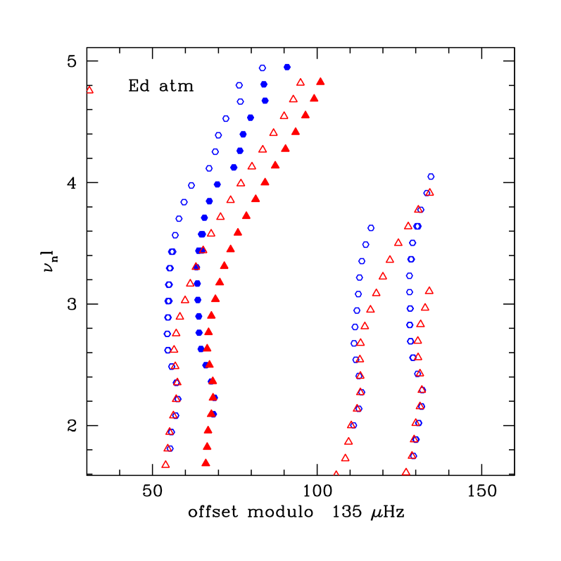
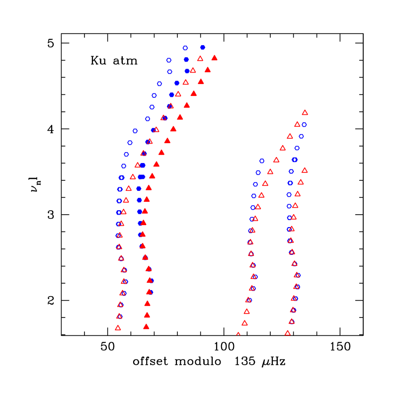
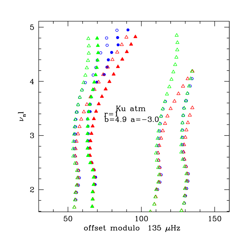
Figure 2: Echelle diagrams computed with GOLF solar data (blue dots) and using a calibrated solar model computed with either an Eddington (left panel) or a Kurucz (middle panel) $T(\tau)$ law (red dots) . Filled symbols correspond to radial modes. Right panel: An additional echelle diagram obtained from frequencies of the solar model (red dots) but corrected for near surface effects (green dots) agrees with the observations (blue dots) over the fitted interval.

Nonadiabatic effects:

Another source of uncertainty comes from what is usually referred to as nonadiabatic effects. They include the effects of interaction of the wave with the radiation and with the convection (see for instance [48]).

All these imperfections concur to generate significant errors on the computed oscillation frequencies which in the solar case amount up to 10 $\mu$Hz at high frequency. As near surface effects cannot yet be reliably included in theoretical frequency computations, an alternative has been proposed which consists in removing these effects from observed frequencies. In the solar case, this has been quantitatively assessed with the comparison of theoretical and observed frequencies of modes with small to large degrees.

2.4.2 Correcting frequencies for near surface effects

In the solar case, due to the large number of different modes, near surface effects can be removed from the frequencies. However, other procedures must be found for stars other than the Sun. Several approaches have been proposed. One consists in comparing the ratio of frequency combinations rather than frequencies themselves for low degree modes. In that case indeed near surface effects are at least partially cancelled [61]. On the other hand, in order to be able to use absolute frequencies, [62] proposed a means to correct observed frequencies for near surface effects. They first showed that the systematic offset between the observed and theoretically computed frequencies of the Sun is well fitted with a power law

$$\nu_{mod}(n)=\nu_{obs}(n)-a(\nu_{obs}(n)/\nu_{max})^{b}$$ (2)

with $a,b$ fit to the data and $\nu_{max}=3100$ Hz is a reference frequency that corresponds to the frequency of maximum power in a power spectrum. The frequencies $\nu_{obs}(n)$ and $\nu_{mod}(n)$ respectively represent the observed and model frequencies of radial modes with radial order $n$. For the Sun, such a correction leads for instance to small separations $d_{02}$ which yield a solar age consistent with the meteoritic age [63].

Fig.2 (right panel) illustrates the effect of correcting $l=0$ frequencies from near surface effects according to Eq.2 with $r=1,a=-3.0,b=4.9$ for the same solar model (with Kurucz $T(\tau)$ law) as in the middle panel. The corrected frequency echelle diagram coincides with the observations over the frequency interval that was used to derive the parameter values $a,b$. The next question is: how much the parameters a,b, $\nu_{0}$ do depend on the adopted (Kurucz or another) model atmosphere? Of course one must also keep in mind that the values of the fitted parameters are valid only over the fitted observed frequency domain (see Fig.2 left).

Whether the above procedure can be applied to stars that are different from the Sun is an open question. Elements of the answer can be obtained with the use of available 3D numerical simulations and 1D patched models. Frequency differences for radial modes between a solar patched model and a non patched model are displayed in Fig.3 (left) as a function of the radial mode frequency of the patched model scaled to the frequency $\nu_{max,\odot}$ given according to [64] scaling law. The curve $a(\nu_{patch}/\nu_{max})^{b}$ is also plotted and coincides with the observations over the frequency interval that was used to derive the $a,b$ parameter values over an interval up to $\nu_{patch}/\nu_{max}\approx 1.2$. Similar plots are displayed in Fig.3 (right) for 3 other models with different effective temperature, gravity or chemical abundance. For these models, we take again $\nu_{max}$ according to [64] and $T_{eff,\odot}$ and $\nu_{max,\odot}$ from our solar patched model. The parameters $a,b$ are adapted to fit the frequency differences over the largest $\nu_{patch}/\nu_{max}$ interval. Again a power law can fit the frequency differences over an interval up to $\nu_{patch}/\nu_{max}\approx 1.2-1.4$. We note that the frequency differences for the 3 models behave differently at high frequency than the solar ones. This is likely due to their lower gravity, higher effective temperature. Indeed, for these models, the ratio of turbulent to total pressure is higher than for the solar model (the higher the effective temperature, the lower the gravity, the higher the ratio $P_{turb}/P_{tot}$) and this results in larger differences between patched and non patched models. Note that for the three models (all three hotter than the solar model), the frequency differences show an oscillating behavior in function of the scaled frequency. Whether this behavior is real or artificially introduced by the patching process is not known yet. In any case, at lower frequency, the mean variation with frequency is well reproduced by a power law up to $\nu_{patch}/\nu_{max}\approx 1.2-1.4$

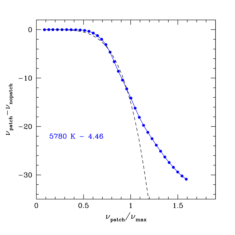
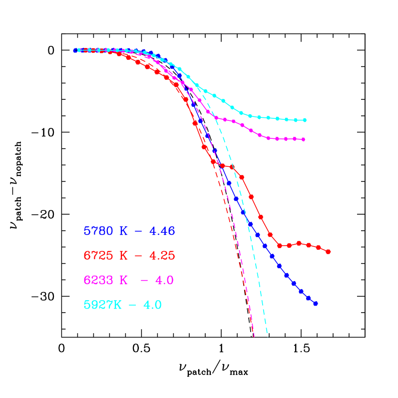
Figure 3: left: Frequency differences for radial modes $\nu_{patch}-\nu_{nopatch}$ between a patched and a non patched solar models (blue dots) as a function of $\nu_{patch}/\nu_{max}$. The black dashed line represents the power law according to Eq. 2 with $\nu_{max}=3.207$mHz,$r=1,a=-15,b=4.9$ (For the solar models: $T_{eff}=5780,g=4.46$). right: Same as left for stellar models with different effective temperature, gravity as labelled in the left corner. Magenta and red models have a solar metallicity whereas the cyan models have a lower metallicity $[Fe/H]=-1$. Coloured dashed lines represent the power law according to Eq. 2 for each corresponding frequency difference. Parameter values are $\nu_{max}=1.462$mHz, $r=1,a=-17,b=3.9$ (red); $\nu_{max}=1.098$mHz, $r=1,a=-10,b=4.9$ (violet); and $\nu_{max}=1.071$mHz, $r=1,a=-15,b=4.5$ (cyan)

3 Conclusion:

Despite the huge amount of information provided by helioseismology about the internal structure of the Sun, several important open issues remain that we have reviewed. They can also impact our understanding and modelling of stars that have a similar structure to that of the Sun. An increasing set of such stars are being observed by CoRoT and Kepler, and seismic tools developped for studying the Sun are now being adapted to study other stars.

We gratefully thank our colleagues S. Talon, T. Corbard and A. Baglin for providing useful information and fruitful discussions when preparing this review. We also thank P. Morel and J. Christensen-Dalsgaard for providing public evolutionary and oscillation codes respectively that were used in the present review. We acknowledge financial support from CNES and the ANR SIROCO

References

References

- [1] Baglin A, Auvergne M, Barge P, Deleuil M, Catala C, Michel E, Weiss W and The COROT Team 2006 ESA Special Publication (ESA Special Publication vol 1306) ed M Fridlund, A Baglin, J Lochard, & L Conroy p 33
- [2] Borucki W J, Koch D G, Lissauer J and et al 2007 Transiting Extrapolar Planets Workshop (Astronomical Society of the Pacific Conference Series vol 366) ed C Afonso, D Weldrake, & T Henning p 309
- [3] Christensen-Dalsgaard J 2009 HELAS Workshop on New insights into the Sun ed M S Cunha and M J Thompson (Preprint 0912.1405)
- [4] Christensen-Dalsgaard J and Houdek G 2010 Ap&SS 328 51–66
- [5] Basu S and Antia H M 2008 Phys. Rep. 457 217–283
- [6] Christensen-Dalsgaard J 2002 RvMP 74 1073–1129
- [7] Basu S, Pinsonneault M H and Bahcall J N 2000 ApJ 529 1084–1100
- [8] Grevesse N and Noels A 1993 Origin and Evolution of the Elements ed N Prantzos, E Vangioni-Flam, & M Casse pp 15–25
- [9] Basu S 2008 14th Cambridge Workshop on Cool Stars, Stellar Systems, and the Sun (Astronomical Society of the Pacific Conference Series vol 384) ed G van Belle p 10
- [10] Asplund M, Grevesse N, Sauval A J and Scott P 2009 ARA&A 47 481–522
- [11] Caffau E, Ludwig H, Steffen M, Ayres T R, Bonifacio P, Cayrel R, Freytag B and Plez B 2008 A&A 488 1031–1046
- [12] Basu S, Christensen-Dalsgaard J, Chaplin W J and et al 1997 MNRAS 292 243
- [13] Morel P and Lebreton Y 2008 Ap&SS 316 61–73
- [14] Christensen-Dalsgaard J, Däppen W, Ajukov S and et al 1996 Science 272 1286–1292
- [15] Bahcall J N, Basu S, Pinsonneault M and Serenelli A M 2005 ApJ 618 1049–1056
- [16] Badnell N R, Bautista M A, Butler K, Delahaye F, Mendoza C, Palmeri P, Zeippen C J and Seaton M J 2005 MNRAS 360 458–464
- [17] Basu S 2010 Proc. of GONG 2010 - SoHO 24 conference: A new era of seismology of the Sun and solar-like stars (ESA Special Publication vol in press) ed Appourchaux T
- [18] Turck-Chièze S 2010 Proc. of GONG 2010 - SoHO 24 conference: A new era of seismology of the Sun and solar-like stars (ESA Special Publication vol in press) ed Appourchaux T
- [19] Guzik J A 2006 Proceedings of SOHO 18/GONG 2006/HELAS I, Beyond the spherical Sun (ESA Special Publication vol 624)
- [20] Guzik J A 2008 Mem. Soc. Astron. Italiana 79 481
- [21] Basu S, Chaplin W J, Elsworth Y, New R, Serenelli A M and Verner G A 2007 ApJ 655 660–671
- [22] Fabbian D, Khomenko E, Moreno-Insertis F and Nordlund Å 2010 ArXiv e-prints (Preprint 1006.0231)
- [23] Weiss A 2008 PhST 133 4025
- [24] Adelberger E G, Balantekin A B, Bemmerer D and et al 2010 ArXiv e-prints (Preprint 1004.2318)
- [25] Lebreton Y 2010 ELSA conference 2010, Gaia: at the frontiers of astrometry, Sèvres ed C Turon, F Arenou, F Meynadier, EAS Series, EDP Sciences, in press
- [26] Costantini H, Formicola A, Imbriani G, Junker M, Rolfs C and Strieder F 2009 RPPh 72 086301
- [27] Lebreton Y and Montalbán J 2010 Ap&SS 328 29–38
- [28] degl’Innocenti S, Fiorentini G and Ricci B 1998 PhLB 416 365–368
- [29] Weiss A, Flaskamp M and Tsytovich V N 2001 A&A 371 1123–1127
- [30] Salpeter E E 1954 AuJPh 7 373
- [31] Shaviv G and Shaviv N J 2000 ApJ 529 1054–1069
- [32] Shaviv G 2010 Mem. Soc. Astron. Italiana 81 77
- [33] Mussack K and Däppen W 2010 Ap&SS 328 153–156
- [34] Mao D, Mussack K and Däppen W 2009 ApJ 701 1204–1208
- [35] Maeder A 2009 vol ISBN 978-3-540-76948-4 ( Springer Berlin Heidelberg)
- [36] Palacios A, Talon S, Turck-Chièze S and Charbonnel C 2006 Proceedings of SOHO 18/GONG 2006/HELAS I, Beyond the spherical Sun (ESA Special Publication vol 624) p 38
- [37] Yang W M and Bi S L 2006 A&A 449 1161–1168
- [38] Turck-Chièze S, Palacios A, Marques J P and Nghiem P A P 2010 ApJ 715 1539–1555
- [39] Talon S 2004 Stellar Rotation (IAU Symposium vol 215) ed A Maeder & P Eenens p 336
- [40] Talon S and Charbonnel C 2005 A&A 440 981–994
- [41] Maeder A, Meynet G, Georgy C and Ekström S 2009 (IAU Symposium vol 259) pp 311–322
- [42] Palacios A, Talon S, Charbonnel C and Forestini M 2003 A&A 399 603–616
- [43] Charbonnel C and Talon S 2005 (EAS Publications Series vol 17) ed G Alecian, O Richard, & S Vauclair pp 167–176
- [44] Eggenberger P, Maeder A and Meynet G 2005 A&A 440 L9–L12
- [45] Eggenberger P, Meynet G, Maeder A, Miglio A, Montalban J, Carrier F, Mathis S, Charbonnel C and Talon S 2010 A&A 519 A116
- [46] Christensen-Dalsgaard J, Dappen W and Lebreton Y 1988 Nature 336 634–638
- [47] Christensen-Dalsgaard J and Thompson M J 1997 MNRAS 284 527–540
- [48] Goupil M J and Dupret M A 2007 (EAS Publications Series vol 26) ed C W Straka, Y Lebreton, & M J P F G Monteiro pp 93–110
- [49] Kupka F 2009 Interdisciplinary Aspects of Turbulence (Lecture Notes in Physics, Berlin Springer Verlag vol 756) ed W Hillebrandt & F Kupka p 49
- [50] Canuto V M and Mazzitelli I 1991 ApJ 370 295–311
- [51] Rosenthal C S, Christensen-Dalsgaard J, Nordlund Å, Stein R F and Trampedach R 1999 A&A 351 689–700
- [52] Li L H, Robinson F J, Demarque P, Sofia S and Guenther D B 2002 ApJ 567 1192–1201
- [53] Samadi R, Ludwig H, Belkacem K, Goupil M J and Dupret M 2010 A&A 509 A15
- [54] Kupka F, Belkacem K, Goupil J and Samadi R 2009 Co.Ast. 159 24–26
- [55] Samadi R 2009 ArXiv e-prints
- [56] Houdek G 2010 Ap&SS 328 237–244
- [57] Morel P, van’t Veer C, Provost J, Berthomieu G, Castelli F, Cayrel R, Goupil M J and Lebreton Y 1994 A&A 286 91–102
- [58] Gingerich O, Noyes R W, Kalkofen W and Cuny Y 1971 Sol. Phys. 18 347–365
- [59] Kurucz R L 2005 Mem. Soc. Astron. Italiana 8 14
- [60] Kurucz R L 2005 Mem. Soc. Astron. Italiana 8 73
- [61] Roxburgh I W and Vorontsov S V 2003 A&A 411 215–220
- [62] Kjeldsen H, Bedding T R and Christensen-Dalsgaard J 2008 ApJ 683 L175–L178
- [63] Doğan G, Bonanno A and Christensen-Dalsgaard J 2010 ArXiv e-prints (Preprint 1004.2215)
- [64] Bedding T R and Kjeldsen H 2003 PASA 20 203–212