Variational approximations in discrete nonlinear Schrödinger equations with next-nearest-neighbor couplings

Abstract

Solitons of a discrete nonlinear Schrödinger equation which includes the next-nearest-neighbor interactions are studied by means of a variational approximation and numerical computations. A large family of multi-humped solutions, including those with a nontrivial phase structure which are a feature particular to the next-nearest-neighbor interaction model, are accurately predicted by the variational approximation. Bifurcations linking solutions with the trivial and nontrivial phase structures are also captured remarkably well, including a prediction of critical parameter values.

1 Introduction

It has long been known that the discrete nonlinear Schrödinger (DNLS) equation is a relevant model for a wide range of applications including nonlinear optics (waveguide arrays), matter waves (Bose-Einstein condensates trapped in optical lattices) and molecular biology (modeling the DNA double strand). One of the reasons this model and its variants are relevant in many areas is the extensive range of phenomenology that the equations encompass, including the discrete diffraction, gap solitons, Peierls-Nabarro potentials, lattice chaos, Anderson localization, snaking and modulation instabilities, among other effects, see the recent book [1] for a review.

In this work we consider the DNLS equation which allows for linear coupling to additional (than just nearest) neighbors. Such “nonlocal” interactions have been studied before, and, in particular, solutions with a nontrivial phase distribution [2] were identified, while a sufficiently slow decay of the interaction strength was found to lead to bistability of the fundamental soliton solutions [3, 4]. As concerns physical realizations of such interactions, they are relevant in models of waveguide arrays that are aligned in a zigzag pattern [5], and in modeling the charge transport in biological molecules [6]. For other applications of the nonlocal DNLS systems see Ref.  [2] and references therein.

The nonlocal DNLS equation has the general form

$$i\dot{u}_{n}+|u_{n}|^{2}u_{n}=-\epsilon\sum_{m\in{\mathbb{N}}}k_{nm}u_{m},$$ (1)

where $u_{n}(t)$ is the complex discrete wave field, $n$ is the integer lattice coordinate, and the real parameter $\epsilon$ is the coupling strength, the coupling matrix being composed of real symmetric elements $k_{nm}$. The Hamiltonian and power,

$$\mathcal{H}=\sum_{n\in{\mathbb{N}}}\left[\frac{1}{2}|u_{n}|^{4}+\epsilon\sum_{m\in{\mathbb{N}}}k_{nm}u_{n}^{\ast}u_{m}\right],~{}\mathcal{P}=\|u\|_{l^{2}}^{2},$$ (2)

where $\|u(t,\cdot)\|_{l^{2}}^{2}=\sum_{n\in{\mathbb{Z}}}|u_{n}(t)|^{2}$, are conserved quantities of Eq. (1) if the coupling matrix is symmetric. Solutions of Eq. (1) are obviously invariant against the phase shift, $u_{n}(t)\leftrightarrow u_{n}(t)\exp(\mathrm{i}\beta)$ with real $\beta\in\mathbb{R}$ (the gauge invariance), and against the reflection transformation, $u_{n}(t)\leftrightarrow u_{-n}(t)$. The case of $k_{nm}=\delta_{m,n\pm 1}-2\delta_{m,n}$, where $\delta_{m,n}$ is the Kronecker’s delta-symbol, corresponds to nearest-neighbor interactions (discrete Laplacian) of the standard DNLS equation. The goal of this work is to develop a variational approximation (VA) for localized solutions (discrete solitons) of Eq. (1) with the extended linear coupling. Predictions provided by the VA will be verified by comparison with numerical results. The manuscript is organized as follows. In Sec. 2 we present the equations to be solved for the computations of the steady states, their phase condition for existence from the anti-continuous limit, their dynamical reduction to a four-dimensional map, and the stability and bifurcations for the basic type of solutions that we will consider. In Sec. 3 we describe in detail the VA employed to describe the main type of discrete solitons supported by the next-nearest-neighbor coupling that include trivial phase (all nodes with same or opposite phases) and nontrivial phase configurations. Finally, in Sec. 4 we present our conclusions and potential avenues for future work.

$n$	-2	-1	0	1	2	label
	-	-	0	-	-	a
	-	-	0	0	-	b
$\theta_{n}$	-	0	-	0	-	c
	-	0	0	0	-	d
	-	0	$\pi$	0	-	e
	-	$-.58$	$\pi$	$.58$	-	f

Table 1: Examples of trivial (a)–(e) and nontrivial (f) phase distributions referred to throughout the text. Dashes represent non-excited sites, hence they do not carry phase. The corresponding solutions, which have the form of $\phi_{n}=\exp(\mathrm{i}\theta_{n})$ in the anti-continuum limit, persist for $\epsilon\neq 0$. Parameters are $k_{2}=0.6,k_{1}=1.0$ and $k_{0}=-2(k_{2}+k_{1})$. The $n=\pm 1$ phase values listed for (f) are approximate ones. Their exact values are given by Eq. (6).

2 Steady states

A natural starting point is to consider steady-state solutions, in the form of

$$u_{n}(t)=\phi_{n}e^{\mathrm{i}t}$$ (3)

where amplitudes $\phi_{n}$ may be complex, and rescaling was used to fix the frequency as $-1$. Upon the substitution of expression (3) into Eq. (1), we arrive at the stationary problem

$$(|\phi_{n}|^{2}-1)\phi_{n}=-\epsilon\sum_{m\in{\mathbb{N}}}k_{nm}\phi_{m}.$$ (4)

Throughout the manuscript, we will consider the next-nearest-neighbor (NNN) coupling as an example to illustrate salient features of the nonlocal model. In addition, we assume that the coupling matrix is symmetric and the lattice is uniform, hence the NNN variant of Eq. (4) is, with obviously redefined elements of the matrix:

$$\begin{array}[]{l}(|\phi_{n}|^{2}-1)\phi_{n}=\\ \qquad-\epsilon(k_{2}\phi_{n-2}+k_{1}\phi_{n-1}+k_{0}\phi_{n}+k_{1}\phi_{n+1}+k_{2}\phi_{n+2}).\end{array}$$ (5)

2.1 The phase condition

In the anti-continuum (AC) limit, which is defined by $\epsilon=0$, solutions are defined by respective sets of excited sites (with a nonzero field at them), taken as $\phi_{n}=e^{\mathrm{i}\theta_{n}}$ where $\theta_{n}$ are arbitrary phases. It was shown in Ref. [2] that the solutions initiated at the AC limit persist, as the inter-site couplings are turned on ($\epsilon\not=0$), if the following conditions on the phases are satisfied:

$$\sum_{n\neq m}k_{nm}\sin(\theta_{n}-\theta_{m})=0.$$ (6)

In the NNN case, Eq. (6) reduces to either
(i) $\sin(\theta_{n}-\theta_{m})=0,$ for all $n,m\in\{1,2,3\}$ or
(ii) $\theta_{-1}-\theta_{0}=\theta_{0}-\theta_{1}$ and $\cos(\theta_{-1}-\theta_{0})=-k_{1}/(2k_{2})$. In general, we consider the relative phases as trivial if they are integer multiples of $\pi$, and nontrivial otherwise. In this sense, case (i) is trivial and (ii) is nontrivial. If a solution is composed of trivial relative phases, we say the solution is trivial (not to be mistaken for the zero solution, which we ignore), and likewise for the nontrivial case.

2.2 Dynamical reduction

Equation (4) may be rewritten as a system of first-order difference equations. For the NNN coupling, the fourth order recurrence relation (5), reduces to the following four coupled first order difference equations:

$$X_{n+1} = \frac{\phi_{n}-|\phi_{n}|^{2}\phi_{n}}{\epsilon}-\left(Z_{n}+\frac{k_{1}}{k_{2}}Y_{n}+\frac{k_{0}}{k_{2}}\phi_{n}+\frac{k_{1}}{k_{2}}X_{n}\right),$$

$$\phi_{n+1} = X_{n},$$

$$Y_{n+1} = \phi_{n},$$ (7)

$$Z_{n+1} = Y_{n}.$$

Discrete soliton solutions of Eq. (5) correspond to homoclinic orbits of the fixed point at the origin, in terms of map (7). Decay rates of the solutions are given by $\lambda^{|n|}$, where $\lambda$ is the eigenvalue of the Jacobian of system (7) evaluated at the origin and corresponding to the stable manifold. A detailed description of dynamical reductions can be found in Ref. [1, Chapter 11]. For our purposes, the only information needed from this reduction are the decay rates. The actual computation of the manifolds is a delicate issue, since the two-dimensional manifolds are embedded into the four-dimensional space for real $\phi_{n}$, and the eight-dimensional space for complex $\phi_{n}$. Standard methods for the numerical computation of the manifolds will fail in general due to the existence of additional, more dominant, eigen-directions. Although the detailed computation of the manifolds falls outside the scope of the present work, it would be interesting to approximate the manifolds with an appropriate parametrized cubic polynomial following a method similar to that developed in Ref. [7] for the nearest-neighbor (local) DNLS.

2.3 Linear stability

The linear stability can be analyzed in the usual way, assuming the perturbed solution as

$$u_{n}(t)=\left(\phi_{n}+(v_{n}+iw_{n})e^{\lambda t}+(v_{n}^{\ast}+iw_{n}^{\ast})e^{\lambda^{\ast}t}\right)e^{it},$$ (8)

which leads to the respective spectral problem,

$$\left\{\begin{array}[]{cc}v_{n}-\epsilon\sum_{m\in{\mathbb{N}}}k_{nm}v_{m}-3|u_{n}|^{2}v_{n}&=-\lambda w_{n},\\ w_{n}-\epsilon\sum_{m\in{\mathbb{N}}}k_{nm}w_{m}-|u_{n}|^{2}w_{n}&=\lambda v_{n}.\end{array}\right.$$ (9)

We are looking for nonzero eigenvectors, i.e., solutions of the linearized system in the $l^{2}(\mathbb{Z},\mathbb{C}^{2})$ space. The corresponding steady-state solution is called unstable if there exists at least one eigenvector for which $\mathrm{Re}(\lambda)>0$. The only solutions that are stable (for sufficiently weak coupling) in the nearest-neighbor DNLS equation are those with consecutive $\pi$ phase differences between adjacent sites [8, 9]. As we explain below, the extended coupling affects the stability (see Fig. 1).

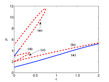
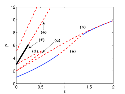
Figure 1: (Color online) Top: The power versus the coupling strength for solution of types (a)–(e) from Table 1 for the nearest-neighbor (local) DNLS equation, i.e. with $k_{2}=0$. Dashed red and solid blue lines correspond to unstable and stable solutions, respectively. Bottom: The same branches in the NNN DNLS equation, with $k_{2}=0.6$. Solution (f) with a nontrivial phase distribution (black thicker part of the line) appears in the latter case, with power which is very close to that of solution (e) with the trivial phase distribution. This bifurcation can be better seen by comparing the phases, see Fig. 3. The unlabeled (top) branch (which corresponds to initial phases of $\{0,0,\pi,0,0\}$) merges with the branch labeled (e) in both panels (although the collision occurs outside the plotting region for the bottom panel).

2.4 Bifurcations

From Eq. (6) we see that in the standard nearest-neighbor DNLS equation, only solutions with trivial phase distributions persist for non-zero coupling. These solutions can be continued in $\epsilon$ and gradually vanish through saddle-node bifurcations [10], with only the single-site ($\theta_{0}=0$) and two-site ($\theta_{0}=\theta_{1}=0$) solutions persisting toward the continuum limit (with both approaching the soliton solution of the continuous NLS equation). This bifurcation scenario is shown in the top panel of Fig. 1 for configurations (a)–(e) of Table 1. The extended coupling allows for additional types of solutions with nontrivial phase patterns, which, in the case of the NNN system, means one additional waveform, indicated by the thick black solid line in the bottom panel of Fig. 1. In these diagrams, the power is plotted versus coupling strength $\epsilon$. For this choice of parameters, the nontrivial branch (f) and the trivial one (e) lie very close to each other, making the identification of the bifurcation points difficult. The role of the nontrivial-phase solutions can be better seen through the comparison of the phases, see below Figs. 3 and 4. Also, the extended coupling modifies the stability properties of some trivial phase solutions. For example, the branch (a) is always stable for the nearest-neighbor interactions (see top panel of Fig. 1) while it displays an instability window for intermediate coupling strengths in the NNN coupling case (see bottom panel of Fig. 1), in a way somewhat reminiscent of the findings of [3, 4].

3 The Variational Approximation

The Lagrangian of Eq. (4) is

$$\mathcal{L}=\sum_{n\in{\mathbb{Z}}}\left[\frac{1}{2}|\phi_{n}|^{4}-|\phi_{n}|^{2}+\epsilon\sum_{m\in S}k_{nm}\phi_{n}^{\ast}\phi_{m}\right].$$ (10)

According to the variational principle, critical points of the Lagrangian (10) correspond to solutions of Eq. (4). This underlies the heuristic justification of the variational approximation (VA), whereby an ansatz (trial configuration of the wave field) with a finite number of parameters is substituted into the Lagrangian, and critical points are then sought for the resulting finite parameter subspace. This approach has long been used in various applications, see the review [11] and more recent works, such as Refs. [12, 13, 14]. The VA has also been used to study nonlocal interactions, see, e.g., Ref. [4], but in the latter case only solutions initiated by a single excited site in the AC limit, i.e., solutions of type (a) in terms of Table 1, were studied. To the best of our knowledge, the present work for the first time extends the VA to describe not only discrete multi-humped solutions with arbitrary phases (with at least three excited sites), but also ones such with nontrivial phase distributions.

3.1 Trivial Phase Distributions

We start by considering solutions with nontrivial phase distributions. Our objective is to construct approximate discrete solitons by means of a real-valued ansatz:

$$\begin{array}[]{ll}\psi_{n}&=\left\{\begin{array}[]{ll}B_{n}~{}\mathrm{for}&n\in S,\\ A\exp(-\eta|n+n_{0}|)~{}\mathrm{for}&n\notin S,\end{array}\right.\\[8.61108pt] &\end{array}$$ (11)

where $S$ denotes the set of nodes between the first and last excited lattice sites. We define the width $W$ of the solution as the number of elements of the set $S$. Parameters $A$ and $B_{n}$ represent the amplitudes, and $\eta$ is the decay rate. For solutions with odd $W$ (site-centered configurations) the position parameter is $n_{0}=0$, and for even $W$ (bond-centered configurations) it is $n_{0}=0.5$. Independent amplitudes $B_{n}$ are necessary to describe the core of the multi-humped solutions accurately.

Since this ansatz is genuinely discrete and includes a purely exponential tail, the corresponding approximations will only be valid for a small coupling strength, since the solutions become increasingly smooth (sech-like) as the continuum limit is approached. On the other hand, solutions with a single excited site in the AC limit are only weakly influenced by the extended coupling. For this reason, we aim to apply the VA to the simplest solution type that “feels” the extended coupling, which corresponds to $W=3$. The substitution of this ansatz into the Lagrangian and calculation of the ensuing sums yields the effective Lagrangian

$$\mathcal{L}_{\mathrm{eff}} = \frac{A^{4}}{2}E_{0,2\eta}-A^{2}E_{0,\eta}+\sum_{m\in{\mathbb{N}}}\epsilon A^{2}E_{m,\eta}k_{|m|}$$

$$-\sum_{j\in S}\left[B_{j}^{2}(1-B_{j}^{2}/2)-\epsilon\sum_{n=-W}^{W}k_{j}\psi_{n}^{\ast}\psi_{j}\right],$$

where

$$E_{j,\eta}\equiv\frac{e^{-\eta(2+|j|)}}{e^{2\eta}-1}.$$ (13)

The Euler-Lagrange equations derived from this Lagrangian are

$$\frac{\partial\mathcal{L}_{\mathrm{eff}}}{\partial p_{i}}=0,$$ (14)

where $p_{i}\in\{A,B_{n}\}$ are parameters of the ansatz. The equation corresponding to varying amplitude $A$ yields

$$2A^{3}E_{0,2\eta}-2AE_{0,\eta}+\epsilon 2A\sum_{m\in{\mathbb{N}}}E_{m,\eta}k_{m}+e^{-3\eta}\epsilon(B_{-1}+B_{1})k_{2}$$

$$+2e^{-2\eta}\epsilon(2B_{0}k_{2}+(B_{-1}+B_{1})k_{1})=0,$$ (15)

and the variation of the $B_{j}$’s yields,

$$B_{-1}(B_{-1}^{2}-1)+\epsilon\left(Ae^{-3\eta}k_{2}+Ae^{-2\eta}k_{1}+{\sum_{m\in{\mathbb{N}}}}^{\prime}k_{|m|}B_{|m|-1}\right) = 0,$$ (16)

$$B_{0}(B_{0}^{2}-1)+\epsilon\left(2Ae^{-2\eta}k_{2}+k_{0}B_{0}+k_{1}(B_{-1}+B_{1})\right) = 0,$$ (17)

$$B_{1}(B_{1}^{2}-1)+\epsilon\left(Ae^{-3\eta}k_{2}+Ae^{-2\eta}k_{1}+{\sum_{m\in{\mathbb{N}}}}^{\prime}k_{|m|}B_{1-|m|}\right) = 0,$$ (18)

where the prime over the sum indicates that the $m=0$ entry is to be doubled.

Rather than performing the variation with respect to decay constant $\eta$, we replace it by $\eta\equiv\ln\lambda$, where $\lambda$ is the corresponding multiplier determined by the dynamical reduction. Furthermore, we set $n_{0}=0$ rather than using it as a variational parameter. This excludes asymmetric solutions, hence we can also set $B_{1}=B_{-1}$, further reducing the number of parameters.

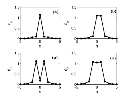
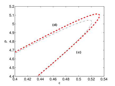
Figure 2: Top panels: Numerical solutions of Eq. (1) with trivial phase distributions (solid lines) and the variational solutions based on ansatz (11) continued to $\epsilon=0.1$ (markers). Labels (a)–(d) correspond to those in Table 1. The error $\|\phi-\psi\|_{l^{2}}$ at these parameter values are (a) $7.4\times 10^{-5}$ , (b) .0009, (c) .002, and (d) .001. Middle panel: Zoom of the saddle-node bifurcation involving branches (c) and (d) from the bottom panel of Fig. 1. The variational solution (the black dash-dotted line) predicts the bifurcation at a slightly smaller value of the coupling strength than the numerical solution (the red dashed line). Both solutions are unstable in this parameter region. Bottom panel: Plot of two pairs of isolated eigenvalues versus the arc length of the $P(\epsilon)$ curve of the middle panel. Here, zero arc length corresponds to the (c) solution at $\epsilon=0$ and the end of the arc length curve corresponds to the (d) solution at $\epsilon=0$. The eigenvalue pair (I) emerges from the edge of the continuous spectrum, i.e. $\lambda^{2}=-1$. The eigenvalue pair (II) is responsible for the instability since it has positive real part (i.e. $\lambda^{2}>0$ ) in the entire region plotted.

Equations (16)–(18) pertain to the localized pattern with $W=3$, but they can be readily extended to other cases. Using these equations, we can approximate all the solutions with trivial phases from Fig. 1, i.e., branches (a)–(e), including the single- and double-site solutions, see the top panel of Fig. 2. Indeed, the predictions are so good that one cannot see the differences when the bifurcation diagram based on the VA is juxtaposed with Fig. 1. A zoom of the saddle-node bifurcation between solutions (c) and (d) is shown in the bottom panel of Fig. 2 where the differences are visible. One might expect the (c) and (d) solutions to exchange stability, which would be the case in a standard saddle-node bifurcation in a low-dimensional model. However, due to the higher dimensionality of the DNLS model considered here, there will be additional eigenvalues that could affect the stability character of the solution. Indeed, for the (c) and (d) solutions there are two pairs of isolated eigenvalues (and one pair at the origin). One of these pairs moves along the imaginary axis and becomes real (see curve (I) of the bottom panel of Fig. 2) for some critical value of $\epsilon$. However, due to the existence of the other pair of eigenvalues (see curve (II)), which has non-zero real part in the parameter region shown, both solutions are unstable.

It is obvious that ansatz (11) can only capture solutions with the trivial phase structure, as it is real-valued. Nonetheless, it is informative to inspect the AC limit in the framework of the variational equations to see what types of solutions are candidates to be approximated. With $\epsilon=0$ the equations reduce to $A=0$ and $B_{j}(B_{j}^{2}-1)=0$ such that the corresponding VA solutions coincide exactly with solutions of the full problem (4) with the phases given by either $0$ or $\pm\pi$, as expected. The fact that the VA and full solutions match at $\epsilon=0$ follows from the choice of the ansatz. This is not the case if the standard ansatz, based on the exponential cusp with the single central point is used, cf. Ref. [16].

3.2 Nontrivial Phase Distributions

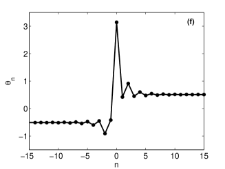
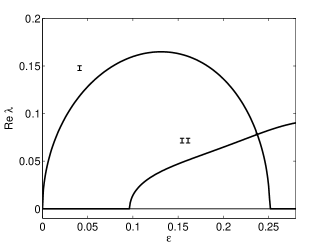
Figure 3: (Color online) Left: Phases of the nontrivial solution (f) for $\epsilon=0.1$ and the same parameter values as in Table 1. Middle: Phases at the $n=\pm 1$ and $n=0$ sites for versus $\epsilon$. Solution (e) corresponds to $\theta_{-1}=\theta_{1}=0$ and $\theta_{0}=\pi$ (red dashed lines) while solution (f) corresponds $\theta_{0}=\pi$ and nontrivial $\theta_{\pm 1}$ (blue solid curves). The solutions (e) and (f) collide at the critical point, $\epsilon\approx 0.25$, where the latter terminates through the ensuing subcritical pitchfork bifurcation. Right: The two eigenvalues with the largest real part, found from a solution of Eq. (9) corresponding to solution (e). The eigenvalue corresponding to the bifurcation shown in the middle panel is labeled I. However, due to the emergence of a second real eigenvalue pair (II), the solution (e) is unstable in all of the parameter region shown. The corresponding spectral picture for the solution (f) is similar, but without the curve I. Thus, solution (f) becomes unstable at $\epsilon\approx 0.098$.

In order to capture solutions with nontrivial phases, phase must be added to the ansatz. To motivate our choice, we look closer at the solutions with nontrivial phases. Similarly to the trivial-phase ansatz (11), we separate the initially excited sites from the others. The outer part of the solution should have exponential decay, but with a varying phase. In the left panel of Fig. 3 the phases of the numerically found nontrivial solution (f) for $\epsilon=0.1$ are plotted against the lattice coordinate. A precise description of each phase would make the ansatz too complex, leading to intractable sums in the effective Lagrangian. However, it is clear that the solution will be an exponentially localized one, and a coarse approximation for the phases may be sufficient. Therefore, motivated by Fig. 3, we assume a constant phase, $\kappa_{-1}$, for $n<0$ and another constant phase, $\kappa_{1}$, for $n>0$. For the core of the solution, one might introduce the number of additional phase parameters equal to $W$, one per each site, but, aiming to keep the number of parameters reasonably low, we make the following observations based on the dependence of the phases for the core sites as a function of $\epsilon$ (see middle panel of Fig. 3). We have observed that the phase at the central site ($n=0$) stays almost constant as the coupling is turned on and the difference between the other points in the core ($n=\pm 1$) are $\theta_{\pm 1}(\epsilon)\approx\theta_{\pm 1}^{0}\pm b$, where $\theta_{n}^{0}$ is the phase at the $n$-th site in the AC limit, and $b$ is a constant which depends on parameters of the system (see the middle panel of Fig. 3). Therefore, for the nontrivial-phase solution with width $W=3$ we adopt the following ansatz,

$$\psi_{n}=\left\{\begin{array}[]{ll}A\exp(\mathrm{i}\kappa_{-1})\exp(-\eta|n|)&\mathrm{~{}for~{}}n<-1,\\[4.30554pt] B\exp(\mathrm{i}(\phi_{-1}^{0}-b))&\mathrm{~{}for~{}}n=-1,\\[4.30554pt] C\exp(\mathrm{i}\phi_{0}^{0})&\mathrm{~{}for~{}}n=0,\\[4.30554pt] B\exp(\mathrm{i}(\phi_{1}^{0}+b))&\mathrm{~{}for~{}}n=1,\\[4.30554pt] A\exp(\mathrm{i}\kappa_{1})\exp(-\eta|n|)&\mathrm{~{}for~{}}n>1,\end{array}\right.$$ (19)

where real parameters $A,B,C$ represent the amplitude, and the phases are represented by $\kappa_{\pm 1}$ and $b$. As before, $\eta$ is determined via the dynamical reduction. We also present in the right panel of Fig. 3 the instability eigenvalues for the trivial phase solution (e). As can be seen from this panel, if it was not for the eigenvalue pair (II), this solution would gain stability after collision with the nontrivial phase solution (f) for $\epsilon>0.25$. In particular, this eigenvalue plot in conjunction with the middle panel of the figure illustrating the phases of the different branches clearly showcases the existence of a subcritical pitchfork bifurcation, which leads to the termination of the nontrivial phase branch (f).

The effective Lagrangian corresponding to the nontrivial-phase ansatz is the same as in the case of the solution with the trivial phases, with the exception that $\psi$ appearing in Eq. (14) will be the one of Eq. (19) and with $B_{\pm 1}=B$ and $B_{0}=C$.

The variation of the effective Lagrangian with respect to the parameters $A,B,C,\kappa_{-1},\kappa_{1}$ and $b$ yields, respectively,

$$0 = -2AE_{0,\eta}+B\epsilon(k_{1}e^{-2\eta}+k_{2}e^{-3\eta})(\cos(r^{-})+\cos(r^{+}))+\epsilon e^{-2\eta}Ck_{2}(\cos(\kappa_{-1}-\theta_{0}^{0})+\cos(\kappa_{1}-\theta_{0}^{0}))$$ (20)

$$+\epsilon 2A\sum_{m\in S}E_{m,\eta}k_{m}+2A^{3}E_{0,2\eta},$$

$$0 = \epsilon Bk_{2}\cos(\theta_{-1}^{0}+2b-\theta_{1}^{0})+\epsilon(Ck_{1}(\cos(s^{-})+\cos(s^{+}))+A(\cos(r^{-})+\cos(r^{+}))(k_{1}e^{-2\eta}+k_{2}e^{-3\eta}))$$ (21)

$$+B(B^{2}-1)+\epsilon Bk_{0},$$

$$0 = \epsilon(Ck_{0}+Bk_{1}(\cos(s^{-})+\cos(s^{+}))+Ak_{2}e^{-2\eta}(\cos(\theta_{0}^{0}+\kappa_{-1})+\cos(-\theta_{0}^{0}+\kappa_{1})))+C(C^{2}-1),$$ (22)

$$0 = \epsilon A(Ck_{2}e^{-2\eta}\sin(\kappa_{-1}-\theta_{0}^{0})+B\sin(r^{-})(k_{1}e^{-2\eta}+k_{2}e^{-3\eta})),$$ (23)

$$0 = \epsilon A(Ck_{2}e^{-2\eta}\sin(\kappa_{1}-\theta_{0}^{0})+B\sin(r^{+})(k_{1}e^{-2\eta}+k_{2}e^{-3\eta})),$$ (24)

$$0 = \epsilon B(2A(\sin(r^{+})-\sin(r^{-}))(k_{1}e^{-2\eta}+k_{2}e^{-3\eta})-4k_{2}B\sin(\theta_{0}^{0}+2b-\theta_{-1}^{0}))$$ (25)

$$-\epsilon BCk_{1}(\sin(s^{+})-\sin(s^{-})),$$

where $r^{-}\equiv\kappa_{-1}-b-\theta_{-1}^{0}$,$~{}r^{+}\equiv\kappa_{1}+b-\theta_{1}^{0}$, $s^{-}=-\theta_{-1}^{0}-b+\theta_{0}^{0}$, and $s^{+}=-\theta_{1}^{0}+b+\theta_{0}^{0}$. These equations reduce to those for the trivial-phase solutions, displayed in the previous section for $\kappa_{\pm 1}=0$ and $b=\theta_{1}^{0}$. To look at the bifurcation between the trivial- and nontrivial-phase solutions (e) and (f) in another way, we can vary the outer coupling parameter $k_{2}$ in Eq. (5), while keeping $\epsilon$ fixed. As mentioned before, it is easier to identify the bifurcation through the comparison of phases, therefore we consider the phase difference $\Delta\theta=\theta_{0}-\theta_{1}$, which has the advantage of being independent of any constant phase (since the solutions are gauge invariant). The agreement between the numerically exact solution and the one based on the VA is quite remarkable, see the bottom panel of Fig. 4. In this panel, the mirror symmetric nontrivial phase solution (i.e., the one with opposite relative phases) has been omitted.

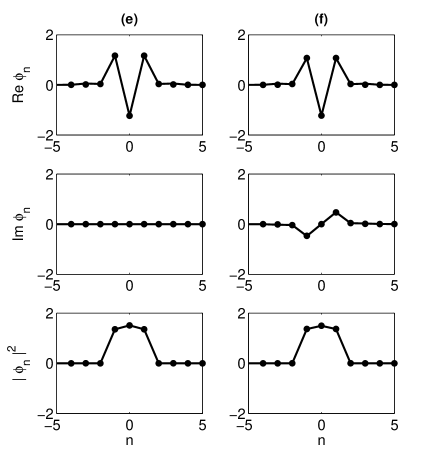
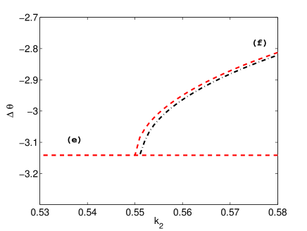
Figure 4: Top panels: The real part (top row) and imaginary part (middle row) of the trivial-phase solution (e) and the one with the nontrivial phase (f). The numerically exact solutions (solid lines) are close to their variational counterparts (markers) based on ansatz (19), with errors $\|\phi-\psi\|_{l^{2}}$ being .004 (e) and .004 (f). The parameters are again the same as in Table 1 and $\epsilon=1$. Bottom panel: Phase difference $\Delta\theta=\theta_{0}-\theta_{1}$ for the numerical (red dashed curve) and variational (black dash-dotted curve) solutions for branches (e) and (f) versus the outer-coupling parameter $k_{2}$ for $\epsilon=0.1$. The bifurcation here is of the pitchfork type, with the mirror-symmetric partner of (f) connecting with solution (e) as well.

Using these variational equations, it is possible to approximate the bifurcation point in the bottom panel of Fig. 4 which connects solutions (e) and (f) without actually solving Eqs. (20)–(25). Making use of the approximations $\kappa_{1}=-\kappa_{-1}$ and $\kappa_{-1}=(b+\theta_{-1})/2$ and Taylor-expanding Eq. (23) leads to

$$\kappa_{-1}\approx\pm\sqrt{\frac{B(k_{1}e^{-2\eta}+k_{2}e^{-3\eta})-2Ck_{2}e^{-2\eta}}{B(k_{1}e^{-2\eta}+k_{2}e^{-3\eta})/12-2Ck_{2}e^{-2\eta}/96}},$$ (26)

or $\kappa_{-1}=0$. Using values of $B$ and $C$ obtained from the (much simpler) equations (15)–(18), we thus produce an accurate prediction of the bifurcation, avoiding the need to solve the full system of Eqs. (20)–(25), since all terms in Eq. (26) are known. The right hand side of equation (26) vanishes at $k_{2}\approx 0.538$, which is close the actual bifurcation value of $k_{2}\approx 0.551$ in Fig. 4. This is an improvement in comparison to the prediction based on Eq. (6), which is $k_{2}\approx 0.5$. The deviation from the latter simple leading order prediction can be justified by the use of $\epsilon=1$, whereas the derivation of [2] was valid for small $\epsilon$.

As a final example, we will briefly consider a four-site solution $(W=4)$. The corresponding even counterpart of ansatz (19) is

$$\psi_{n}=\left\{\begin{array}[]{ll}A\exp(\mathrm{i}\kappa_{-1})\exp(-\eta|n+n_{0}|)&{\rm~{}for~{}}n<-1\\[4.30554pt] B\exp(\mathrm{i}(\phi_{-1}^{0}-b))&{\rm~{}for~{}}n=-1\\[4.30554pt] C\exp(\mathrm{i}(\phi_{0}^{0}-c))&{\rm~{}for~{}}n=0\\[4.30554pt] C\exp(\mathrm{i}(\phi_{1}^{0}+c))&{\rm~{}for~{}}n=1\\[4.30554pt] B\exp(\mathrm{i}(\phi_{1}^{0}+b))&{\rm~{}for~{}}n=2\\[4.30554pt] A\exp(\mathrm{i}\kappa_{1})\exp(-\eta|n+n_{0}|)&{\rm~{}for~{}}n>2,\end{array}\right.$$ (27)

where $n_{0}=0.5$. The effective Lagrangian corresponding to ansatz (27) is the same as the trivial-phase one, with the exception that once again the $\psi$ appearing in Eq. (14) will be of the form of Eq. (27), with $B_{-1}=B_{2}=B$, $B_{0}=B_{1}=C$, and

$$E_{j,\eta}=\frac{e^{-\eta(2+|j|+2n_{0})}+e^{-\eta(4+|j|+2n_{0})}}{e^{2\eta}-1}.$$ (28)

The extra term $e^{-\eta(4+|j|+2n_{0})}$ appearing in the expression for $E_{j,\eta}$ for the solutions with the even width is due to the fact the summation in the Lagrangian is no longer symmetric about the zero site. The variations with respect to the parameters $A,B,C,\kappa_{-1},\kappa_{1},b$ and $c$ yield, respectively,

$$0 = A^{3}E_{0,2\eta}-AE_{0,\eta}+\epsilon A\sum_{m\in S}E_{m,\eta}k_{m}+\epsilon B\left(k_{1}e^{-\eta(2+n_{0})}+k_{2}e^{-\eta(3+n_{0})}\right)\cos(r_{b}^{-})$$

$$+\epsilon B\left(k_{1}e^{-\eta(3+n_{0})}+k_{2}e^{-\eta(4+n_{0})}\right)\cos(r_{b}^{+})+\epsilon Ck_{2}e^{-\eta(2+n_{0})}\cos(r_{c}^{-})+\epsilon Ck_{2}e^{-\eta(3+n_{0})}\cos(r_{c}^{+}),$$

$$0 = 2B(B^{2}-1)+2\epsilon Bk_{0}+\epsilon Ck_{1}(\cos(s_{c}^{-})+\cos(s_{c}^{+}))+\epsilon Ck_{2}(\cos(s_{b}^{-})+\cos(s_{b}^{+}))$$

$$+\epsilon A\left(\cos(r_{b}^{-})k_{1}e^{-\eta(2+n_{0})}+\cos(r_{b}^{-})k_{2}e^{-\eta(3+n_{0})}+\cos(r_{b}^{+})k_{1}e^{-\eta(3+n_{0})}+\cos(r_{b}^{+})k_{2}e^{-\eta(4+n_{0})}\right),$$

$$0 = 2C(C^{2}-1)+\epsilon B(k_{1}\cos(s_{c}^{-})+k_{1}\cos(s_{c}^{+})+k_{2}\cos(s_{b}^{-})+k_{2}\cos(s_{b}^{+}))+2\epsilon Ck_{0}$$

$$+2\epsilon Ck_{1}\cos(\theta_{0}+2c-\theta_{1})+\epsilon Ak_{2}(e^{-\eta(2+n_{0})}\cos(\theta_{0}-\kappa_{-1}+c)+e^{-\eta(3+n_{0})}\cos(\theta_{1}-\kappa_{1}-c)),$$

$$0 = \epsilon A(Ck_{2}e^{-\eta(2+n_{0}))}\sin(\kappa_{-1}-\theta_{0}^{0}-c)+B\sin(r_{b}^{-})(k_{1}e^{-\eta(2+n_{0})}+k_{2}e^{-\eta(3+n_{0})}),$$ (32)

$$0 = \epsilon A(Ck_{2}e^{-\eta(3+n_{0})}\sin(\kappa_{1}-\theta_{1}+c)+B\sin(r_{b}^{+})(k_{1}e^{-\eta(3+n_{0})}+k_{2}e^{-\eta(4+n_{0})}),$$ (33)

$$0 = -\epsilon BC(k_{2}\sin(s_{b}^{-})+k_{2}\sin(s_{b}^{+})+k_{1}\sin(s_{c}^{+})+k_{1}\sin(s_{c}^{-}))$$

$$+\epsilon BA\left(\sin(r_{b}^{-})k_{2}e^{-\eta(3+n_{0})}-\sin(r_{b}^{+})k_{2}e^{-\eta(4+n_{0})}-\sin(r_{b}^{+})k_{1}e^{-\eta(3+n_{0})}+\sin(r_{b}^{-})k_{1}e^{-\eta(2+n_{0})}\right),$$

$$0 = -\epsilon CB(k_{2}\sin(s_{b}^{-})+k_{2}\sin(s_{b}^{+})-k_{1}\sin(s_{c}^{+})-k_{1}\sin(s_{c}^{-}))-2k_{1}\epsilon C^{2}\sin(\theta_{0}-2c-\theta_{1})$$

$$+\epsilon AC\left(\sin(r_{c}^{-})k_{2}e^{-\eta(2+n_{0})}-\sin(r_{c}^{+})k_{2}e^{-\eta(3+n_{0})}\right),$$

where $r_{b}^{-}\equiv\kappa_{-1}-b-\theta_{-1}$, $r_{b}^{+}\equiv\kappa_{1}+b-\theta_{2}$, $r_{c}^{-}\equiv\kappa_{-1}-c-\theta_{0}$ and $r_{c}^{+}\equiv\kappa_{1}+c-\theta_{1}$, $s_{b}^{-}\equiv\theta_{-1}-\theta_{1}+c+b$, $s_{b}^{+}\equiv\theta_{0}-\theta_{2}+c+b$, $s_{c}^{-}\equiv\theta_{1}-\theta_{2}-c+b$, $s_{c}^{+}\equiv\theta_{-1}-\theta_{0}-c+b$. Although it is not the goal of this work to provide for a list of every possible bifurcation scenario, it is worth mentioning that nontrivial-phase solutions connect various types of phase-trivial ones. For example, as depicted in Fig. 5, the nontrivial solution (h) connects the phase-trivial ones (g) and (i), with $k_{2}$ treated as the bifurcation parameter. Solution (g), with phases differences $\{\Delta\theta_{1},\Delta\theta_{2}\}=\{-\pi,-\pi\}$, bifurcates at $k_{2}\approx 0.345$, where the nontrivial-phase solution (h) emerges. The phase differences of solution (h) change as $k_{2}$ varies. At $k_{2}\approx 0.894$, solution (h) collides with and is annihilated by the trivial-phase solution (i), which has phases differences $\{\Delta\theta_{1},\Delta\theta_{2}\}=\{0,-\pi\}$. I.e., the phenomenology involves a supercritical pitchfork (in the bifurcation parameter $k_{2}$) for the emergence of the nontrivial phase branch (h) from (g) and a subcritical pitchfork which results from the collision of (g) with (i). This is similar to how asymmetric solutions connect solutions of varying width in DNLS equations with higher-order nonlinearities [14, 17, 18, 19] with the exception that the overall (in)stability of the trivial-phase solutions is not affected by collision with nontrivial-phase solutions. The nontrivial-phase solution itself undergoes stability change, as can be seen in the bottom panel of Fig. 5. The VA captures this scenario remarkably well. Indeed, in the top subpanel of the bottom panels in Fig. 5, the difference between the numerical and variational solutions cannot be spotted. Actually, a very strong zoom around the bifurcation point is needed to depict the difference (see bottom subpanel) and the relevant error in the identification of the critical point is less than $0.4$ $\%$.

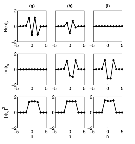
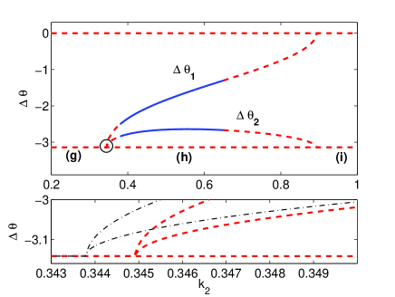
Figure 5: (Color online) Top six panels: Profiles of the four-site trivial-phase solutions (g) and (i), which are connected through the nontrivial phase solution (h). Bottom two panels: Plots of the phases differences $\Delta\theta_{1}=\theta_{1}-\theta_{0}$ and $\Delta\theta_{2}=\theta_{2}-\theta_{1}$ of solutions (g)–(i). At the resolution of the top subpanel the difference between the variational and numerical curves cannot be seen. Solution (h) undergoes two stability changes in the parameter region shown here (dashed red and blue solid lines show the unstable and stable families, respectively). Bottom subpanel: Zoom of the circled area showing the discrepancy between the variational approximation (black dash-dotted lines) and numerically generated curves (red dashed lines).

4 Conclusions

We have revisited discrete nonlinear Schrödinger (DNLS) models with extended linear couplings in the lattice, developing a new version of the variational approximation (VA) for the models of this type. Using an ansatz that coincides with exact solutions in the anti-continuum limit, we were able to accurately describe, for the first time, multi-humped solutions, including those with nontrivial phase structures, and the bifurcations linking different species of the discrete solitons. Pitchfork bifurcations connecting the solutions with the nontrivial and trivial phase structures were identified, which the VA was successful in predicting, thus demonstrating its reliability. In particular, the strength of VA analysis is that it provides simple formulas to predict such bifurcation points. Like in other settings where the VA is used, a precise evaluation of the validity of this approximation is an open question, therefore we relied on the direct comparison with numerical solutions of the full problem. It was found that the accuracy of the VA is quite good for small lattice coupling strength.

There remain several other open problems concerning next-nearest-neighbor DNLS equations, such as how to compute the stable manifolds in terms of the dynamical reduction, or what the appropriate continuum-limit counterparts of these models are and what modifications to the existence and spectral properties of the solitary waves the long-range kernels may induce more generally. As concerns the VA, its time-dependent version can be also used to predict the linear stability of the solutions, see Refs. [11] and [14], which may be another direction for the development of the analysis reported in this work. Finally, bearing in mind some of the important consequences of long-range interactions in higher dimensions, such as the stabilization of unstable vortices among others [20], consideration of such questions in the discrete realm is a theme of particular interest in its own right.

References

- [1] P.G. Kevrekidis, The discrete nonlinear Schrödinger equation: Mathematical analysis, numerical computations and physical perspectives, Springer, New York, 2009.
- [2] P.G. Kevrekidis, Non-nearest-neighbor interactions in nonlinear dynamical lattice, Phys. Lett. A 373 (2009) 3688–3693.
- [3] Y.B. Gaididei, S.F. Mingaleev, P.L. Christiansen, and K.Ø. Rasmussen, Effects of nonlocal dispersive interactions on self-trapping excitations, Phys. Rev. E 55 (1997) 6141–6150.
- [4] K.Ø. Rasmussen, P.L. Christiansen, Y.B. Johansson, M. Gaididei, and S.F. Mingaleev, Localized excitations in discrete nonlinear Schrödinger systems: Effects of nonlocal dispersive interactions and noise, Physica D 113 (1998) 134–151.
- [5] D.N. Christodoulides and N. Efremidis, Discrete solitons in nonlinear zigzag optical waveguide arrays with tailored diffraction properties, Phys. Rev. E 65 (2002) 056607.
- [6] S.F. Mingaleev, P.L. Christiansen, Y.B. Gaididei, M. Johansson, and K.Ø. Rasmussen, Models for energy and charge transport and storage in biomolecules, J. Biol. Phys. 25 (1999) 41–63.
- [7] J. Cuevas, G. James, P.G. Kevrekidis, B.A. Malomed, and B. S nchez-Rey, Approximation of solitons in the discrete NLS equation, J. Nonlinear Math. Phys. 15 (2008) 124–136.
- [8] T. Kapitula, P.G. Kevrekidis, and B.A. Malomed, Stability of multiple pulses in discrete systems. Phys. Rev. E 63 (2001) 036604.
- [9] D.E. Pelinovsky, P.G. Kevrekidis and D. Frantzeskakis, Stability of discrete solitons in nonlinear Schrödinger lattices, Physica D 212 (2005) 1–19.
- [10] G.L. Alfimov, V.A. Brazhnyi, and V.V. Konotop, On classification of intrinsic localized modes for the discrete nonlinear Schrödinger equation, Physica D 194 (2004) 127–150.
- [11] B.A. Malomed, Variational methods in nonlinear fiber optics and related fields, Progr. Opt. 43 (2002) 71–193.
- [12] D.J. Kaup and B.A. Malomed, Embedded solitons in Lagrangian and semi-Lagrangian Systems, Physica D 184 (2003) 153–161.
- [13] D.J. Kaup, Variational solutions for the discrete nonlinear Schrödinger equation, Math. Comput. Simulat. 69 (2005) 322–333.
- [14] C. Chong and D.E. Pelinovsky, Variational approximations of bifurcations of asymmetric solitons in cubic-quintic nonlinear Schrödinger lattices, Disc. Cont. Dyn. Syst. S, 4 (2011) 1019–1032
- [15] C. Chong, R. Carretero-González, B.A. Malomed, and P.G. Kevrekidis. Multistable Solitons in Higher-Dimensional Cubic-Quintic Nonlinear Schrödinger Lattices. Physica D, 238 (2009) 126–136.
- [16] B.A. Malomed and M.I. Weinstein, Soliton dynamics in the discrete nonlinear Schrödinger equation, Phys. Lett. A 220 (1996) 91–96.
- [17] R. Carretero-González, J.D. Talley, C. Chong, B.A. Malomed, Multistable solitons in the cubic-quintic discrete nonlinear Schrödinger equation, Physica D 216 (2006) 77–89.
- [18] M.Öster, M. Johansson, A. Eriksson, Enhanced mobility of strongly localized modes in waveguide arrays by inversion of stability, Phys. Rev. E 67 (2003) 056606.
- [19] C. Taylor and J.H.P. Dawes, Snaking and isolas of localised states in bistable discrete lattices, Phys. Lett. A 375 (2010) 4968–4976.
- [20] D. Briedis, D.E. Petersen, D. Edmundson, W. Krolikowski and O. Bang, Ring vortex solitons in nonlocal nonlinear media, Opt. Express 13 (2005) 435–443.