UT-11-03 TIT/HEP-608 Feb 2011 Superconformal index for large $N$ quiver Chern-Simons theories

We investigate the ${\cal N}=2$ superconformal index for supersymmetric quiver Chern-Simons theories with large $N$ gauge groups. After general arguments about the large $N$ limit, we compute the first few terms in the series expansion of the index for theories proposed as dual theories to homogeneous spaces $V^{5,2}$, $Q^{1,1,1}$, $Q^{2,2,2}$, $M^{1,1,1}$, and $N^{0,1,0}$. We confirm that the indices have symmetries expected from the isometries of dual manifolds.

1 Introduction

The field-operator correspondence is an important prediction of AdS/CFT[1]. It claims a one-to-one correspondence between gauge invariant operators in a conformal field theory and excitations in the dual geometry including supergravity Kaluza-Klein modes and extended objects. It is, in general, difficult to compute the operator spectrum on the gauge theory side due to quantum corrections. However, in supersymmetric theories, it is often possible to obtain exact results even in the strong coupling region. For example, in many superconformal field theories, we can exactly compute superconformal index, which has rich information of the BPS spectrum. The agreement of the superconformal index on both sides of the duality provides a strong evidence for the duality.

The ${\cal N}=1$ superconformal index for four-dimensional gauge theories is used as a test of AdS/CFT correspondence for ${\cal N}=4$ supersymmetric Yang-Mills theory in [2]. The agreement of indices on both sides was confirmed to leading order in the large $N$ limit. It has been extended to theories with less supersymmetries [3, 4, 5, 6, 7, 8, 9, 10].

Indices are also applied for analysis of AdS₄/CFT₃. For the ABJM model[11] the ${\cal N}=2$ superconformal index is computed in the perturbative sector[12], which does not contain monopole operators. It is confirmed that the gauge theory index agrees with that on the gravity side. This analysis is extended into monopole sectors in [13], and the agreement is again confirmed. Similar analysis is performed for ${\cal N}=3,4,5$ Chern-Simons theories in [14, 15, 16].

The ${\cal N}=2$ superconformal index is defined by[12]

$$I(x,z_{i})=\mathop{\rm tr}\nolimits\left[(-1)^{F}x^{\prime\{Q,Q^{\dagger}\}}x^{\Delta+j_{3}}z_{i}^{F_{i}}\right],$$ (1)

where the trace is taken over local gauge invariant operators. $Q$ is a nilpotent supercharge, which is used for the localization. $\Delta$, $j_{3}$, and $F_{i}$ are the dilatation, the third component of the spin, and flavor charges. Our choice of $Q$ is such that it has the quantum numbers $\Delta=+1/2$, $R=+1$, and $j_{3}=-1/2$. Only BPS states saturating the BPS bound

$$\{Q,Q^{\dagger}\}=\Delta-R-j_{3}\geq 0$$ (2)

contribute to the index. Therefore, it does not depend on $x^{\prime}$ appearing on the right hand side in (1).

In the previous works the canonical conformal dimension of fields are assumed in computations of the index by using the localization technique. This is the case for ${\cal N}\geq 3$ Chern-Simons theories because of non-abelian R-symmetry. It is recently extended to ${\cal N}=2$ superconformal field theories with arbitrary R-charge assignments[17]. The purpose of this paper is to rewrite the formula in [17] in a form applicable to large $N$ quiver Chern-Simons theories, and to compute the index for some examples of quiver Chern-Simons theories which are proposed as dual theories to homogeneous $7$-dimensional Sasaki-Einstein manifolds (SE₇) $V^{5,2}$, $Q^{1,1,1}$, $Q^{2,2,2}$, $M^{1,1,1}$, and $N^{0,1,0}$. See [18] and references therein for geometric properties of these manifolds.

We consider ${\cal N}=2$ superconformal quiver Chern-Simons theories with the gauge group of the form

$$G=\prod_{A=1}^{n_{G}}U(N)_{A},$$ (3)

and chiral multiplets belonging to bi-fundamental representations. In §10 we also introduce flavors, chiral multiplets belonging to (anti-)fundamental representations. We denote the Chern-Simons levels by $k_{A}$. Namely, the action of the theory contains the Chern-Simons terms

$$\sum_{A=1}^{n_{G}}\frac{ik_{A}}{4\pi}\int\mathop{\rm tr}\nolimits\left(A_{A}dA_{A}-\frac{2i}{3}A_{A}A_{A}A_{A}\right).$$ (4)

In any example of Chern-Simons theory proposed as a dual to M-theory in a background AdS${}_{4}\times$SE₇, monopole operators play an important role. For the gauge group (3), we can define $n_{G}$ conserved magnetic charges of an operator by

$$m_{A}=\frac{1}{2\pi}\oint\mathop{\rm tr}\nolimits F_{A},$$ (5)

where $F_{A}$ is the $U(N)_{A}$ gauge field strength, and the integration is taken over a sphere enclosing the insertion point of the operator. $m_{A}$ is the monopole charge associated with $U(1)_{A}$, the diagonal subgroup of $U(N)_{A}$. In theories without flavors, the magnetic charges are constrained by Gauss’ law constraint

$$\sum_{A=1}^{n_{G}}k_{A}m_{A}=0.$$ (6)

The constraint (6) decreases the number of independent magnetic charges by one, and we have $n_{G}-1$ independent magnetic charges. If the theory has the gravity dual, there should exist corresponding $n_{G}-1$ charges on the gravity side, too. In particular, monopole operators with the charge of the form

$$m_{1}=m_{2}=\cdots=m_{n_{G}}=m_{\rm diag}\in{\bf Z},$$ (7)

are known to correspond to Kaluza-Klein modes carrying momentum $m_{\rm diag}$ along the eleventh direction on the gravity side. We call such operators diagonal monopole operators. We need to assume

$$\sum_{A=1}^{n_{G}}k_{A}=0,$$ (8)

for the existence of diagonal monopole operators. The inclusion of diagonal monopole operators is essential for the emergence of the eleventh direction. The supergravity Kaluza-Klein spectrum in AdS${}_{4}\times$SE₇ is expected to agree with the spectrum of operators on the dual conformal field theory only if we include both perturbative operators consisting of elementary fields and diagonal monopole operators. The purpose of this paper is to obtain non-trivial evidences for this agreement by using the ${\cal N}=2$ superconformal index (1).

If $n_{G}\geq 3$, we also have non-diagonal monopole operators whose charge is not in the form (7). Such non-diagonal monopole operators correspond to M2-branes wrapped on two-cycles in SE₇[19]. When there exist BPS configurations of wrapped M2-branes, we should take account of them when we compute the index on the gravity side. This is the case in ${\cal N}=4$ Chern-Simons theories, whose dual geometries contain vanishing two-cycles[15]. M2-branes wrapped on such shrinking cycles contribute to the index. However, in examples we will consider in this paper all internal spaces do not have vanishing two-cycles. Non-vanishing two-cycles in SE₇ are non-BPS[20], and they should decouple in the computation of the index. Unfortunately, we have not succeeded in proving this decoupling on the gauge theory side, and in this paper we simply ignore the contribution of the non-diagonal monopole operators. In flavored theories, there may exist operators whose magnetic charges do not satisfy the constraint (6). We also ignore such operators, and we focus only on operators with diagonal magnetic charges.

We rely on a numerical method to obtain the index as the series expansion with respect to $x$. We compute the index in all examples up to the order of $x^{2}$. This is mainly because it takes much longer time to obtain higher order terms than ${\cal O}(x^{2})$.

This paper is organized as follows. In the next section, we write down the formula derived in [17] in the case of quiver Chern-Simons theories without flavors. In §3 and §4 we take the large $N$ limit and derive a formula for the index for vector-like theories. We apply it to a theory proposed as a dual theory to $V^{5,2}$ in §5, and confirm that the index has the symmetry which is expected from the isometry of $V^{5,2}$. In §6 we comment on the factorization of the index for chiral theories. We compute index for theories dual to $Q^{1,1,1}$, $Q^{2,2,2}$, and $M^{1,1,1}$ in §7, §8, and §9, respectively. We again confirm that in all cases the index has desirable symmetry. In §10 we extend the formula to theories with flavors, and in §11 we apply it to a theory dual to $N^{0,1,0}$. The last section summarizes the results.

2 Formula for the index

The index (1) can be defined as the path integral of the theory in the background ${\bf S}^{1}\times{\bf S}^{2}$ with appropriate boundary conditions. A formula for the index (1) is derived from this path integral with the help of localization method associated with the supercharge $Q$[13, 17]. If we deform the action by appropriate $Q$-exact terms, the path integral is localized at saddle points corresponding to GNO monopoles[21], which are Dirac monopoles for the Cartan part of the gauge group $G$. The magnetic charge of a GNO monopole is specified by a set of $\mathop{\rm rank}\nolimits G=n_{G}N$ integers, defined by

$$m_{A,i}=\frac{1}{2\pi}\oint_{{\bf S}^{2}}F_{A,i},$$ (9)

where $F_{A,i}$ is the $i$-th diagonal component of the $U(N)_{A}$ gauge flux $F_{A}$. The conserved charges defined in (5) are related to $m_{A,i}$ by

$$m_{A}=\sum_{i=1}^{N}m_{A,i}.$$ (10)

Note that $m_{A,i}$ are not conserved quantities, unlike $m_{A}$. We should regard them as integers labeling saddle points dominating the path integral. In addition to the monopole charges $m_{A,i}$, saddle points are also labeled by holonomy, denoted by $a$, which is the Wilson line around the ${\bf S}^{1}$. Namely, the saddle points form continuous sets in the configuration space. $m$ and $a$ take values in the Cartan part of the Lie algebra of the gauge group $G$.

We need to sum the contribution over all the saddle points. Let us denote this summation in a symbolic way by

$$\sum_{m}\int da.$$ (11)

$\sum_{m}$ is the summation over all independent magnetic charges. Here $m$ means a set of $n_{G}N$ magnetic charges $m_{A,i}$. We regard two magnetic charges transformed to each other by the Weyl Group of $G$ as being equivalent. By using this equivalence, we arrange the components of monopole charges in descending order in the set of $N$ components for each $U(N)$ gauge group. $\int da$ is given by

$$\int da=\frac{1}{(\mbox{stat})}\prod_{A=1}^{n_{G}}\prod_{\rho\in{\bf N}_{A}}\int\frac{d\rho(a)}{2\pi}=\frac{1}{(\mbox{stat})}\prod_{A=1}^{n_{G}}\prod_{i=1}^{N}\int\frac{da_{A,i}}{2\pi}.$$ (12)

We pick up a component of $a$ corresponding to a $U(1)$ subgroup of $U(N)_{A}$ by applying a weight $\rho\in{\bf N}_{A}$, where ${\bf N}_{A}$ is the fundamental representation of $U(N)_{A}$. $(\mbox{stat})$ is a numerical factor defined in the following way. Let us focus on one of $U(N)$ factors. In general, it is broken by the magnetic flux $m$ to its subgroup in the form

$$\prod_{i}U(N_{i})\subset U(N).$$ (13)

The order of the Weyl group of this unbroken symmetry is $\prod_{i}N_{i}!$. The statistical factor appearing in (12) is the product of this number for all $U(N)$ factors.

The trace in the definition of the superconformal index (1) represents the summation over all multi-particle states in ${\bf S}^{2}$, including single-particle states and the vacuum state. To compute the index (1), it is convenient to define the letter index

$$f(e^{ia},x,z_{i})=\sum(-1)^{F}e^{i\rho(a)}x^{\prime\Delta-R-j_{3}}x^{\Delta+j_{3}}z_{i}^{F_{i}}.$$ (14)

The letter index is defined for each monopole background, and the summation in (14) is taken over all single particle states on a GNO monopole background. The states summed over in (14) in general have non-vanishing gauge charges. We use the Wilson line $a$ as a chemical potential for the gauge charges. Once we obtain the letter index, the index for excitations including arbitrary number of particles is given as the plethystic exponential of the letter index

$$\exp\left[\sum_{n=1}^{\infty}\frac{1}{n}f(e^{ina},x^{n},z_{i}^{n})\right].$$ (15)

We also need to take account of the quantum numbers of the vacuum state, which are obtained by summing up the zero-point contribution of all single-particle states summed in (14). (Usually they diverge and we need suitable regularizations.) This is expressed in the form

$$P=e^{-S_{CS}}e^{ib_{0}(a)}x^{\epsilon_{0}}z_{i}^{q_{0i}}.$$ (16)

We call this a prefactor. $x^{\epsilon_{0}}$, $z_{i}^{q_{0i}}$, and $e^{ib_{0}(a)}$ correspond to the zero-point energy, zero-point flavor charges, and zero-point gauge charges, respectively, carried by the vacuum state. $S_{\rm CS}$ is the classical contribution from Chern-Simons terms (4),

$$S_{\rm CS}=i\sum_{A=1}^{n_{G}}\sum_{\rho\in{\bf N}_{A}}k_{A}\rho(a)\rho(m),$$ (17)

and has the effect of shifting gauge charges of the vacuum state.

We obtain the complete superconformal index by summing up the contribution of all saddle points[13, 17],

$$I(x,z_{i})=\sum_{m}\int daP\exp\left[\sum_{n=1}^{\infty}\frac{1}{n}f(e^{ina},x^{n},z_{i}^{n})\right].$$ (18)

The integral over the continuous parameter $a$ picks up only the contribution of gauge invariant states.

The explicit form of the letter index $f$ is given in [13, 17]. It is the sum of the vector multiplet contribution $f_{\rm vector}$ and the chiral multiplet contribution $f_{\rm chiral}$. For a quiver gauge theory with gauge group (3) and bi-fundamental chiral multiplets, they are given by

$$f_{\rm vector}(e^{ia},x)=\sum_{A=1}^{n_{G}}\sum_{\rho\in{\bf N}_{A}}\sum_{\rho^{\prime}\in{\bf N}_{A}}(1-\delta_{\rho,\rho^{\prime}})\left(-e^{i(\rho(a)-\rho^{\prime}(a))}x^{|\rho(m)-\rho^{\prime}(m)|}\right),$$ (19)

$$f_{\rm chiral}(e^{ia},x,z_{i})=\sum_{\Phi_{AB}}\sum_{\rho\in{\bf N}_{A}}\sum_{\rho^{\prime}\in{\bf N}_{B}}\frac{x^{|\rho(m)-\rho^{\prime}(m)|}}{1-x^{2}}$$

$$\hskip 50.00008pt\left(e^{i(\rho(a)-\rho^{\prime}(a))}z_{i}^{F_{i}(\Phi)}x^{\Delta(\Phi)}-e^{-i(\rho(a)-\rho^{\prime}(a))}z_{i}^{-F_{i}(\Phi)}x^{2-\Delta(\Phi)}\right).$$ (20)

$\sum_{\Phi_{AB}}$ is the summation over all bi-fundamental fields. To indicate that a chiral multiplet $\Phi$ belongs to $({\bf N}_{A},\overline{\bf N}_{B})$, we use the notation $\Phi_{AB}$.

With an appropriate regularization, we obtain the zero-point contributions[13, 17]

$$\epsilon_{0} = \frac{1}{2}\sum_{\Phi_{AB}}\sum_{\rho\in{\bf N}_{A}}\sum_{\rho^{\prime}\in{\bf N}_{B}}|\rho(m)-\rho^{\prime}(m)|(1-\Delta(\Phi))$$ (21)

$$\hskip 50.00008pt-\frac{1}{2}\sum_{A=1}^{n_{G}}\sum_{\rho\in{\bf N}_{A}}\sum_{\rho^{\prime}\in{\bf N}_{A}}|\rho(m)-\rho^{\prime}(m)|,$$

$$q_{0i} = -\frac{1}{2}\sum_{\Phi_{AB}}\sum_{\rho\in{\bf N}_{A}}\sum_{\rho^{\prime}\in{\bf N}_{B}}|\rho(m)-\rho^{\prime}(m)|F_{i}(\Phi),$$ (22)

$$b_{0}(a) = -\frac{1}{2}\sum_{\Phi_{AB}}\sum_{\rho\in{\bf N}_{A}}\sum_{\rho^{\prime}\in{\bf N}_{B}}|\rho(m)-\rho^{\prime}(m)|(\rho(a)-\rho^{\prime}(a)).$$ (23)

For vector-like theories, $b_{0}(a)$ identically vanishes.

3 Large $N$ limit and the factorization

The prediction of field-operator correspondence in the large $N$ limit is expressed as

$$I(x,z_{i})=\exp\left(\sum_{n=1}^{\infty}\frac{1}{n}I^{\rm sp}(x^{n},z_{i}^{n})\right),$$ (24)

where $I(x,z_{i})$ is the superconformal index (18) given in the last section and $I^{\rm sp}$ is a supergravity single-particle index, which represents the spectrum of one-particle states on the gravity side.

In the large $N$ limit, the formula (18) includes an infinite number of integrals. These integrals are treated in the following way. We first factorize the index into three parts[13, 17],

$$I=I^{(0)}I^{(+)}I^{(-)},\quad I^{(\pm)}=\sum_{m^{(\pm)}}I^{(\pm)}_{m^{(\pm)}}.$$ (25)

The factors $I^{(+)}$ and $I^{(-)}$ depend only on magnetic charges $m^{(+)}$ and $m^{(-)}$, respectively, while the other factor $I^{(0)}$ is independent of magnetic charges. $m^{(\pm)}$ are positive and negative part of $m$. For example, if the gauge group is $G=U(5)^{3}$ and $m$ has the components

$$m=(2,1,0,-2,-3;1,0,0,0,0;3,0,0,0,-1),$$ (26)

then the positive and negative parts are

$$m^{(+)}=(2,1;1;3),\quad m^{(-)}=(-2,-3;;-1).$$ (27)

We represent these with Young diagrams as

$$m^{(+)}=(\vbox{\vbox{\offinterlineskip\vbox{\hrule height=0.3pt\hbox{\vrule height=2.72pt,width=0.3pt,depth=0.67998pt\hbox to3.4pt{\hfil}\vrule height=2.72pt,width=0.3pt,depth=0.67998pt\hbox to3.4pt{\hfil}\vrule height=2.72pt,width=0.3pt,depth=0.67998pt} \hrule height=0.3pt}\vspace{-\y@linethick} \vbox{\hrule height=0.3pt\hbox{\vrule height=2.72pt,width=0.3pt,depth=0.67998pt\hbox to3.4pt{\hfil}\vrule height=2.72pt,width=0.3pt,depth=0.67998pt} \hrule height=0.3pt}\vspace{-\y@linethick} }},\vbox{\vbox{\offinterlineskip\vbox{\hrule height=0.3pt\hbox{\vrule height=2.72pt,width=0.3pt,depth=0.67998pt\hbox to3.4pt{\hfil}\vrule height=2.72pt,width=0.3pt,depth=0.67998pt} \hrule height=0.3pt}\vspace{-\y@linethick} }},\vbox{\vbox{\offinterlineskip\vbox{\hrule height=0.3pt\hbox{\vrule height=2.72pt,width=0.3pt,depth=0.67998pt\hbox to3.4pt{\hfil}\vrule height=2.72pt,width=0.3pt,depth=0.67998pt\hbox to3.4pt{\hfil}\vrule height=2.72pt,width=0.3pt,depth=0.67998pt\hbox to3.4pt{\hfil}\vrule height=2.72pt,width=0.3pt,depth=0.67998pt} \hrule height=0.3pt}\vspace{-\y@linethick} }}),\quad m^{(-)}=-(\vbox{\vbox{\offinterlineskip\vbox{\hrule height=0.3pt\hbox{\vrule height=2.72pt,width=0.3pt,depth=0.67998pt\hbox to3.4pt{\hfil}\vrule height=2.72pt,width=0.3pt,depth=0.67998pt\hbox to3.4pt{\hfil}\vrule height=2.72pt,width=0.3pt,depth=0.67998pt\hbox to3.4pt{\hfil}\vrule height=2.72pt,width=0.3pt,depth=0.67998pt} \hrule height=0.3pt}\vspace{-\y@linethick} \vbox{\hrule height=0.3pt\hbox{\vrule height=2.72pt,width=0.3pt,depth=0.67998pt\hbox to3.4pt{\hfil}\vrule height=2.72pt,width=0.3pt,depth=0.67998pt\hbox to3.4pt{\hfil}\vrule height=2.72pt,width=0.3pt,depth=0.67998pt} \hrule height=0.3pt}\vspace{-\y@linethick} }},\cdot,\vbox{\vbox{\offinterlineskip\vbox{\hrule height=0.3pt\hbox{\vrule height=2.72pt,width=0.3pt,depth=0.67998pt\hbox to3.4pt{\hfil}\vrule height=2.72pt,width=0.3pt,depth=0.67998pt} \hrule height=0.3pt}\vspace{-\y@linethick} }}).$$ (28)

Because we focus only on diagonal monopole operators as we mentioned in Introduction, the summation with respect to $m^{(+)}$ in (25) is taken over all monopole charges satisfying (7). For example, in the case of gauge group $U(N)^{2}$ and Chern-Simons levels $(k,-k)$, it is

$$I^{(+)}=I^{(+)}_{(\cdot,\cdot)}+I^{(+)}_{(\vbox{\vbox{\offinterlineskip\vbox{\hrule height=0.3pt\hbox{\vrule height=2.72pt,width=0.3pt,depth=0.67998pt\hbox to3.4pt{\hfil}\vrule height=2.72pt,width=0.3pt,depth=0.67998pt} \hrule height=0.3pt}\vspace{-\y@linethick} }},\vbox{\vbox{\offinterlineskip\vbox{\hrule height=0.3pt\hbox{\vrule height=2.72pt,width=0.3pt,depth=0.67998pt\hbox to3.4pt{\hfil}\vrule height=2.72pt,width=0.3pt,depth=0.67998pt} \hrule height=0.3pt}\vspace{-\y@linethick} }})}+I^{(+)}_{(\vbox{\vbox{\offinterlineskip\vbox{\hrule height=0.3pt\hbox{\vrule height=2.72pt,width=0.3pt,depth=0.67998pt\hbox to3.4pt{\hfil}\vrule height=2.72pt,width=0.3pt,depth=0.67998pt\hbox to3.4pt{\hfil}\vrule height=2.72pt,width=0.3pt,depth=0.67998pt} \hrule height=0.3pt}\vspace{-\y@linethick} }},\vbox{\vbox{\offinterlineskip\vbox{\hrule height=0.3pt\hbox{\vrule height=2.72pt,width=0.3pt,depth=0.67998pt\hbox to3.4pt{\hfil}\vrule height=2.72pt,width=0.3pt,depth=0.67998pt\hbox to3.4pt{\hfil}\vrule height=2.72pt,width=0.3pt,depth=0.67998pt} \hrule height=0.3pt}\vspace{-\y@linethick} }})}+I^{(+)}_{(\vbox{\vbox{\offinterlineskip\vbox{\hrule height=0.3pt\hbox{\vrule height=2.72pt,width=0.3pt,depth=0.67998pt\hbox to3.4pt{\hfil}\vrule height=2.72pt,width=0.3pt,depth=0.67998pt\hbox to3.4pt{\hfil}\vrule height=2.72pt,width=0.3pt,depth=0.67998pt} \hrule height=0.3pt}\vspace{-\y@linethick} }},\vbox{\vbox{\offinterlineskip\vbox{\hrule height=0.3pt\hbox{\vrule height=2.72pt,width=0.3pt,depth=0.67998pt\hbox to3.4pt{\hfil}\vrule height=2.72pt,width=0.3pt,depth=0.67998pt} \hrule height=0.3pt}\vspace{-\y@linethick} \vbox{\hrule height=0.3pt\hbox{\vrule height=2.72pt,width=0.3pt,depth=0.67998pt\hbox to3.4pt{\hfil}\vrule height=2.72pt,width=0.3pt,depth=0.67998pt} \hrule height=0.3pt}\vspace{-\y@linethick} }})}+I^{(+)}_{(\vbox{\vbox{\offinterlineskip\vbox{\hrule height=0.3pt\hbox{\vrule height=2.72pt,width=0.3pt,depth=0.67998pt\hbox to3.4pt{\hfil}\vrule height=2.72pt,width=0.3pt,depth=0.67998pt} \hrule height=0.3pt}\vspace{-\y@linethick} \vbox{\hrule height=0.3pt\hbox{\vrule height=2.72pt,width=0.3pt,depth=0.67998pt\hbox to3.4pt{\hfil}\vrule height=2.72pt,width=0.3pt,depth=0.67998pt} \hrule height=0.3pt}\vspace{-\y@linethick} }},\vbox{\vbox{\offinterlineskip\vbox{\hrule height=0.3pt\hbox{\vrule height=2.72pt,width=0.3pt,depth=0.67998pt\hbox to3.4pt{\hfil}\vrule height=2.72pt,width=0.3pt,depth=0.67998pt\hbox to3.4pt{\hfil}\vrule height=2.72pt,width=0.3pt,depth=0.67998pt} \hrule height=0.3pt}\vspace{-\y@linethick} }})}+I^{(+)}_{(\vbox{\vbox{\offinterlineskip\vbox{\hrule height=0.3pt\hbox{\vrule height=2.72pt,width=0.3pt,depth=0.67998pt\hbox to3.4pt{\hfil}\vrule height=2.72pt,width=0.3pt,depth=0.67998pt} \hrule height=0.3pt}\vspace{-\y@linethick} \vbox{\hrule height=0.3pt\hbox{\vrule height=2.72pt,width=0.3pt,depth=0.67998pt\hbox to3.4pt{\hfil}\vrule height=2.72pt,width=0.3pt,depth=0.67998pt} \hrule height=0.3pt}\vspace{-\y@linethick} }},\vbox{\vbox{\offinterlineskip\vbox{\hrule height=0.3pt\hbox{\vrule height=2.72pt,width=0.3pt,depth=0.67998pt\hbox to3.4pt{\hfil}\vrule height=2.72pt,width=0.3pt,depth=0.67998pt} \hrule height=0.3pt}\vspace{-\y@linethick} \vbox{\hrule height=0.3pt\hbox{\vrule height=2.72pt,width=0.3pt,depth=0.67998pt\hbox to3.4pt{\hfil}\vrule height=2.72pt,width=0.3pt,depth=0.67998pt} \hrule height=0.3pt}\vspace{-\y@linethick} }})}+\cdots.$$ (29)

The first term $I^{(+)}_{(\cdot,\cdot)}$ is always $1$. $I^{(-)}$ is also given as a similar series. Once we obtain a formula in the form (25), we can calculate the index numerically with computers as an $x$ expansion. The aim of this and the next section is to rewrite the formula given in the last section into this factorized form in the case of large $N$ quiver Chern-Simons theories.

Corresponding to the decomposition of $m$ into $m^{(\pm)}$ (and the remaining part consisting of vanishing components), we decompose $a$ into three parts. For example, if $m$ is given by (26), the three parts of $a=(a_{1,1},a_{1,2},\ldots,a_{3,5})$ are

$$a^{(+)} = (a_{1,1},a_{1,2};a_{2,1};a_{3,1}),$$ (30)

$$a^{(-)} = (a_{1,4},a_{1,5};;a_{3,5}),$$ (31)

$$a^{(0)} = (a_{1,3};a_{2,2},a_{2,3},a_{2,4},a_{2,5};a_{3,2},a_{3,3},a_{3,4}).$$ (32)

Namely, if $m_{A,i}$ is zero (positive, negative), the corresponding element $a_{A,i}$ belongs to $a^{(0)}$ ($a^{(+)}$, $a^{(-)}$). In the large $N$ limit, we keep the number of non-vanishing components of the magnetic flux to be order $1$, while the number of components of $a^{(0)}$ grows as ${\cal O}(N)$. It is necessary to perform the integration over $a^{(0)}$ analytically, before we rely on the numerical computation. We follow the prescription given in [13]. We first decompose the letter index into two parts. Let us first consider $f_{\rm chiral}$. It takes the form

$$f_{\rm chiral}(e^{ia},x,z_{i})=\sum x^{|\rho(m)-\rho^{\prime}(m)|}(\cdots).$$ (33)

We define $f^{\prime}_{\rm chiral}$ by replacing $|\rho(m)-\rho^{\prime}(m)|$ in $f_{\rm chiral}$ by $|\rho(m)|+|\rho^{\prime}(m)|$, and denote the remaining part by $f_{\rm chiral}^{\rm mod}$,

$$f^{\prime}_{\rm chiral}(e^{ia},x,z_{i}) = \sum x^{|\rho(m)|+|\rho^{\prime}(m)|}(\cdots),$$ (34)

$$f^{\rm mod}_{\rm chiral}(e^{ia},x,z_{i}) = \sum(x^{|\rho(m)-\rho^{\prime}(m)|}-x^{|\rho(m)|+|\rho^{\prime}(m)|})(\cdots).$$ (35)

An important property of $f^{\rm mod}_{\rm chiral}$ is that it vanishes unless $\rho(m)$ and $\rho^{\prime}(m)$ are both positive or both negative. Thanks to this property, we can further decompose $f_{\rm chiral}^{\rm mod}$ into positive part $f^{(+)}_{\rm chiral}$ and negative part $f^{(-)}_{\rm chiral}$ defined by

$$f^{(\pm)}_{\rm chiral}(e^{ia},x,z_{i})=\sum_{\Phi_{AB}}\sum_{\rho\in{\bf N}_{A}}^{(\pm)}\sum_{\rho^{\prime}\in{\bf N}_{B}}^{(\pm)}(x^{|\rho(m)-\rho^{\prime}(m)|}-x^{|\rho(m)|+|\rho^{\prime}(m)|})(\cdots),$$ (36)

where $\sum^{(+)}_{\rho\in{\bf N}_{A}}$ and $\sum^{(-)}_{\rho\in{\bf N}_{A}}$ represent the summation over $\rho\in{\bf N}_{A}$ satisfying $\rho(m)>0$ and $\rho(m)<0$, respectively.

Similarly, we define $f^{\prime}_{\rm vector}$ and $f_{\rm vector}^{(\pm)}$ by

$$f^{\prime}_{\rm vector}(e^{ia},x)=-\sum_{A=1}^{n_{G}}\sum_{\rho\in{\bf N}_{A}}\sum_{\rho^{\prime}\in{\bf N}_{A}}x^{|\rho(m)|+|\rho^{\prime}(m)|}e^{i(\rho(a)-\rho^{\prime}(a))},$$ (37)

$$f^{(\pm)}_{\rm vector}(e^{ia},x)=\sum_{A=1}^{n_{G}}\sum_{\rho\in{\bf N}_{A}}^{(\pm)}\sum_{\rho^{\prime}\in{\bf N}_{A}}^{(\pm)}$$

$$\hskip 30.00005pt\Big{[}-(1-\delta_{\rho,\rho^{\prime}})x^{|\rho(m)-\rho^{\prime}(m)|}+x^{|\rho(m)|+|\rho^{\prime}(m)|}\Big{]}e^{i(\rho(a)-\rho^{\prime}(a))}.$$ (38)

$f^{(\pm)}=f_{\rm chiral}^{(\pm)}+f_{\rm vector}^{(\pm)}$ do not depend on $a^{(0)}$. If we assume that the theory is vector-like, the prefactor does not depend on $a^{(0)}$, either. Components of $a^{(0)}$ appear in the integrand of (18) only through $f^{\prime}=f^{\prime}_{\rm chiral}+f^{\prime}_{\rm vector}$. If we define $\lambda_{A,n}$ by

$$\lambda_{A,n}=\sum_{\rho\in{\bf N}_{A}}x^{|n\rho(m)|}e^{in\rho(a)},$$ (39)

we can rewrite $f^{\prime}$ in the quadratic form of $\lambda_{A,n}$,

$$f^{\prime}(e^{ia},x,z_{i}) = -\sum_{A=1}^{n_{G}}\lambda_{A,+1}\lambda_{A,-1}$$ (40)

$$+\sum_{\Phi_{A,B}}\left[\lambda_{A,+1}\lambda_{B,-1}\frac{z_{i}^{F_{i}}x^{\Delta(\Phi)}}{1-x^{2}}-\lambda_{A,-1}\lambda_{B,+1}\frac{z_{i}^{-F_{i}}x^{2-\Delta(\Phi)}}{1-x^{2}}\right]$$

$$= -\sum_{A,B}\lambda_{A,+1}M_{A,B}(x,z_{i})\lambda_{B,-1}.$$

$M_{A,B}$ is the matrix whose components are read off from (40).

The exponential factor in the integrand in (18) is now factorized into three parts,

$$\exp\left(\sum_{n=1}^{\infty}\frac{1}{n}f^{(+)}(\cdot^{n})\right)\exp\left(\sum_{n=1}^{\infty}\frac{1}{n}f^{(-)}(\cdot^{n})\right)\exp\left(\sum_{n=1}^{\infty}\frac{1}{n}f^{\prime}(\cdot^{n})\right).$$ (41)

We use $(\cdot^{n})$ for the arguments which are replaced by $n$-th power of original ones. In (41) it represents $(e^{ina},x^{n},z_{i}^{n})$. Only the last factor contains $a^{(0)}$. Because it depends on $a^{(0)}$ only through $\lambda_{A,n}$, we can change the integration variables from $a^{(0)}$ to $\lambda_{A,n}$. It is known that the Jacobian factor associated with this variable change is constant if the integral is dominated by the uniform eigenvalue distribution of $a^{(0)}$. Although the possibility of phase transition to the deconfined phase in a certain example of AdS₃/CFT₄ is pointed out in [16], we assume the domination of the uniform eigenvalue distribution. Then $\lambda_{A,n}$ integrals become the Gaussian integral,

$$I^{(0)}(x,z_{i}) = \int d\lambda\exp\left(-\sum_{n=1}^{\infty}\frac{1}{n}\sum_{A,B}M_{A,B}(x^{n},z_{i}^{n})\lambda_{A,n}\lambda_{B,-n}\right)$$ (42)

$$= \frac{1}{\prod_{n=1}^{\infty}\det M_{A,B}(x^{n},z_{i}^{n})}.$$

Assuming the factorization of the prefactor $P=P^{(+)}P^{(-)}$, we factorize the index into three parts as (25), and $I^{(\pm)}$ are given by

$$I^{(\pm)}(x,z_{i})=\sum_{m^{(\pm)}}\int da^{(\pm)}P^{(\pm)}(e^{ia},x,z_{i})\exp\left(\sum_{n=1}^{\infty}\frac{1}{n}f^{(\pm)}(e^{ina},x^{n},z_{i}^{n})\right).$$ (43)

For each $m^{(\pm)}$, this contains a finite number of integrals.

The remaining task is to show the factorization of the prefactor $P$.

4 Factorization of the prefactor

Let us prove the factorization of the prefactor $P$ in (16). Here we assume that the theory is vector-like and $b_{0}(a)$ identically vanishes. The prefactor then consists of three factors,

$$P=e^{-S_{\rm CS}}x^{\epsilon_{0}}z_{i}^{q_{0i}}.$$ (44)

We easily see the factorization of the first factor,

$$e^{-S_{\rm CS}}=e^{-S_{\rm CS}^{(+)}}e^{-S_{\rm CS}^{(-)}},\quad S_{\rm CS}^{(\pm)}=i\sum_{A=1}^{n_{G}}\sum_{\rho\in{\bf N}_{A}}^{(\pm)}k_{A}\rho(a)\rho(m).$$ (45)

To show the factorization of $x^{\epsilon_{0}}$ and $z_{i}^{q_{0i}}$, we follow the prescription we used for the letter index. We define $\epsilon_{0}^{\prime}$ and $q^{\prime}_{0i}$ by replacing the factor $|\rho(m)-\rho^{\prime}(m)|$ in $\epsilon_{0}$ and $q_{0i}$ by $|\rho(m)|+|\rho^{\prime}(m)|$, and $\epsilon_{0}^{\rm mod}$ and $q_{0i}^{\rm mod}$ as the remaining parts. $\epsilon_{0}^{\rm mod}$ and $q_{0i}^{\rm mod}$ contain the factor

$$|\rho(m)-\rho^{\prime}(m)|-|\rho(m)|-|\rho^{\prime}(m)|,$$ (46)

and this is non-vanishing only when $\rho(m)$ and $\rho^{\prime}(m)$ are both positive or both negative. We can decompose $\epsilon_{0}^{\rm mod}$ and $q_{0i}^{\rm mod}$ into positive and negative parts,

$$\epsilon_{0}^{(\pm)} = \frac{1}{2}\sum_{\Phi_{AB}}\sum_{\rho\in{\bf N}_{A}}^{(\pm)}\sum_{\rho^{\prime}\in{\bf N}_{B}}^{(\pm)}(|\rho(m)-\rho^{\prime}(m)|-|\rho(m)|-|\rho^{\prime}(m)|)(1-\Delta(\Phi))$$ (47)

$$\hskip 30.00005pt-\frac{1}{2}\sum_{A=1}^{n_{G}}\sum_{\rho\in{\bf N}_{A}}^{(\pm)}\sum_{\rho^{\prime}\in{\bf N}_{A}}^{(\pm)}(|\rho(m)-\rho^{\prime}(m)|-|\rho(m)|-|\rho^{\prime}(m)|),$$

$$q_{0i}^{(\pm)} = -\frac{1}{2}\sum_{\Phi_{AB}}\sum_{\rho\in{\bf N}_{A}}^{(\pm)}\sum_{\rho^{\prime}\in{\bf N}_{A}}^{(\pm)}(|\rho(m)-\rho^{\prime}(m)|-|\rho(m)|-|\rho^{\prime}(m)|)F_{i}(\Phi).$$ (48)

We rewrite $\epsilon_{0}^{\prime}$ and $q_{0i}^{\prime}$ as

$$\epsilon^{\prime}_{0} = N\sum_{A=1}^{n_{G}}\beta_{A}\sum_{\rho\in{\bf N}_{A}}|\rho(m)|,$$ (49)

$$q^{\prime}_{0i} = -N\sum_{A=1}^{n_{G}}\eta_{A,i}\sum_{\rho\in{\bf N}_{A}}|\rho(m)|.$$ (50)

where $\beta_{A}$ and $\eta_{A,i}$ are defined by

$$\beta_{A} = \frac{1}{2}\sum_{\Phi\in A}(1-\Delta(\Phi))-1,$$ (51)

$$\eta_{A,i} = \frac{1}{2}\sum_{\Phi\in A}F_{i}(\Phi).$$ (52)

$\sum_{\Phi\in A}$ represents summation over bi-fundamental fields coupled by the $U(N)_{A}$ gauge field. If there are $U(N)_{A}$ adjoint chiral multiplets, they should be taken twice. It is obvious that we can divide (49) and (50) into positive and negative parts depending only on $m^{(+)}$ and $m^{(-)}$, respectively.

In the four-dimensional ${\cal N}=1$ supersymmetric quiver gauge theory described by the same quiver diagram, $\beta_{A}$ and $\eta_{A,i}$ are the coefficients of the NSVZ exact $\beta$-functions[22, 23, 24] of $SU(N)_{A}$ gauge groups and the coefficients of the $\mathop{\rm tr}\nolimits U(1)_{F_{i}}SU(2)_{A}^{2}$ anomaly, respectively. These quantities should vanish if the four-dimensional theory is conformal and the flavor-symmetries are anomaly free. Of course they do not have to vanish in three dimensional theories. It is not clear why the exact $\beta$-functions and the anomaly coefficients appear here. It may be interesting to consider physical implication of the appearance of such quantities in three-dimensional gauge theories.

Although we have shown the factorization of $x^{\epsilon_{0}^{\prime}}$ and $z_{i}^{q_{0i^{\prime}}}$, we do not have to take them into account in the following because in all examples below $\epsilon_{0}^{\prime}$ and $q_{0i}^{\prime}$ vanish for diagonal monopole operators. In this case $I^{(+)}$ is given by

$$I^{(+)}(x,z_{i})=\sum_{m^{(+)}}\int da^{(+)}e^{-S_{\rm CS}^{(+)}}x^{\epsilon_{0}^{(+)}}z_{i}^{q_{0i}^{(+)}}\exp\left[\sum_{n=1}^{\infty}\frac{1}{n}f^{(+)}(e^{ina},x^{n},z_{i}^{n})\right].$$ (53)

The formula for $I^{(-)}$ is obtained by replacing all $+$ by $-$ in (53). $I^{(+)}$ and $I^{(-)}$ are related by the charge conjugation, which reverses the orientation of arrows in the quiver diagram. If the reversal of arrows does not change the theory, we can immediately obtain $I^{(-)}$ from $I^{(+)}$. See the following examples for concrete relations between $I^{(+)}$ and $I^{(-)}$.

5 Example 1: $V^{5,2}$

$V^{5,2}$ is the homogeneous space defined as the coset

$$V^{5,2}=SO(5)/SO(3),$$ (54)

and has the isometry

$$SO(5)\times SO(2).$$ (55)

The cone over this manifold is the non-compact Calabi-Yau $4$-fold

$$v_{1}^{2}+v_{2}^{2}+v_{3}^{2}+v_{4}^{2}+v_{5}^{2}=0.$$ (56)

The $SO(5)$ isometry is the rotations mixing five variables $v_{i}$, while $SO(2)$ is the simultaneous phase rotation of $v_{i}$. A dual Chern-Simons theory for $V^{5,2}$ is proposed in [25]. It is the vector-like quiver gauge theory shown in Fig. 1.

Figure 1: The quiver diagram of a Chern-Simons theory dual to $V^{5,2}/{\bf Z}_{k}$.

The superpotential is

$$W=\mathop{\rm tr}\nolimits(\Phi_{1}^{3}-\epsilon^{ij}\Phi_{1}A_{i}B_{j}+\epsilon^{ji}B_{j}A_{i}\Phi_{2}-\Phi_{2}^{3}).$$ (57)

The manifest global symmetry of this theory is

$$SU(2)\times U(1)_{B}\times U(1)_{R},$$ (58)

where $SU(2)$ rotates $A_{i}$ and $B_{i}$ simultaneously as doublets, and $U(1)_{B}$ is the baryonic symmetry. Let $F_{1}$ and $F_{2}$ be the generators of the $SU(2)$ Cartan and $U(1)_{B}$, respectively. The charge assignments of these flavor symmetries and the R-charge assignment determined by assuming the marginality of the terms in the superpotential are shown in Table 1.

Table 1: Charge assignments of R and flavor symmetries for the theory in Fig. 1 are shown.

	$\Phi_{1}$	$\Phi_{2}$	$A_{1}$	$A_{2}$	$B_{1}$	$B_{2}$
$\Delta$	$\frac{2}{3}$	$\frac{2}{3}$	$\frac{2}{3}$	$\frac{2}{3}$	$\frac{2}{3}$	$\frac{2}{3}$
$F_{1}$	$0$	$0$	$\frac{1}{2}$	$-\frac{1}{2}$	$\frac{1}{2}$	$-\frac{1}{2}$
$F_{2}$	$0$	$0$	$\frac{1}{2}$	$\frac{1}{2}$	$-\frac{1}{2}$	$-\frac{1}{2}$

For general $k$, this theory is dual to $V^{5,2}/{\bf Z}_{k}$ where ${\bf Z}_{k}$ is generated by the rotation of two-dimensional complex vectors $(v_{2},v_{3})$ and $(v_{4},v_{5})$ by angle $2\pi/k$. For $k=2$, the $SO(5)$ factor of the isometry is broken to $O(4)$, and for $k\geq 3$ to $SU(2)\times U(1)$.

Due to the manifest $SU(2)$ symmetry, the index satisfies the relation

$$I(x,z_{1},z_{2})=I(x,z_{1}^{-1},z_{2}),$$ (59)

corresponding to the Weyl group of $SU(2)$.

If we apply the charge conjugation to this theory by reversing the direction of all arrows in the quiver diagram, we obtain the theory with $A_{i}$ and $B_{i}$ exchanged. This implies the relation between $I^{(\pm)}$,

$$I^{(-)}(x,z_{1},z_{2})=I^{(+)}(x,z_{1},z_{2}^{-1}),$$ (60)

and the complete index satisfies

$$I(x,z_{1},z_{2})=I(x,z_{1},z_{2}^{-1}).$$ (61)

In the case of $k=1$, the dual geometry is $V^{5,2}$, and the flavor symmetry $SU(2)\times U(1)_{B}$ is expected to be enhanced to $SO(5)$. If so, the index should be invariant under the Weyl group of $SO(5)$. This means that the index should satisfy

$$I(x,z_{1},z_{2})=I(x,z_{2},z_{1})$$ (62)

in addition to (59) and (61). Let us confirm that this is actually the case by computing the index.

The neutral part of the index up to the order of $x^{2}$ is

$$I^{(0)}=1+2x^{2/3}+(\chi_{1}(z_{1})+4)x^{4/3}+(6+2\chi_{1}(z_{1}))x^{2}+\cdots,$$ (63)

where $\chi_{s}$ is the $SU(2)$ character,

$$\chi_{s}(z)=\frac{z^{s+1}-z^{-s}}{z-1}=z^{s}+z^{s-1}+\cdots+z^{-s}.$$ (64)

$I^{(0)}$ encodes the spectrum of gauge invariant BPS operators constructed by bi-fundamental fields. We can easily confirm that this satisfies (59) and (61).

There are six contributions to the positive part of the index $I^{(+)}$ up to the order of $x^{2}$,

$$I^{(+)}_{(\vbox{\vbox{\offinterlineskip\vbox{\hrule height=0.3pt\hbox{\vrule height=2.72pt,width=0.3pt,depth=0.67998pt\hbox to3.4pt{\hfil}\vrule height=2.72pt,width=0.3pt,depth=0.67998pt} \hrule height=0.3pt}\vspace{-\y@linethick} }},\vbox{\vbox{\offinterlineskip\vbox{\hrule height=0.3pt\hbox{\vrule height=2.72pt,width=0.3pt,depth=0.67998pt\hbox to3.4pt{\hfil}\vrule height=2.72pt,width=0.3pt,depth=0.67998pt} \hrule height=0.3pt}\vspace{-\y@linethick} }})} = x^{2/3}\chi_{\frac{1}{2}}(z_{1})z_{2}^{1/2}+x^{4/3}\chi_{\frac{1}{2}}(z_{1})z_{2}^{1/2}+x^{2}\chi_{\frac{3}{2}}(z_{1})z_{2}^{1/2}+\cdots,$$ (65)

$$I^{(+)}_{(\vbox{\vbox{\offinterlineskip\vbox{\hrule height=0.3pt\hbox{\vrule height=2.72pt,width=0.3pt,depth=0.67998pt\hbox to3.4pt{\hfil}\vrule height=2.72pt,width=0.3pt,depth=0.67998pt\hbox to3.4pt{\hfil}\vrule height=2.72pt,width=0.3pt,depth=0.67998pt} \hrule height=0.3pt}\vspace{-\y@linethick} }},\vbox{\vbox{\offinterlineskip\vbox{\hrule height=0.3pt\hbox{\vrule height=2.72pt,width=0.3pt,depth=0.67998pt\hbox to3.4pt{\hfil}\vrule height=2.72pt,width=0.3pt,depth=0.67998pt\hbox to3.4pt{\hfil}\vrule height=2.72pt,width=0.3pt,depth=0.67998pt} \hrule height=0.3pt}\vspace{-\y@linethick} }})} = x^{4/3}\chi_{1}(z_{1})z_{2}+x^{2}(\chi_{1}(z_{1})-1)z_{2}+\cdots,$$ (66)

$$I^{(+)}_{(\vbox{\vbox{\offinterlineskip\vbox{\hrule height=0.3pt\hbox{\vrule height=2.72pt,width=0.3pt,depth=0.67998pt\hbox to3.4pt{\hfil}\vrule height=2.72pt,width=0.3pt,depth=0.67998pt} \hrule height=0.3pt}\vspace{-\y@linethick} \vbox{\hrule height=0.3pt\hbox{\vrule height=2.72pt,width=0.3pt,depth=0.67998pt\hbox to3.4pt{\hfil}\vrule height=2.72pt,width=0.3pt,depth=0.67998pt} \hrule height=0.3pt}\vspace{-\y@linethick} }},\vbox{\vbox{\offinterlineskip\vbox{\hrule height=0.3pt\hbox{\vrule height=2.72pt,width=0.3pt,depth=0.67998pt\hbox to3.4pt{\hfil}\vrule height=2.72pt,width=0.3pt,depth=0.67998pt} \hrule height=0.3pt}\vspace{-\y@linethick} \vbox{\hrule height=0.3pt\hbox{\vrule height=2.72pt,width=0.3pt,depth=0.67998pt\hbox to3.4pt{\hfil}\vrule height=2.72pt,width=0.3pt,depth=0.67998pt} \hrule height=0.3pt}\vspace{-\y@linethick} }})} = x^{4/3}\chi_{1}(z_{1})z_{2}+x^{2}(\chi_{1}(z_{1})+1)z_{2}+\cdots,$$ (67)

$$I^{(+)}_{(\vbox{\vbox{\offinterlineskip\vbox{\hrule height=0.3pt\hbox{\vrule height=2.72pt,width=0.3pt,depth=0.67998pt\hbox to3.4pt{\hfil}\vrule height=2.72pt,width=0.3pt,depth=0.67998pt\hbox to3.4pt{\hfil}\vrule height=2.72pt,width=0.3pt,depth=0.67998pt\hbox to3.4pt{\hfil}\vrule height=2.72pt,width=0.3pt,depth=0.67998pt} \hrule height=0.3pt}\vspace{-\y@linethick} }},\vbox{\vbox{\offinterlineskip\vbox{\hrule height=0.3pt\hbox{\vrule height=2.72pt,width=0.3pt,depth=0.67998pt\hbox to3.4pt{\hfil}\vrule height=2.72pt,width=0.3pt,depth=0.67998pt\hbox to3.4pt{\hfil}\vrule height=2.72pt,width=0.3pt,depth=0.67998pt\hbox to3.4pt{\hfil}\vrule height=2.72pt,width=0.3pt,depth=0.67998pt} \hrule height=0.3pt}\vspace{-\y@linethick} }})} = x^{2}(\chi_{\frac{3}{2}}(z_{1}))z_{2}^{3/2}+\cdots,$$ (68)

$$I^{(+)}_{(\vbox{\vbox{\offinterlineskip\vbox{\hrule height=0.3pt\hbox{\vrule height=2.72pt,width=0.3pt,depth=0.67998pt\hbox to3.4pt{\hfil}\vrule height=2.72pt,width=0.3pt,depth=0.67998pt\hbox to3.4pt{\hfil}\vrule height=2.72pt,width=0.3pt,depth=0.67998pt} \hrule height=0.3pt}\vspace{-\y@linethick} \vbox{\hrule height=0.3pt\hbox{\vrule height=2.72pt,width=0.3pt,depth=0.67998pt\hbox to3.4pt{\hfil}\vrule height=2.72pt,width=0.3pt,depth=0.67998pt} \hrule height=0.3pt}\vspace{-\y@linethick} }},\vbox{\vbox{\offinterlineskip\vbox{\hrule height=0.3pt\hbox{\vrule height=2.72pt,width=0.3pt,depth=0.67998pt\hbox to3.4pt{\hfil}\vrule height=2.72pt,width=0.3pt,depth=0.67998pt\hbox to3.4pt{\hfil}\vrule height=2.72pt,width=0.3pt,depth=0.67998pt} \hrule height=0.3pt}\vspace{-\y@linethick} \vbox{\hrule height=0.3pt\hbox{\vrule height=2.72pt,width=0.3pt,depth=0.67998pt\hbox to3.4pt{\hfil}\vrule height=2.72pt,width=0.3pt,depth=0.67998pt} \hrule height=0.3pt}\vspace{-\y@linethick} }})} = x^{2}(\chi_{\frac{1}{2}}(z_{1})+\chi_{\frac{3}{2}}(z_{1}))z_{2}^{3/2}+\cdots,$$ (69)

$$I^{(+)}_{(\vbox{\vbox{\offinterlineskip\vbox{\hrule height=0.3pt\hbox{\vrule height=2.72pt,width=0.3pt,depth=0.67998pt\hbox to3.4pt{\hfil}\vrule height=2.72pt,width=0.3pt,depth=0.67998pt} \hrule height=0.3pt}\vspace{-\y@linethick} \vbox{\hrule height=0.3pt\hbox{\vrule height=2.72pt,width=0.3pt,depth=0.67998pt\hbox to3.4pt{\hfil}\vrule height=2.72pt,width=0.3pt,depth=0.67998pt} \hrule height=0.3pt}\vspace{-\y@linethick} \vbox{\hrule height=0.3pt\hbox{\vrule height=2.72pt,width=0.3pt,depth=0.67998pt\hbox to3.4pt{\hfil}\vrule height=2.72pt,width=0.3pt,depth=0.67998pt} \hrule height=0.3pt}\vspace{-\y@linethick} }},\vbox{\vbox{\offinterlineskip\vbox{\hrule height=0.3pt\hbox{\vrule height=2.72pt,width=0.3pt,depth=0.67998pt\hbox to3.4pt{\hfil}\vrule height=2.72pt,width=0.3pt,depth=0.67998pt} \hrule height=0.3pt}\vspace{-\y@linethick} \vbox{\hrule height=0.3pt\hbox{\vrule height=2.72pt,width=0.3pt,depth=0.67998pt\hbox to3.4pt{\hfil}\vrule height=2.72pt,width=0.3pt,depth=0.67998pt} \hrule height=0.3pt}\vspace{-\y@linethick} \vbox{\hrule height=0.3pt\hbox{\vrule height=2.72pt,width=0.3pt,depth=0.67998pt\hbox to3.4pt{\hfil}\vrule height=2.72pt,width=0.3pt,depth=0.67998pt} \hrule height=0.3pt}\vspace{-\y@linethick} }})} = x^{2}(\chi_{\frac{3}{2}}(z_{1}))z_{2}^{3/2}+\cdots.$$ (70)

Monopoles with mixed charges like $(\vbox{\vbox{\offinterlineskip\vbox{\hrule height=0.3pt\hbox{\vrule height=2.72pt,width=0.3pt,depth=0.67998pt\hbox to3.4pt{\hfil}\vrule height=2.72pt,width=0.3pt,depth=0.67998pt\hbox to3.4pt{\hfil}\vrule height=2.72pt,width=0.3pt,depth=0.67998pt} \hrule height=0.3pt}\vspace{-\y@linethick} }},\vbox{\vbox{\offinterlineskip\vbox{\hrule height=0.3pt\hbox{\vrule height=2.72pt,width=0.3pt,depth=0.67998pt\hbox to3.4pt{\hfil}\vrule height=2.72pt,width=0.3pt,depth=0.67998pt} \hrule height=0.3pt}\vspace{-\y@linethick} \vbox{\hrule height=0.3pt\hbox{\vrule height=2.72pt,width=0.3pt,depth=0.67998pt\hbox to3.4pt{\hfil}\vrule height=2.72pt,width=0.3pt,depth=0.67998pt} \hrule height=0.3pt}\vspace{-\y@linethick} }})$ also contribute to the index, but they give only higher order terms. For example,

$$I^{(+)}_{(\vbox{\vbox{\offinterlineskip\vbox{\hrule height=0.3pt\hbox{\vrule height=2.72pt,width=0.3pt,depth=0.67998pt\hbox to3.4pt{\hfil}\vrule height=2.72pt,width=0.3pt,depth=0.67998pt\hbox to3.4pt{\hfil}\vrule height=2.72pt,width=0.3pt,depth=0.67998pt} \hrule height=0.3pt}\vspace{-\y@linethick} }},\vbox{\vbox{\offinterlineskip\vbox{\hrule height=0.3pt\hbox{\vrule height=2.72pt,width=0.3pt,depth=0.67998pt\hbox to3.4pt{\hfil}\vrule height=2.72pt,width=0.3pt,depth=0.67998pt} \hrule height=0.3pt}\vspace{-\y@linethick} \vbox{\hrule height=0.3pt\hbox{\vrule height=2.72pt,width=0.3pt,depth=0.67998pt\hbox to3.4pt{\hfil}\vrule height=2.72pt,width=0.3pt,depth=0.67998pt} \hrule height=0.3pt}\vspace{-\y@linethick} }})}=x^{14/3}z_{2}+\cdots.$$ (71)

By summing up these and the trivial contribution $I^{(+)}_{(\cdot,\cdot)}=1$, we obtain

$$I^{(+)} = 1+x^{2/3}\chi_{\frac{1}{2}}(z_{1})z_{2}^{1/2}+x^{4/3}\left(\chi_{\frac{1}{2}}(z_{1})z_{2}^{1/2}+2\chi_{1}(z_{1})z_{2}\right)$$ (72)

$${}+x^{2}\left(\chi_{\frac{3}{2}}(z_{1})z_{2}^{1/2}+2\chi_{1}(z_{1})z_{2}+\left(3\chi_{\frac{3}{2}}(z_{1})+\chi_{\frac{1}{2}}(z_{1})\right)z_{2}^{3/2}\right)+\cdots.$$

$I^{(-)}$ is obtained from this by the relation (60) as

$$I^{(-)} = 1+x^{2/3}\chi_{\frac{1}{2}}(z_{1})z_{2}^{-1/2}+x^{4/3}\left(\chi_{\frac{1}{2}}(z_{1})z_{2}^{-1/2}+2\chi_{1}(z_{1})z_{2}^{-1}\right)$$ (73)

$${}+x^{2}\left(\chi_{\frac{1}{2}}(z_{1})z_{2}^{-1/2}+2\chi_{1}(z_{1})z_{2}^{-1}+\left(3\chi_{\frac{3}{2}}(z_{1})+\chi_{\frac{1}{2}}(z_{1})\right)z_{2}^{-3/2}\right)+\cdots.$$

Taking the product of (63), (72), and (73), we obtain the index,

$$I = 1+x^{2/3}\left(\chi_{\frac{1}{2}}(z_{1})\chi_{\frac{1}{2}}(z_{2})+2\right)+x^{4/3}\left(2\chi_{1}(z_{1})\chi_{1}(z_{2})+3\chi_{\frac{1}{2}}(z_{1})\chi_{\frac{1}{2}}(z_{2})+5\right)$$ (74)

$${}+x^{2}\bigg{(}3\chi_{\frac{3}{2}}(z_{1})\chi_{\frac{3}{2}}(z_{2})+\chi_{\frac{3}{2}}(z_{1})\chi_{\frac{1}{2}}(z_{2})+\chi_{\frac{1}{2}}(z_{1})\chi_{\frac{3}{2}}(z_{2})$$

$$\qquad\qquad{}+6\chi_{1}(z_{1})\chi_{1}(z_{2})+8\chi_{\frac{1}{2}}(z_{1})\chi_{\frac{1}{2}}(z_{2})+10\bigg{)}+\cdots.$$

This is invariant under the exchange of $z_{1}$ and $z_{2}$, and thus invariant under the $SO(5)$ Weyl group. We can expand (74) by $SO(5)$ characters,

$$I = 1+x^{2/3}\left(\chi^{SO(5)}_{(0,1)}(z_{1},z_{2})+1\right)+x^{4/3}\left(2\chi^{SO(5)}_{(0,2)}(z_{1},z_{2})+\chi^{SO(5)}_{(0,1)}(z_{1},z_{2})+2\right)$$ (75)

$${}+x^{2}\biggl{(}3\chi^{SO(5)}_{(0,3)}(z_{1},z_{2})+\chi^{SO(5)}_{(2,1)}(z_{1},z_{2})+2\chi^{SO(5)}_{(0,2)}(z_{1},z_{2})$$

$$\qquad\qquad-\chi^{SO(5)}_{(2,0)}(z_{1},z_{2})+3\chi^{SO(5)}_{(0,1)}(z_{1},z_{2})+2\biggr{)}+\cdots,$$

where $\chi_{(a_{1},a_{2})}^{SO(5)}$ is the character of the representation with Dynkin label $(a_{1},a_{2})$. Our convention is such that $(1,0)$ and $(0,1)$ represent the spinor and the vector representations and the corresponding characters are

$$\chi^{SO(5)}_{(1,0)}(z_{1},z_{2})=\chi_{\frac{1}{2}}(z_{1})+\chi_{\frac{1}{2}}(z_{2}),\quad\chi^{SO(5)}_{(0,1)}(z_{1},z_{2})=\chi_{\frac{1}{2}}(z_{1})\chi_{\frac{1}{2}}(z_{2})+1.$$ (76)

When we study the relation of this index to the Kaluza-Klein spectrum in the dual geometry, we should compare this index to the multi-particle index. The multi-particle index $I$ and the corresponding single particle index $I^{\rm sp}$ on the gravity side are related by (24). The single particle index for (75) is

$$I^{\rm sp}(x,z_{i}) = x^{2/3}\left(\chi_{\frac{1}{2}}(z_{1})\chi_{\frac{1}{2}}(z_{2})+2\right)+x^{4/3}\left(\chi_{1}(z_{1})\chi_{1}(z_{2})+\chi_{\frac{1}{2}}(z_{1})\chi_{\frac{1}{2}}(z_{2})+1\right)$$ (77)

$$+x^{2}\left(\chi_{\frac{3}{2}}(z_{1})\chi_{\frac{3}{2}}(z_{2})+\chi_{1}(z_{1})\chi_{1}(z_{2})-\chi_{1}(z_{1})-\chi_{2}(z_{2})+1\right)$$

$$= x^{2/3}(\chi_{(0,1)}^{SO(5)}(z_{1},z_{2})+1)+x^{4/3}\chi_{(0,2)}^{SO(5)}(z_{1},z_{2})$$

$$\quad+x^{2}(\chi_{(0,3)}^{SO(5)}(z_{1},z_{2})-\chi_{(2,0)}^{SO(5)}(z_{1},z_{2}))+\cdots.$$

Let us next consider $k=2$ case. $I^{(0)}$ does not depend on the Chern-Simons levels, and is given by (63) again. Only non-vanishing contribution to $I^{(+)}$ up to $x^{2}$ is

$$I_{(\vbox{\vbox{\offinterlineskip\vbox{\hrule height=0.3pt\hbox{\vrule height=2.72pt,width=0.3pt,depth=0.67998pt\hbox to3.4pt{\hfil}\vrule height=2.72pt,width=0.3pt,depth=0.67998pt} \hrule height=0.3pt}\vspace{-\y@linethick} }},\vbox{\vbox{\offinterlineskip\vbox{\hrule height=0.3pt\hbox{\vrule height=2.72pt,width=0.3pt,depth=0.67998pt\hbox to3.4pt{\hfil}\vrule height=2.72pt,width=0.3pt,depth=0.67998pt} \hrule height=0.3pt}\vspace{-\y@linethick} }})} = x^{4/3}\chi_{1}(z_{1})z_{2}+x^{2}(\chi_{1}(z_{1})-1)z_{2}+\cdots.$$ (78)

We obtain $I$ by the same way as the $k=1$ case,

$$I=1+2x^{2/3}+x^{4/3}(\chi_{1}(z_{1})\chi_{1}(z_{2})+4)+x^{2}(3\chi_{1}(z_{1})\chi_{1}(z_{2})-\chi_{1}(z_{1})-\chi_{1}(z_{2})+7)+\cdots.$$ (79)

The corresponding single particle index is

$$I^{\rm sp}=2x^{2/3}+x^{4/3}(\chi_{1}(z_{1})\chi_{1}(z_{2})+1)+x^{2}(\chi_{1}(z_{1})-1)(\chi_{1}(z_{2})-1)+\cdots.$$ (80)

This is consistent with the result (77) for $k=1$. The dual geometry for $k=2$ is $V^{5,2}/{\bf Z}_{2}$. Corresponding to the ${\bf Z}_{2}$ orbifolding, (80) is obtained from (77) by projecting away non-invariant terms under $z_{2}\rightarrow e^{2\pi i}z_{2}$. Still the index is invariant under the exchange of $z_{1}$ and $z_{2}$ because of the $O(4)$ symmetry of the orbifold $V^{5,2}/{\bf Z}_{2}$.

In $k=3$ case, $I^{(0)}$ is the same as above, and non-vanishing contribution to $I^{(+)}$ up to $x^{2}$ is

$$I_{(\vbox{\vbox{\offinterlineskip\vbox{\hrule height=0.3pt\hbox{\vrule height=2.72pt,width=0.3pt,depth=0.67998pt\hbox to3.4pt{\hfil}\vrule height=2.72pt,width=0.3pt,depth=0.67998pt} \hrule height=0.3pt}\vspace{-\y@linethick} }},\vbox{\vbox{\offinterlineskip\vbox{\hrule height=0.3pt\hbox{\vrule height=2.72pt,width=0.3pt,depth=0.67998pt\hbox to3.4pt{\hfil}\vrule height=2.72pt,width=0.3pt,depth=0.67998pt} \hrule height=0.3pt}\vspace{-\y@linethick} }})}(x,z_{i})=x^{2}\chi_{\frac{3}{2}}(z_{1})z_{2}^{3/2}+\cdots.$$ (81)

The multi-particle and single-particle index are

$$I = 1+2x^{2/3}+x^{4/3}(\chi_{1}(z_{1})+4)+x^{2}(\chi_{\frac{3}{2}}(z_{1})(z_{2}^{3/2}+z_{2}^{-3/2})+2\chi_{1}(z_{1})+6)+\cdots,$$ (82)

$$I^{\rm sp} = 2x^{2/3}+x^{4/2}(\chi_{1}(z_{1})+1)+x^{2}\chi_{\frac{3}{2}}(z_{1})(z_{2}^{3/2}+z_{2}^{-3/2})+\cdots.$$ (83)

Again, the single particle index is obtained from (77) by taking invariant terms under $z_{2}\rightarrow e^{4\pi i/3}z_{2}$. Now we have no symmetry between $z_{1}$ and $z_{2}$. This is consistent with the fact that the isometry group of $V^{5,2}/{\bf Z}_{k}$ with $k\geq 3$ is the same as the manifest global symmetry (58) of the Chern-Simons theory.

6 Factorization in chiral theories

In Section 4 we proved the factorization of the prefactor on the assumption that the theory is vector-like and $b_{0}(a)$ given in (23) identically vanishes. In general this is not the case and we should treat $b_{0}(a)$ carefully. In a similar way to what we used for $\epsilon_{0}$ and $q_{0i}$ in Section 4 we can decompose $b_{0}(a)$ into three parts,

$$b_{0}^{(\pm)}(a) = -\frac{1}{2}\sum_{\Phi_{AB}}\sum^{(\pm)}_{\rho\in{\bf N}_{A}}\sum^{(\pm)}_{\rho^{\prime}\in{\bf N}_{B}}$$ (84)

$$\hskip 30.00005pt(|\rho(m)-\rho^{\prime}(m)|-|\rho(m)|-|\rho^{\prime}(m)|)(\rho(a)-\rho^{\prime}(a)),$$

$$b^{\prime}_{0}(a) = -\frac{1}{2}\sum_{\Phi_{AB}}\sum_{\rho\in{\bf N}_{A}}\sum_{\rho^{\prime}\in{\bf N}_{B}}(|\rho(m)|+|\rho^{\prime}(m)|)(\rho(a)-\rho^{\prime}(a)).$$ (85)

$b_{0}^{(+)}$ and $b_{0}^{(-)}$ depend only on the positive and negative parts of $a$, respectively. However, unlike $\epsilon_{0}^{\prime}$ and $q_{0i}^{\prime}$, we cannot decompose $b_{0}^{\prime}$ into positive and negative part, and what is worse is that $b_{0}^{\prime}$ depends on the neutral part $a^{(0)}$. This fact makes the integral with respect to $a^{(0)}$ difficult. In Section 4 we took the advantage of the $a^{(0)}$ independence of the prefactor to change the variables $a^{(0)}$ to $\lambda_{A,n}$. We cannot apply the same prescription if the prefactor depends on $a^{(0)}$.

To avoid this difficulty, we do not take account of contribution of non-diagonal monopole operators. Despite this ignorance of non-diagonal monopole operators, we expect that the index computed below is the complete index. The reason is as follows. As we mentioned in Introduction, non-diagonal monopole operators correspond to M2-branes wrapped on two-cycles. In general, two-cycles in the internal space are non-BPS[20], and they cannot contribute to the index. In the case of ${\cal N}=4$ Chern-Simons theories the dual geometries contain shrinking two-cycles. M2-branes wrapped on such shrinking cycles give BPS states, and non-vanishing contribution of non-diagonal monopole operators to the index is found[15]. However, in the examples we consider in this paper, there are no such shrinking cycles, and thus all non-diagonal monopole operators are expected to decouple.

For diagonal monopole operators, we can prove the factorization of the prefactor at least for theories described by brane tilings[27, 28, 29]. The chiral theories we discuss in the following are all described by brane tilings. For review of brane tilings, see [30, 31]. See also [32, 33, 34, 35] for application of brane tilings to quiver Chern-Simons theories.

For a diagonal monopole operator with charge $m_{\rm diag}$, we can rewrite $b^{\prime}_{0}(a)$ as

$$b^{\prime}_{0}(a)=-\frac{1}{2}\sum_{A}\left(\sum_{B}n_{AB}\right)\sum_{\rho\in A}(N|\rho(m)|+|m_{\rm diag}|)\rho(a).$$ (86)

where $n_{AB}$ is the difference of the number of chiral multiplets in $({\bf N}_{A},\overline{\bf N}_{B})$ and that for $(\overline{\bf N}_{A},{\bf N}_{B})$,

$$n_{AB}=\#({\bf N}_{A},\overline{\bf N}_{B})-\#(\overline{\bf N}_{A},{\bf N}_{B}).$$ (87)

In a theory described by a brane tiling, the numbers of in-coming and out-going arrows for each vertex are the same. (In the context of four-dimensional quiver gauge theories, this is necessary for the $\mathop{\rm tr}\nolimits SU(N)_{A}^{3}$ gauge anomaly cancellation.) This means

$$\sum_{B}n_{AB}=0\quad\forall A,$$ (88)

and thus $b^{\prime}_{0}(a)$ vanishes.

For the sector of diagonal monopole operators of a theory described by a brane tiling, simplification occurs for $\epsilon_{0}$ and $q_{0i}$, too. In the sector, the relations

$$\sum_{A=1}^{n_{G}}\beta_{A}=0,\quad\sum_{A=1}^{n_{G}}\eta_{A,i}=0.$$ (89)

hold as we will show shortly, and $\epsilon_{0}^{\prime}$ in (49) and $q_{0i}^{\prime}$ in (50) vanish.

We first prove the first equation in (89). The sum of all $\beta_{A}$ is

$$\sum_{A=1}^{n_{G}}\beta_{A}=n_{\Phi}-n_{G}-\sum_{\Phi}\Delta_{\Phi},$$ (90)

where $n_{\Phi}$ is the number of bi-fundamental chiral multiplets. In a theory described by a brane tiling, each field $\Phi$ appears in the superpotential exactly twice. Therefore, to compute $\sum_{\Phi}\Delta_{\Phi}$, we sum the Weyl weight of all terms in the superpotential and divide it by two. Because each term in the superpotential has the weight $2$, this is the number of terms in the superpotential, $n_{W}$, and (90) becomes $n_{\Phi}-n_{G}-n_{W}$. In a brane tiling, $n_{G}$, $n_{\Phi}$, and $n_{W}$ are the numbers of faces, edges, and vertices, respectively, and (90) is nothing but the opposite of Euler’s characteristic of the surface on which the tiling is drawn. Because the brane tiling is always drawn on a torus, it always vanishes.

Next, let us consider the second equation in (89). With the definition of $\eta_{A,i}$ in (52), we obtain

$$\sum_{A=1}^{n_{G}}\eta_{A,i}=\sum_{\Phi}F_{i}(\Phi)=\frac{1}{2}\sum_{I=1}^{n_{W}}\sum_{\Phi\in I}F_{i}(\Phi).$$ (91)

The index $I$ labels terms in the superpotential, and $\Phi\in I$ means fields contained in the $I$-th term in the superpotential. In the second equality we again used the fact that every chiral multiplet appears in the superpotential exactly twice. By definition, flavor charges of the superpotential vanish, and the inner summation on the right hand side in (91) vanishes. Therefore the second equation in (89) holds.

Combining results in this section, the positive part of the prefactor for diagonal monopole operators is given by

$$P^{(+)}=e^{-S_{\rm CS}^{(+)}}e^{ib_{0}^{(+)}(a)}x^{\epsilon_{0}^{(+)}}z_{i}^{q_{0i}^{(+)}}.$$ (92)

7 Example 2: $Q^{1,1,1}$

The coset space

$$\frac{SU(2)\times SU(2)\times SU(2)}{U(1)\times U(1)}$$ (93)

is called $Q^{1,1,1}$, and has the isometry

$$SU(2)_{1}\times SU(2)_{2}\times SU(2)_{3}\times U(1).$$ (94)

The last $U(1)$ factor is identified with the R-symmetry. Quiver Chern-Simons theories corresponding to this manifold are proposed in [36]. See also [20, 37] for further investigation.

This manifold is toric, and dual theories are described by brane tilings. We first consider the theory shown in Fig. 2. The arrows on the edges in the brane tiling represent gradient of the edges in the corresponding brane crystal[38, 39, 40] obtained in the way proposed in [35].

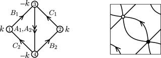
Figure 2: The quiver diagram and the brane tiling for a theory dual to $Q^{1,1,1}/{\bf Z}_{k}$.

The superpotential of the Chern-Simons theory is

$$W=\mathop{\rm tr}\nolimits(\epsilon^{ij}C_{2}B_{1}A_{i}B_{2}C_{1}A_{j}).$$ (95)

When the Chern-Simons levels are $(k,k,-k,-k)$, the corresponding geometry is $Q^{1,1,1}/{\bf Z}_{k}$ where ${\bf Z}_{k}$ is a subgroup of the diagonal $SU(2)$ in $SU(2)_{2}\times SU(2)_{3}$, and break it down to $U(1)_{F}\times U(1)_{B}$. The manifest global symmetry of this theory is

$$SU(2)\times U(1)_{F}\times U(1)_{B}\times U(1)_{R}.$$ (96)

$SU(2)$ is the symmetry acting on $A_{i}$. Note that the action does not have $SU(2)$ symmetries rotating $B_{i}$ and $C_{i}$. We define three generators $F_{i}$ ($i=1,2,3$) of the Cartan part of the flavor symmetry $SU(2)\times U(1)_{F}\times U(1)_{B}$. $F_{2}+F_{3}$ and $F_{2}-F_{3}$ generate $U(1)_{B}$ and $U(1)_{F}$, respectively. The charge assignments are shown in Table 2.

Table 2: Charge assignments of R and flavor symmetries of the theory in Fig. 2 are shown.

	$A_{1}$	$A_{2}$	$B_{1}$	$B_{2}$	$C_{1}$	$C_{2}$
$\Delta$	$1-2h$	$1-2h$	$h$	$h$	$h$	$h$
$F_{1}$	$\frac{1}{2}$	$-\frac{1}{2}$	$0$	$0$	$0$	$0$
$F_{2}$	$0$	$0$	$\frac{1}{2}$	$-\frac{1}{2}$	$0$	$0$
$F_{3}$	$0$	$0$	$0$	$0$	$\frac{1}{2}$	$-\frac{1}{2}$

From only the symmetry of the action and the marginality of the superpotential the R-charges of the chiral fields are not fixed. We have an ambiguity of an unknown parameter $h$. The index does not depend on $h$, and we do not need to determine it.

The $SU(2)$ symmetry of the action guarantees that the index satisfy

$$I(x,z_{1},z_{2},z_{3})=I(x,z_{1}^{-1},z_{3},z_{2}),$$ (97)

and the index is expanded by $SU(2)$ characters $\chi_{s}(z_{1})$. This theory also has ${\bf Z}_{2}$ symmetry which exchanges $B_{i}$ and $C_{i}$, and the index satisfies the relation

$$I(x,z_{1},z_{2},z_{3})=I(x,z_{1},z_{3},z_{2}).$$ (98)

Another relation follows from the charge conjugation symmetry. If we apply the charge conjugation to the theory, all arrows are reversed and the resulting diagram is obtained by rotating the original one by 180 degrees. This exchanges $B_{1}$ and $B_{2}$, and $C_{1}$ and $C_{2}$. This implies the relation

$$I^{(-)}(x,z_{1},z_{2},z_{3})=I^{(+)}(x,z_{1},z_{2}^{-1},z_{3}^{-1}),$$ (99)

and the symmetry of the index,

$$I(x,z_{1},z_{2},z_{3})=I(x,z_{1},z_{2}^{-1},z_{3}^{-1}).$$ (100)

If the flavor symmetry is enhanced to $SU(2)^{3}$ in $k=1$ case, $I(x,z_{i})$ must have a larger symmetry. It should be invariant under Weyl Group of three $SU(2)$, which inverses three $z_{i}$ independently. We also expect the permutation symmetry among $z_{i}$. Let us confirm this symmetry enhancement by computing the index in $k=1$ case.

The neutral part of the index is

$$I^{(0)}(x,z_{i})=1+\chi_{\frac{1}{2}}(z_{1})\left(\frac{z_{2}^{1/2}}{z_{3}^{1/2}}+\frac{z_{3}^{1/2}}{z_{2}^{1/2}}\right)x+\left[\chi_{1}(z_{1})\left(2\frac{z_{2}}{z_{3}}+1+2\frac{z_{3}}{z_{2}}\right)-3\right]x^{2}+\cdots.$$ (101)

There are three contributions to $I^{(+)}$ up to the order of $x^{2}$,

$$I^{(+)}_{(\vbox{\vbox{\offinterlineskip\vbox{\hrule height=0.3pt\hbox{\vrule height=2.72pt,width=0.3pt,depth=0.67998pt\hbox to3.4pt{\hfil}\vrule height=2.72pt,width=0.3pt,depth=0.67998pt} \hrule height=0.3pt}\vspace{-\y@linethick} }},\vbox{\vbox{\offinterlineskip\vbox{\hrule height=0.3pt\hbox{\vrule height=2.72pt,width=0.3pt,depth=0.67998pt\hbox to3.4pt{\hfil}\vrule height=2.72pt,width=0.3pt,depth=0.67998pt} \hrule height=0.3pt}\vspace{-\y@linethick} }},\vbox{\vbox{\offinterlineskip\vbox{\hrule height=0.3pt\hbox{\vrule height=2.72pt,width=0.3pt,depth=0.67998pt\hbox to3.4pt{\hfil}\vrule height=2.72pt,width=0.3pt,depth=0.67998pt} \hrule height=0.3pt}\vspace{-\y@linethick} }},\vbox{\vbox{\offinterlineskip\vbox{\hrule height=0.3pt\hbox{\vrule height=2.72pt,width=0.3pt,depth=0.67998pt\hbox to3.4pt{\hfil}\vrule height=2.72pt,width=0.3pt,depth=0.67998pt} \hrule height=0.3pt}\vspace{-\y@linethick} }})}(x,z_{i}) = \chi_{\frac{1}{2}}(z_{1})z_{2}^{-1/2}z_{3}^{-1/2}x+(\chi_{1}(z_{1})-1)(z_{2}^{-1}+z_{3}^{-1})x^{2}+\cdots,$$

$$I^{(+)}_{(\vbox{\vbox{\offinterlineskip\vbox{\hrule height=0.3pt\hbox{\vrule height=2.72pt,width=0.3pt,depth=0.67998pt\hbox to3.4pt{\hfil}\vrule height=2.72pt,width=0.3pt,depth=0.67998pt\hbox to3.4pt{\hfil}\vrule height=2.72pt,width=0.3pt,depth=0.67998pt} \hrule height=0.3pt}\vspace{-\y@linethick} }},\vbox{\vbox{\offinterlineskip\vbox{\hrule height=0.3pt\hbox{\vrule height=2.72pt,width=0.3pt,depth=0.67998pt\hbox to3.4pt{\hfil}\vrule height=2.72pt,width=0.3pt,depth=0.67998pt\hbox to3.4pt{\hfil}\vrule height=2.72pt,width=0.3pt,depth=0.67998pt} \hrule height=0.3pt}\vspace{-\y@linethick} }},\vbox{\vbox{\offinterlineskip\vbox{\hrule height=0.3pt\hbox{\vrule height=2.72pt,width=0.3pt,depth=0.67998pt\hbox to3.4pt{\hfil}\vrule height=2.72pt,width=0.3pt,depth=0.67998pt\hbox to3.4pt{\hfil}\vrule height=2.72pt,width=0.3pt,depth=0.67998pt} \hrule height=0.3pt}\vspace{-\y@linethick} }},\vbox{\vbox{\offinterlineskip\vbox{\hrule height=0.3pt\hbox{\vrule height=2.72pt,width=0.3pt,depth=0.67998pt\hbox to3.4pt{\hfil}\vrule height=2.72pt,width=0.3pt,depth=0.67998pt\hbox to3.4pt{\hfil}\vrule height=2.72pt,width=0.3pt,depth=0.67998pt} \hrule height=0.3pt}\vspace{-\y@linethick} }})}(x,z_{i}) = \chi_{1}(z_{1})z_{2}^{-1}z_{3}^{-1}x^{2}+\cdots,$$

$$I^{(+)}_{(\vbox{\vbox{\offinterlineskip\vbox{\hrule height=0.3pt\hbox{\vrule height=2.72pt,width=0.3pt,depth=0.67998pt\hbox to3.4pt{\hfil}\vrule height=2.72pt,width=0.3pt,depth=0.67998pt} \hrule height=0.3pt}\vspace{-\y@linethick} \vbox{\hrule height=0.3pt\hbox{\vrule height=2.72pt,width=0.3pt,depth=0.67998pt\hbox to3.4pt{\hfil}\vrule height=2.72pt,width=0.3pt,depth=0.67998pt} \hrule height=0.3pt}\vspace{-\y@linethick} }},\vbox{\vbox{\offinterlineskip\vbox{\hrule height=0.3pt\hbox{\vrule height=2.72pt,width=0.3pt,depth=0.67998pt\hbox to3.4pt{\hfil}\vrule height=2.72pt,width=0.3pt,depth=0.67998pt} \hrule height=0.3pt}\vspace{-\y@linethick} \vbox{\hrule height=0.3pt\hbox{\vrule height=2.72pt,width=0.3pt,depth=0.67998pt\hbox to3.4pt{\hfil}\vrule height=2.72pt,width=0.3pt,depth=0.67998pt} \hrule height=0.3pt}\vspace{-\y@linethick} }},\vbox{\vbox{\offinterlineskip\vbox{\hrule height=0.3pt\hbox{\vrule height=2.72pt,width=0.3pt,depth=0.67998pt\hbox to3.4pt{\hfil}\vrule height=2.72pt,width=0.3pt,depth=0.67998pt} \hrule height=0.3pt}\vspace{-\y@linethick} \vbox{\hrule height=0.3pt\hbox{\vrule height=2.72pt,width=0.3pt,depth=0.67998pt\hbox to3.4pt{\hfil}\vrule height=2.72pt,width=0.3pt,depth=0.67998pt} \hrule height=0.3pt}\vspace{-\y@linethick} }},\vbox{\vbox{\offinterlineskip\vbox{\hrule height=0.3pt\hbox{\vrule height=2.72pt,width=0.3pt,depth=0.67998pt\hbox to3.4pt{\hfil}\vrule height=2.72pt,width=0.3pt,depth=0.67998pt} \hrule height=0.3pt}\vspace{-\y@linethick} \vbox{\hrule height=0.3pt\hbox{\vrule height=2.72pt,width=0.3pt,depth=0.67998pt\hbox to3.4pt{\hfil}\vrule height=2.72pt,width=0.3pt,depth=0.67998pt} \hrule height=0.3pt}\vspace{-\y@linethick} }})}(x,z_{i}) = \chi_{1}(z_{1})z_{2}^{-1}z_{3}^{-1}x^{2}+\cdots.$$ (102)

Summing up these three and the trivial one $I^{(+)}_{(\cdot,\cdot,\cdot,\cdot)}=1$, we obtain

$$I^{(+)}=1+\chi_{\frac{1}{2}}(z_{1})z_{2}^{-1/2}z_{3}^{-1/2}x+\left[(\chi_{1}(z_{1})-1)(z_{2}^{-1}+z_{3}^{-1})+2\chi_{1}(z_{1})z_{2}^{-1}z_{3}^{-1}\right]x^{2}+\cdots.$$ (103)

This satisfies (97) and (98). We obtain $I^{(-)}$ by the relation (100),

$$I^{(-)}=1+\chi_{\frac{1}{2}}(z_{1})z_{2}^{1/2}z_{3}^{1/2}x+\left[(\chi_{1}(z_{1})-1)(z_{2}+z_{3})+2\chi_{1}(z_{1})z_{2}z_{3}\right]x^{2}+\cdots.$$ (104)

As the product of (101), (103), and (104) we obtain the index

$$I(x,z_{i})=1+\chi_{\frac{1}{2}}(z_{1})\chi_{\frac{1}{2}}(z_{2})\chi_{\frac{1}{2}}(z_{3})x+(2\chi_{1}(z_{1})\chi_{1}(z_{2})\chi_{1}(z_{3})-2)x^{2}+\cdots.$$ (105)

This is invariant under the Weyl reflections $z_{2}\rightarrow z_{2}^{-1}$ and $z_{3}\rightarrow z_{3}^{-1}$, and under permutations among $z_{i}$. This is precisely what we expect from the isometry of $Q^{1,1,1}$. The single particle index for (105) is

$$I^{\rm sp}(x,z_{i})=\chi_{\frac{1}{2}}(z_{1})\chi_{\frac{1}{2}}(z_{2})\chi_{\frac{1}{2}}(z_{3})x$$

$$\hskip 20.00003pt+\left(\chi_{1}(z_{1})\chi_{1}(z_{2})\chi_{1}(z_{3})-\chi_{1}(z_{1})-\chi_{1}(z_{2})-\chi_{1}(z_{3})-2\right)x^{2}+\cdots.$$ (106)

We also consider $k=2$ case. Only non-vanishing contribution to $I^{(+)}$ up to the order of $x^{2}$ is

$$I_{(\vbox{\vbox{\offinterlineskip\vbox{\hrule height=0.3pt\hbox{\vrule height=2.72pt,width=0.3pt,depth=0.67998pt\hbox to3.4pt{\hfil}\vrule height=2.72pt,width=0.3pt,depth=0.67998pt} \hrule height=0.3pt}\vspace{-\y@linethick} }},\vbox{\vbox{\offinterlineskip\vbox{\hrule height=0.3pt\hbox{\vrule height=2.72pt,width=0.3pt,depth=0.67998pt\hbox to3.4pt{\hfil}\vrule height=2.72pt,width=0.3pt,depth=0.67998pt} \hrule height=0.3pt}\vspace{-\y@linethick} }},\vbox{\vbox{\offinterlineskip\vbox{\hrule height=0.3pt\hbox{\vrule height=2.72pt,width=0.3pt,depth=0.67998pt\hbox to3.4pt{\hfil}\vrule height=2.72pt,width=0.3pt,depth=0.67998pt} \hrule height=0.3pt}\vspace{-\y@linethick} }},\vbox{\vbox{\offinterlineskip\vbox{\hrule height=0.3pt\hbox{\vrule height=2.72pt,width=0.3pt,depth=0.67998pt\hbox to3.4pt{\hfil}\vrule height=2.72pt,width=0.3pt,depth=0.67998pt} \hrule height=0.3pt}\vspace{-\y@linethick} }})}=x^{2}\frac{\chi_{1}(z_{1})}{z_{2}z_{3}}+\cdots,$$ (107)

and the index $I$ and the corresponding single particle index $I^{\rm sp}$ are

$$I = 1+x\chi_{1}(z_{1})\left(\frac{z_{2}^{1/2}}{z_{3}^{1/2}}+\frac{z_{3}^{1/2}}{z_{2}^{1/2}}\right)$$ (108)

$$+x^{2}\left[\chi_{1}(z_{1})\left(z_{2}z_{3}+\frac{1}{z_{2}z_{3}}+2\frac{z_{2}}{z_{3}}+2\frac{z_{3}}{z_{2}}+1\right)-3\right]\cdots,$$

$$I^{\rm sp} = x\chi_{1}(z_{1})\left(\frac{z_{2}^{1/2}}{z_{3}^{1/2}}+\frac{z_{3}^{1/2}}{z_{2}^{1/2}}\right)$$ (109)

$$+x^{2}\left[\chi_{1}(z_{1})\left(z_{2}z_{3}+\frac{1}{z_{2}z_{3}}+\frac{z_{2}}{z_{3}}+\frac{z_{3}}{z_{2}}\right)-4\right]+\cdots.$$

Because the dual geometry is the orbifold $Q^{1,1,1}/{\bf Z}_{k}$, (109) should be obtained from (106) by the projection associated with $(z_{1},z_{2},z_{3})\rightarrow(z_{1},e^{\pi i}z_{2},e^{\pi i}z_{3})$. We can easily confirm that this is actually the case.

There is another realization of $Q^{1,1,1}$ by a quiver Chern-Simons theory[36]. It is described by the same quiver diagram as the previous one and has the same superpotential, but has different Chern-Simons levels $(k,-k,0,0)$.

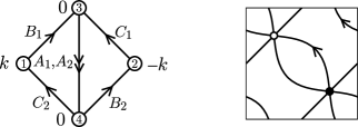
Figure 3: The quiver diagram and the brane tiling for a theory dual to $Q^{1,1,1}/{\bf Z}_{k}$. The Chern-Simons levels are different from Figure 3.

The charge assignments are shown in Table 3.

Table 3: Charge assignments of R and flavor symmetries of the theory in Fig. 3 are shown.

	$A_{1}$	$A_{2}$	$B_{1}$	$B_{2}$	$C_{1}$	$C_{2}$
$\Delta$	$1-2h$	$1-2h$	$h$	$h$	$h$	$h$
$F_{1}$	$\frac{1}{2}$	$-\frac{1}{2}$	$0$	$0$	$0$	$0$
$F_{2}$	$0$	$0$	$\frac{1}{2}$	$0$	$-\frac{1}{2}$	$0$
$F_{3}$	$0$	$0$	$0$	$\frac{1}{2}$	$0$	$-\frac{1}{2}$

Due to the different Chern-Simons levels, the $U(1)_{B}$ charge of this theory rotates fields in a different way from the previous one. We define $F_{2}$ and $F_{3}$ so that $F_{2}+F_{3}$ again generates the baryonic symmetry. The manifest flavor symmetry of the action guarantees

$$I(x,z_{1},z_{2},z_{3})=I(x,z_{1}^{-1},z_{2},z_{3}),$$ (110)

and the charge conjugation gives the relation

$$I(x,z_{1},z_{2},z_{3})=I(x,z_{1},z_{3}^{-1},z_{2}^{-1}).$$ (111)

We computed the index for $k=1,2$, and we obtain the same results for $I^{(0)},I^{(+)}$ and $I^{(-)}$ as the previous theory for $Q^{1,1,1}$.

8 Example 3: $Q^{2,2,2}$

The homogeneous Sasaki-Einstein space $Q^{2,2,2}$ is defined as the orbifold $Q^{1,1,1}/{\bf Z}_{2}$. The generator of the orbifold group ${\bf Z}_{2}$ is $e^{\pi i(R+2j_{3})}$. The isometry group of $Q^{2,2,2}$ is the same as $Q^{1,1,1}$.

Dual Chern-Simons theories for $Q^{2,2,2}$ are proposed in [36]. We first consider the theory shown in Fig. 4.

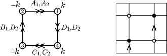
Figure 4: The quiver diagram and the brane tiling for a theory dual to $Q^{2,2,2}/{\bf Z}_{k}$.

This theory has the superpotential

$$W=\epsilon^{ik}\epsilon^{jl}\mathop{\rm tr}\nolimits(A_{i}B_{j}C_{k}D_{l}).$$ (112)

The manifest global symmetry of this theory is

$$SU(2)\times SU(2)\times U(1)_{B}\times U(1)_{R}.$$ (113)

The first $SU(2)$ acts on $A_{i}$ and $C_{i}$, and the second on $B_{i}$ and $D_{i}$. Let $F_{1}$ and $F_{2}$ be the generators of two $SU(2)$ groups, and $F_{3}$ be the generator of the baryonic $U(1)$. The conformal dimensions of fields and the charge assignments are shown in Table 4.

Table 4: The R-charge assignment and charge assignments of the theory in Fig. 4 are shown.

	$A_{1}$	$A_{2}$	$B_{1}$	$B_{2}$	$C_{1}$	$C_{2}$	$D_{1}$	$D_{2}$
$\Delta$	$h$	$h$	$1-h$	$1-h$	$h$	$h$	$1-h$	$1-h$
$F_{1}$	$\frac{1}{2}$	$-\frac{1}{2}$	$0$	$0$	$\frac{1}{2}$	$-\frac{1}{2}$	$0$	$0$
$F_{2}$	$0$	$0$	$\frac{1}{2}$	$-\frac{1}{2}$	$0$	$0$	$\frac{1}{2}$	$-\frac{1}{2}$
$F_{3}$	$\frac{1}{2}$	$\frac{1}{2}$	$0$	$0$	$-\frac{1}{2}$	$-\frac{1}{2}$	$0$	$0$

The Weyl group of the flavor symmetry guarantees the relations

$$I(x,z_{1},z_{2},z_{3})=I(x,z_{1}^{-1},z_{2},z_{3})=I(x,z_{1},z_{2}^{-1},z_{3}).$$ (114)

We also have

$$I(x,z_{1},z_{2},z_{3})=I(x,z_{1},z_{2},z_{3}^{-1})$$ (115)

from the charge conjugation symmetry. These generate the Weyl group of $SU(2)^{3}$, but it is non-trivial whether the index respects the permutation symmetry among $z_{i}$ when $k=1$.

Let us compute the index for $k=1$. The neutral part is

$$I^{(0)}=1+x^{2}\left[(\chi_{1}(z_{1})-1)(\chi_{1}(z_{2})-1)-4\right]+\cdots,$$ (116)

and the only monopole contributions to $I^{(+)}$ up to $x^{2}$ is

$$I^{(+)}_{(\vbox{\vbox{\offinterlineskip\vbox{\hrule height=0.3pt\hbox{\vrule height=2.72pt,width=0.3pt,depth=0.67998pt\hbox to3.4pt{\hfil}\vrule height=2.72pt,width=0.3pt,depth=0.67998pt} \hrule height=0.3pt}\vspace{-\y@linethick} }},\vbox{\vbox{\offinterlineskip\vbox{\hrule height=0.3pt\hbox{\vrule height=2.72pt,width=0.3pt,depth=0.67998pt\hbox to3.4pt{\hfil}\vrule height=2.72pt,width=0.3pt,depth=0.67998pt} \hrule height=0.3pt}\vspace{-\y@linethick} }},\vbox{\vbox{\offinterlineskip\vbox{\hrule height=0.3pt\hbox{\vrule height=2.72pt,width=0.3pt,depth=0.67998pt\hbox to3.4pt{\hfil}\vrule height=2.72pt,width=0.3pt,depth=0.67998pt} \hrule height=0.3pt}\vspace{-\y@linethick} }},\vbox{\vbox{\offinterlineskip\vbox{\hrule height=0.3pt\hbox{\vrule height=2.72pt,width=0.3pt,depth=0.67998pt\hbox to3.4pt{\hfil}\vrule height=2.72pt,width=0.3pt,depth=0.67998pt} \hrule height=0.3pt}\vspace{-\y@linethick} }})}=x^{2}\left[\chi_{1}(z_{1})\chi_{1}(z_{2})-1\right]z_{3}+\cdots.$$ (117)

The whole index $I$ and the corresponding single particle index $I^{\rm sp}$ are

$$I = 1+\left[\chi_{1}(z_{1})\chi_{1}(z_{2})\chi_{1}(z_{3})-\chi_{1}(z_{1})-\chi_{1}(z_{2})-\chi_{1}(z_{3})-2\right]x^{2}+\cdots,$$ (118)

$$I^{\rm sp} = \left(\chi_{1}(z_{1})\chi_{1}(z_{2})\chi_{1}(z_{3})-\chi_{1}(z_{1})-\chi_{1}(z_{2})-\chi_{1}(z_{3})-2\right)x^{2}+\cdots.$$ (119)

These have expected permutation symmetry. Because $Q^{2,2,2}$ is the ${\bf Z}_{2}$ orbifold of $Q^{1,1,1}$, (119) should be related to (106) by the orbifold projection. The orbifold group ${\bf Z}_{2}$ is generated by $e^{\pi i(R+2j_{3})}$. On BPS operators saturating the BPS bound (2) this parity is equal to $e^{\pi i(\Delta+j_{3})}$, and flips the sign of $x$. (119) is what is obtained from (106) by the projection associated with this ${\bf Z}_{2}$ flip $x\rightarrow-x$.

There is another theory proposed as a dual to $Q^{2,2,2}$[36]. (Fig. 5)

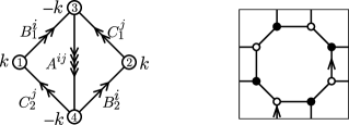
Figure 5: The quiver diagram and the brane tiling for a dual theory to $Q^{2,2,2}/{\bf Z}_{k}$ are shown.

The superpotential of this theory is

$$W=\mathop{\rm tr}\nolimits(\epsilon_{ij}\epsilon_{kl}A^{ik}B_{1}^{j}C_{2}^{l}-\epsilon_{ij}\epsilon_{kl}A^{ik}B_{2}^{j}C_{1}^{l}),$$ (120)

and the manifest global symmetry of the action is

$$SU(2)_{1}\times SU(2)_{2}\times U(1)_{B}\times U(1)_{R}.$$ (121)

We define $F_{1}$, $F_{2}$, and $F_{3}$ as generators of the $SU(2)_{1}$ Cartan, the $SU(2)_{2}$ Cartan, and $U(1)_{B}$, respectively.

Table 5: The R and flavor charge assignments of the theory in Fig. 5 are shown.

	$A^{ij}$	$B_{1}^{i}$	$B_{2}^{i}$	$C_{1}^{j}$	$C_{2}^{j}$
$\Delta$	$2-2h$	$h$	$h$
$F_{1}$	$\pm\frac{1}{2}$	$\pm\frac{1}{2}$	$\pm\frac{1}{2}$	$0$	$0$
$F_{2}$	$\pm\frac{1}{2}$	$0$	$0$	$\pm\frac{1}{2}$	$\pm\frac{1}{2}$
$F_{3}$	$0$	$\frac{1}{2}$	$-\frac{1}{2}$	$\frac{1}{2}$	$-\frac{1}{2}$

The manifest $SU(2)_{1}\times SU(2)_{2}$ symmetry guarantees the relations

$$I(x,z_{1},z_{2},z_{3})=I(x,z_{1}^{-1},z_{2},z_{3})=I(x,z_{1},z_{2}^{-1},z_{3}),$$ (122)

and the charge conjugation guarantees

$$I(x,z_{1},z_{2},z_{3})=I(x,z_{1},z_{2},z_{3}^{-1}).$$ (123)

The neutral part is the same as (116), and the only non-vanishing contribution to $I^{(+)}$ up to the order of $x^{2}$ is

$$I_{(\vbox{\vbox{\offinterlineskip\vbox{\hrule height=0.3pt\hbox{\vrule height=2.72pt,width=0.3pt,depth=0.67998pt\hbox to3.4pt{\hfil}\vrule height=2.72pt,width=0.3pt,depth=0.67998pt} \hrule height=0.3pt}\vspace{-\y@linethick} }},\vbox{\vbox{\offinterlineskip\vbox{\hrule height=0.3pt\hbox{\vrule height=2.72pt,width=0.3pt,depth=0.67998pt\hbox to3.4pt{\hfil}\vrule height=2.72pt,width=0.3pt,depth=0.67998pt} \hrule height=0.3pt}\vspace{-\y@linethick} }},\vbox{\vbox{\offinterlineskip\vbox{\hrule height=0.3pt\hbox{\vrule height=2.72pt,width=0.3pt,depth=0.67998pt\hbox to3.4pt{\hfil}\vrule height=2.72pt,width=0.3pt,depth=0.67998pt} \hrule height=0.3pt}\vspace{-\y@linethick} }},\vbox{\vbox{\offinterlineskip\vbox{\hrule height=0.3pt\hbox{\vrule height=2.72pt,width=0.3pt,depth=0.67998pt\hbox to3.4pt{\hfil}\vrule height=2.72pt,width=0.3pt,depth=0.67998pt} \hrule height=0.3pt}\vspace{-\y@linethick} }})}=x^{2}[\chi_{1}(z_{1})\chi_{1}(z_{2})-1]z_{3}^{-1}.$$ (124)

The indices $I$ and $I^{\rm sp}$ are identical to (118) and (119), respectively.

9 Example 4: $M^{1,1,1}$

$M^{1,1,1}$, which is also often called $M^{3,2}$, is the coset

$$\frac{SU(3)\times SU(2)\times U(1)}{SU(2)\times U(1)\times U(1)},$$ (125)

and has the isometry

$$SU(3)\times SU(2)\times U(1).$$ (126)

The $U(1)$ factor is identified with the $U(1)_{R}$ symmetry.

A quiver Chern-Simons theory dual to $M^{1,1,1}$ is proposed in [32, 33]. It is $U(N)^{3}$ Chern-Simons theory shown in Fig. 6.

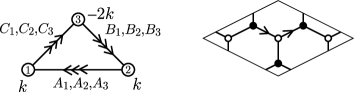
Figure 6: The quiver diagram for a theory dual to $M^{1,1,1}/{\bf Z}_{k}$.

The superpotential is

$$W=\epsilon^{ijk}\mathop{\rm tr}\nolimits(A_{i}B_{j}C_{k}).$$ (127)

The manifest global symmetry of this theory is

$$SU(3)\times U(1)_{B}\times U(1)_{R},$$ (128)

where $SU(3)$ rotates $A_{i}$, $B_{i}$, and $C_{i}$ simultaneously. $U(1)_{B}$ is the baryonic symmetry acting on $B_{i}$ and $C_{i}$ with opposite charges. We introduce $F_{1}$ and $F_{2}$ as $SU(3)$ Cartan generators, and $F_{3}$ as $U(1)_{B}$ charge. The charge assignments are shown in Table 6.

Table 6: Charge assignments of R and flavor symmetries for the $M^{1,1,1}$ theory are shown.

	$A_{1}$	$A_{2}$	$A_{3}$	$B_{1}$	$B_{2}$	$B_{3}$	$C_{1}$	$C_{2}$	$C_{3}$
$\Delta$	$2-2h$	$2-2h$	$2-2h$	$h$	$h$	$h$	$h$	$h$	$h$
$F_{1}$	$1$	$-1$	$0$	$1$	$-1$	$0$	$1$	$-1$	$0$
$F_{2}$	$0$	$1$	$-1$	$0$	$1$	$-1$	$0$	$1$	$-1$
$F_{3}$	$0$	$0$	$0$	$\frac{1}{2}$	$\frac{1}{2}$	$\frac{1}{2}$	$-\frac{1}{2}$	$-\frac{1}{2}$	$-\frac{1}{2}$

Due to the manifest $SU(3)$ symmetry, the index is invariant under the $SU(3)$ Weyl group generated by the relations

$$I(x,z_{1},z_{2},z_{3})=I(x,z_{2}^{-1},z_{1}^{-1},z_{3})=I(x,z_{1},z_{1}z_{2}^{-1},z_{3}).$$ (129)

The charge conjugation gives the relation

$$I^{(-)}(x,z_{1},z_{2},z_{3})=I^{(+)}(x,z_{1},z_{2},z_{3}^{-1}),$$ (130)

between $I^{(+)}$ and $I^{(-)}$, and the symmetry of the index

$$I(x,z_{1},z_{2},z_{3})=I(x,z_{1},z_{2},z_{3}^{-1}).$$ (131)

Disappointingly, the Weyl group of the full flavor symmetry $SU(3)\times SU(2)$ is exhausted by the relations generated by (129) and (131), and thus computation of the index and simple symmetry analysis does not give extra information about the symmetry enhancement from $U(1)_{B}$ to $SU(2)$. We give some results in $k=1$ case just for reference. The neutral part of the index up to $x^{2}$ is

$$I^{(0)} = 1+\left(z_{1}^{3}+\frac{z_{2}^{3}}{z_{1}^{3}}+\frac{1}{z_{2}^{3}}-3\right)x^{2}+\cdots$$ (132)

$$= 1+(\chi^{SU(3)}_{(3,0)}(z_{1},z_{2})-\chi^{SU(3)}_{(1,1)}(z_{1},z_{2})-2)x^{2}+\cdots,$$

where $\chi^{SU(3)}_{(a_{1},a_{2})}$ is the $SU(3)$ character of the representation with Dynkin label $(a_{1},a_{2})$. Our definition here is such that for the fundamental and the anti-fundamental representations,

$$\chi^{SU(3)}_{(1,0)}(z_{1},z_{2})=z_{1}+\frac{z_{2}}{z_{1}}+\frac{1}{z_{2}},\quad\chi^{SU(3)}_{(0,1)}(z_{1},z_{2})=\frac{1}{z_{1}}+\frac{z_{1}}{z_{2}}+z_{2}.$$ (133)

The only monopole contribution to $I^{(+)}$ up to order $x^{2}$ is

$$I_{(\vbox{\vbox{\offinterlineskip\vbox{\hrule height=0.3pt\hbox{\vrule height=2.72pt,width=0.3pt,depth=0.67998pt\hbox to3.4pt{\hfil}\vrule height=2.72pt,width=0.3pt,depth=0.67998pt} \hrule height=0.3pt}\vspace{-\y@linethick} }},\vbox{\vbox{\offinterlineskip\vbox{\hrule height=0.3pt\hbox{\vrule height=2.72pt,width=0.3pt,depth=0.67998pt\hbox to3.4pt{\hfil}\vrule height=2.72pt,width=0.3pt,depth=0.67998pt} \hrule height=0.3pt}\vspace{-\y@linethick} }},\vbox{\vbox{\offinterlineskip\vbox{\hrule height=0.3pt\hbox{\vrule height=2.72pt,width=0.3pt,depth=0.67998pt\hbox to3.4pt{\hfil}\vrule height=2.72pt,width=0.3pt,depth=0.67998pt} \hrule height=0.3pt}\vspace{-\y@linethick} }})}^{(+)} = \left(z_{1}+\frac{z_{2}}{z_{1}}+\frac{1}{z_{2}}\right)\left(z_{1}^{2}+\frac{z_{2}^{2}}{z_{1}^{2}}+\frac{1}{z_{2}^{2}}\right)z_{3}x^{2}+\cdots$$ (134)

$$= (\chi_{(3,0)}^{SU(3)}(z_{1},z_{2})-1)z_{3}x^{2}+\cdots.$$

The index $I$ and the corresponding $I^{\rm sp}$ are

$$I = 1+[(\chi_{(3,0)}^{SU(3)}(z_{1},z_{2})-1)\chi_{1}(z_{3})-\chi_{(1,1)}^{SU(3)}(z_{1},z_{2})-1]x^{2}+\cdots,$$ (135)

$$I^{\rm sp} = [(\chi_{(3,0)}^{SU(3)}(z_{1},z_{2})-1)\chi_{1}(z_{3})-\chi_{(1,1)}^{SU(3)}(z_{1},z_{2})-1]x^{2}+\cdots.$$ (136)

10 Adding flavors

Let us extend the formula obtained in previous sections to the theories with flavors belonging to fundamental and anti-fundamental representations[41, 42, 43, 44].

The contribution of chiral multiplets in (anti-)fundamental representations to the letter index is obtained from (20) by setting $\rho^{\prime}=0$ ($\rho=0$). The contribution of fundamental representations is

$$f^{\bf N}_{\rm chiral}(e^{ia},x,z_{i}) = \sum_{\Phi_{A0}}\sum_{\rho\in{\bf N}_{A}}\frac{x^{|\rho(m)|}}{1-x^{2}}$$ (137)

$$\hskip 20.00003pt\left(e^{i\rho(a)}z_{i}^{F_{i}(\Phi)}x^{\Delta(\Phi)}-e^{-i\rho(a)}z_{i}^{-F_{i}(\Phi)}x^{2-\Delta(\Phi)}\right)$$

$$= \sum_{\Phi_{A0}}\left(\lambda_{A,+1}\frac{z_{i}^{F_{i}(\Phi)}x^{\Delta(\Phi)}}{1-x^{2}}-\lambda_{A,-1}\frac{z_{i}^{-F_{i}(\Phi)}x^{2-\Delta(\Phi)}}{1-x^{2}}\right),$$

where $\Phi_{A0}$ represents chiral multiplets belonging to the $U(N)_{A}$ fundamental representation ${\bf N}_{A}$. The contribution of anti-fundamental representations is

$$f^{\overline{\bf N}}_{\rm chiral}(e^{ia},x,z_{i})=\sum_{\Phi_{0B}}\left(\lambda_{B,-1}\frac{z_{i}^{F_{i}(\Phi)}x^{\Delta(\Phi)}}{1-x^{2}}-\lambda_{B,+1}\frac{z_{i}^{-F_{i}(\Phi)}x^{2-\Delta(\Phi)}}{1-x^{2}}\right).$$ (138)

$\Phi_{0B}$ represents chiral multiplets belonging to the $U(N)_{B}$ anti-fundamental representation $\overline{\bf N}_{B}$

(137) and (138) depend on $a^{(0)}$ through $\lambda_{A,m}$ defined in (39), and we include this contribution to the definition of $f^{\prime}$. There is no change in the definition of $f^{(\pm)}$. Only bi-fundamental fields contribute to $f^{(\pm)}$.

Let us define $V_{A}$ and $W_{A}$ by

$$f_{\rm chiral}^{\bf N}+f_{\rm chiral}^{\overline{\bf N}}=\sum_{A=1}^{n_{G}}(V_{A}\lambda_{A,-1}+\lambda_{A,1}W_{A}).$$ (139)

The neutral part of index $I^{(0)}$ is defined by Gaussian integral including (139) in the exponent,

$$I^{(0)} = \int d\lambda\exp\sum_{n=1}^{\infty}\frac{1}{n}\Bigg{(}-\sum_{A,B}\lambda_{A,n}M_{A,B}(\cdot^{n})\lambda_{B,-n}$$ (140)

$$\hskip 90.00014pt+\sum_{A}V_{A}(\cdot^{n})\lambda_{A,-n}+\sum_{A}\lambda_{A,n}W_{A}(\cdot^{n})\Bigg{)}$$

$$= \prod_{n=1}^{\infty}\frac{1}{\det M_{A,B}(\cdot^{n})}\exp\left(\frac{1}{n}\sum_{A,B}V_{A}(\cdot^{n})(M^{-1}(\cdot^{n}))_{A,B}W_{B}(\cdot^{n})\right)$$

Compared to (42), (140) has the extra exponential factor. This contributes to the single particle index by

$$\sum_{A,B}V_{A}(x,z_{i})(M^{-1}(x,z_{i}))_{A,B}W_{B}(x,z_{i}).$$ (141)

The introduction of flavors changes the zero-point contributions to the energy, the flavor charges, and the gauge charges. The extra contributions are

$$\epsilon_{0}^{\rm fund} = \frac{1}{2}\sum_{\Phi_{A0},\Phi_{0A}}\sum_{\rho\in{\bf N}_{A}}|\rho(m)|(1-\Delta(\Phi)),$$ (142)

$$q_{0i}^{\rm fund} = -\frac{1}{2}\sum_{\Phi_{A0},\Phi_{0A}}\sum_{\rho\in{\bf N}_{A}}|\rho(m)|F_{i}(\Phi),$$ (143)

$$b_{0}^{\rm fund}(a) = -\frac{1}{2}\sum_{\Phi_{A0}}\sum_{\rho\in{\bf N}_{A}}|\rho(m)|\rho(a)+\frac{1}{2}\sum_{\Phi_{0A}}\sum_{\rho\in{\bf N}_{A}}|\rho(m)|\rho(a).$$ (144)

For vector-like theories, $b_{0}(a)$ identically vanishes. These do not depend on $a^{(0)}$, and are added to the definition of $\epsilon^{(\pm)}$, $q_{0i}^{(\pm)}$, and $b_{0}^{(\pm)}(a)$.

11 Example 5: $N^{0,1,0}$

As an example of a theory with flavors, let us consider a flavored ABJM model, which is proposed as a dual theory to $N^{0,1,0}$[42].

$N^{0,1,0}$ is the homogeneous manifold defined as the coset

$$SU(3)/U(1),$$ (145)

and its isometry is

$$SU(3)\times SU(2).$$ (146)

This manifold is hyper-Kähler and respects ${\cal N}=3$ supersymmetry. The $SU(2)$ factor in (146) is the R-symmetry rotating three supercharges. We use only two of them for the localization.

The theory dual to $N^{0,1,0}$ is defined by adding one vector-like flavor $(q,\widetilde{q})$ to the ABJM model, which has gauge group $U(N)_{1}\times U(N)_{2}$. $q$ and $\widetilde{q}$ belong to the fundamental and the anti-fundamental representations of $U(N)_{1}$. The quiver diagram of this theory is shown in Fig. 7.

Figure 7: The quiver diagram of a flavored ABJM model dual to $N^{0,1,0}$ is shown. The box represents a global $U(1)$ symmetry.

The superpotential is

$$W=\mathop{\rm tr}\nolimits[(\epsilon^{ij}A_{i}B_{j}+q\widetilde{q})^{2}-(\epsilon^{ij}B_{i}A_{j})^{2}]$$ (147)

The introduction of the flavor breaks the ${\cal N}=6$ supersymmetry of the ABJM model to ${\cal N}=3$. Due to the non-abelian R-symmetry $SU(2)_{R}$ the R-charges are protected from quantum corrections and all chiral multiplets have the canonical R-charge $1/2$. The manifest global symmetry of the theory is

$$SU(2)\times U(1)_{B}\times SU(2)_{R}.$$ (148)

$SU(2)$ rotates $A_{i}$ and $B_{i}$ as doublets. The dual geometry of this model is $N^{0,1,0}/{\bf Z}_{k}$. We would like to confirm that the flavor symmetry $SU(2)\times U(1)_{B}$ is enhanced to $SU(3)$ in $k=1$ case. Let $F_{1}$ and $F_{2}$ be the generators of $SU(2)$ Cartan and the baryonic symmetry, respectively. The charge assignments are shown in Table 7.

Table 7: The charge assignments of R and flavor symmetries in the $N^{0,1,0}$ theory are shown.

	$q$	$\widetilde{q}$	$A_{1}$	$A_{2}$	$B_{1}$	$B_{2}$
$\Delta$	$\frac{1}{2}$	$\frac{1}{2}$	$\frac{1}{2}$	$\frac{1}{2}$	$\frac{1}{2}$	$\frac{1}{2}$
$F_{1}$	$0$	$0$	$\frac{1}{2}$	$-\frac{1}{2}$	$\frac{1}{2}$	$-\frac{1}{2}$
$F_{2}$	$1$	$-1$	$1$	$1$	$-1$	$-1$

The manifest $SU(2)$ symmetry guarantees the relation

$$I(x,z_{1},z_{2})=I(x,z_{1}^{-1},z_{2}).$$ (149)

From the charge conjugation symmetry, we obtain the relation

$$I^{(-)}(x,z_{1},z_{2})=I^{(+)}(x,z_{1},z_{2}^{-1}).$$ (150)

The neutral part $I^{(0)}$ is

$$I^{(0)}=1+x(\chi_{1}(z_{1})+2)+x^{2}(2\chi_{2}(z_{1})+2\chi_{1}(z_{1})+3)+\cdots.$$ (151)

The non-trivial contributions to the positive part $I^{(+)}$ up to $x^{2}$ are

$$I^{(+)}_{(\vbox{\vbox{\offinterlineskip\vbox{\hrule height=0.3pt\hbox{\vrule height=2.72pt,width=0.3pt,depth=0.67998pt\hbox to3.4pt{\hfil}\vrule height=2.72pt,width=0.3pt,depth=0.67998pt} \hrule height=0.3pt}\vspace{-\y@linethick} }},\vbox{\vbox{\offinterlineskip\vbox{\hrule height=0.3pt\hbox{\vrule height=2.72pt,width=0.3pt,depth=0.67998pt\hbox to3.4pt{\hfil}\vrule height=2.72pt,width=0.3pt,depth=0.67998pt} \hrule height=0.3pt}\vspace{-\y@linethick} }})} = \left[x\chi_{\frac{1}{2}}(z_{1})+x^{2}\chi_{\frac{3}{2}}(z_{1})+\cdots\right]z_{2},$$ (152)

$$I^{(+)}_{(\vbox{\vbox{\offinterlineskip\vbox{\hrule height=0.3pt\hbox{\vrule height=2.72pt,width=0.3pt,depth=0.67998pt\hbox to3.4pt{\hfil}\vrule height=2.72pt,width=0.3pt,depth=0.67998pt\hbox to3.4pt{\hfil}\vrule height=2.72pt,width=0.3pt,depth=0.67998pt} \hrule height=0.3pt}\vspace{-\y@linethick} }},\vbox{\vbox{\offinterlineskip\vbox{\hrule height=0.3pt\hbox{\vrule height=2.72pt,width=0.3pt,depth=0.67998pt\hbox to3.4pt{\hfil}\vrule height=2.72pt,width=0.3pt,depth=0.67998pt\hbox to3.4pt{\hfil}\vrule height=2.72pt,width=0.3pt,depth=0.67998pt} \hrule height=0.3pt}\vspace{-\y@linethick} }})} = x^{2}\chi_{1}(z_{1})z_{2}^{2}+\cdots,$$ (153)

$$I^{(+)}_{(\vbox{\vbox{\offinterlineskip\vbox{\hrule height=0.3pt\hbox{\vrule height=2.72pt,width=0.3pt,depth=0.67998pt\hbox to3.4pt{\hfil}\vrule height=2.72pt,width=0.3pt,depth=0.67998pt} \hrule height=0.3pt}\vspace{-\y@linethick} \vbox{\hrule height=0.3pt\hbox{\vrule height=2.72pt,width=0.3pt,depth=0.67998pt\hbox to3.4pt{\hfil}\vrule height=2.72pt,width=0.3pt,depth=0.67998pt} \hrule height=0.3pt}\vspace{-\y@linethick} }},\vbox{\vbox{\offinterlineskip\vbox{\hrule height=0.3pt\hbox{\vrule height=2.72pt,width=0.3pt,depth=0.67998pt\hbox to3.4pt{\hfil}\vrule height=2.72pt,width=0.3pt,depth=0.67998pt} \hrule height=0.3pt}\vspace{-\y@linethick} \vbox{\hrule height=0.3pt\hbox{\vrule height=2.72pt,width=0.3pt,depth=0.67998pt\hbox to3.4pt{\hfil}\vrule height=2.72pt,width=0.3pt,depth=0.67998pt} \hrule height=0.3pt}\vspace{-\y@linethick} }})} = x^{2}\chi_{1}(z_{1})z_{2}^{2}+\cdots.$$ (154)

Combining these contributions, we obtain the complete index $I$ and the corresponding single-particle index $I^{\rm sp}$,

$$I = 1+x(\chi^{SU(3)}_{(1,1)}(z_{1},z_{2})+1)+x^{2}(2\chi^{SU(3)}_{(2,2)}(z_{1},z_{2})+\chi^{SU(3)}_{(1,1)}(z_{1},z_{2})+1)+\cdots,$$ (155)

$$I^{\rm sp} = x(\chi^{SU(3)}_{(1,1)}(z_{1},z_{2})+1)+x^{2}(\chi^{SU(3)}_{(2,2)}(z_{1},z_{2})-\chi^{SU(3)}_{(1,1)}(z_{1},z_{2})-1)+\cdots,$$ (156)

where $\chi^{SU(3)}_{(a_{1},a_{2})}$ is the $SU(3)$ character for the representation with Dynkin label $(a_{1},a_{2})$. We here define $\chi_{(a_{1},a_{2})}^{SU(3)}$ in a different way from (133). The characters for fundamental and the anti-fundamental representations are

$$\chi_{(1,0)}^{SU(3)}(z_{1},z_{2})=z_{2}^{1/3}\chi_{\frac{1}{2}}(z_{1})+z_{2}^{-2/3},\quad\chi_{(0,1)}^{SU(3)}(z_{1},z_{2})=z_{2}^{-1/3}\chi_{\frac{1}{2}}(z_{1})+z_{2}^{2/3}.$$ (157)

The form of the index strongly suggest the enhancement of the global symmetry to $SU(3)$.

12 Conclusions

We derived a formula of the superconformal index for ${\cal N}=2$ superconformal large $N$ quiver Chern-Simons theories. In the case of vector-like models, we confirmed the factorization of the index into the neutral, the positive, and the negative parts. For chiral theories, the factorization was confirmed only in the sector of diagonal monopole operators. We did not take account of non-diagonal monopole operators on the assumption that they are non-BPS and do not contribute to the index. In this paper, we have not proved this on the gauge theory side. It would be important to analyze the contribution of non-diagonal operators systematically for understanding of the relation between non-diagonal monopole operators and wrapped M2-branes in AdS₄/CFT₃.

We applied the formula to some Chern-Simons theories which have been proposed as dual theories to M-theory in homogeneous spaces, $V^{5,2}$, $Q^{1,1,1}$, $Q^{2,2,2}$, $M^{1,1,1}$, and $N^{0,1,0}$. The actions of these theories do not have full global symmetries which exist on the gravity side as isometries of the internal spaces. We computed the index for each theory up to the order of $x^{2}$, and confirmed that it is invariant under the Weyl group of the full symmetry expected from $AdS/CFT$ if we include the contribution of diagonal monopole operators. In other wards, the index is a linear combination of characters of the full symmetry. This result strongly suggests that the global symmetry of the Chern-Simons theory is enhanced to the full symmetry non-perturbatively.

We emphasize that we only confirm the invariance of the index under the Weyl group, and it does not guarantee the enhancement of the continuous symmetry. To obtain more convincing evidences of the symmetry enhancement, we need to compare the index to the result of Kaluza-Klein analysis on the gravity side. Such an analysis is important especially for inhomogeneous Sasaki-Einstein spaces in which we have no symmetry enhancement in general.

References

[1]
J. M. Maldacena,
“The large N limit of superconformal field theories and supergravity,”
Adv. Theor. Math. Phys. 2, 231 (1998)
[Int. J. Theor. Phys. 38, 1113 (1999)]
[arXiv:hep-th/9711200].
[2]
J. Kinney, J. M. Maldacena, S. Minwalla and S. Raju,
“An index for 4 dimensional super conformal theories,”
Commun. Math. Phys. 275, 209 (2007)
[arXiv:hep-th/0510251].
[3]
C. Romelsberger,
“Counting chiral primaries in N = 1, d=4 superconformal field theories,”
Nucl. Phys. B 747, 329 (2006)
[arXiv:hep-th/0510060].
[4]
Y. Nakayama,
“Index for orbifold quiver gauge theories,”
Phys. Lett. B 636, 132 (2006)
[arXiv:hep-th/0512280].
[5]
Y. Nakayama,
“Index for supergravity on AdS(5) x T**(1,1) and conifold gauge theory,”
Nucl. Phys. B 755, 295 (2006)
[arXiv:hep-th/0602284].
[6]
S. Benvenuti, B. Feng, A. Hanany and Y. H. He,
“Counting BPS operators in gauge theories: Quivers, syzygies and
plethystics,”
JHEP 0711, 050 (2007)
[arXiv:hep-th/0608050].
[7]
C. Romelsberger,
“Calculating the Superconformal Index and Seiberg Duality,”
arXiv:0707.3702 [hep-th].
[8]
F. A. Dolan and H. Osborn,
“Applications of the Superconformal Index for Protected Operators and
q-Hypergeometric Identities to N=1 Dual Theories,”
Nucl. Phys. B 818, 137 (2009)
[arXiv:0801.4947 [hep-th]].
[9]
V. P. Spiridonov and G. S. Vartanov,
“Superconformal indices for theories with multiple duals,”
Nucl. Phys. B 824, 192 (2010)
[arXiv:0811.1909 [hep-th]].
[10]
A. Gadde, L. Rastelli, S. S. Razamat and W. Yan,
“On the Superconformal Index of N=1 IR Fixed Points: A Holographic Check,”
arXiv:1011.5278 [hep-th].
[11]
O. Aharony, O. Bergman, D. L. Jafferis and J. Maldacena,
“N=6 superconformal Chern-Simons-matter theories, M2-branes and their
gravity duals,”
JHEP 0810, 091 (2008)
[arXiv:0806.1218 [hep-th]].
[12]
J. Bhattacharya and S. Minwalla,
“Superconformal Indices for Chern Simons Theories,”
JHEP 0901, 014 (2009)
[arXiv:0806.3251 [hep-th]].
[13]
S. Kim,
“The complete superconformal index for N=6 Chern-Simons theory,”
Nucl. Phys. B 821, 241 (2009)
[arXiv:0903.4172 [hep-th]].
[14]
J. Choi, S. Lee and J. Song,
“Superconformal Indices for Orbifold Chern-Simons Theories,”
JHEP 0903, 099 (2009)
[arXiv:0811.2855 [hep-th]].
[15]
Y. Imamura and S. Yokoyama,
“A Monopole Index for N=4 Chern-Simons Theories,”
Nucl. Phys. B 827, 183 (2010)
[arXiv:0908.0988 [hep-th]].
[16]
S. Kim and J. Park,
“Probing AdS4/CFT3 proposals beyond chiral rings,”
JHEP 1008, 069 (2010)
[arXiv:1003.4343 [hep-th]].
[17]
Y. Imamura and S. Yokoyama,
“Index for three dimensional superconformal field theories with general
R-charge assignments,”
arXiv:1101.0557 [hep-th].
[18]
D. Fabbri, P. Fre’, L. Gualtieri, C. Reina, A. Tomasiello, A. Zaffaroni and A. Zampa,
“3D superconformal theories from Sasakian seven-manifolds: New nontrivial
evidences for AdS(4)/CFT(3),”
Nucl. Phys. B 577, 547 (2000)
[arXiv:hep-th/9907219].
[19]
Y. Imamura and S. Yokoyama,
“N=4 Chern-Simons theories and wrapped M-branes in their gravity duals,”
Prog. Theor. Phys. 121, 915 (2009)
[arXiv:0812.1331 [hep-th]].
[20]
N. Benishti, D. Rodriguez-Gomez and J. Sparks,
“Baryonic symmetries and M5 branes in the AdS4/CFT3 correspondence,”
JHEP 1007, 024 (2010)
[arXiv:1004.2045 [hep-th]].
[21]
P. Goddard, J. Nuyts and D. I. Olive,
“Gauge Theories And Magnetic Charge,”
Nucl. Phys. B 125, 1 (1977).
[22]
V. A. Novikov, M. A. Shifman, A. I. Vainshtein and V. I. Zakharov,
“Exact Gell-Mann-Low Function Of Supersymmetric Yang-Mills Theories From
Instanton Calculus,”
Nucl. Phys. B 229, 381 (1983).
[23]
V. A. Novikov, M. A. Shifman, A. I. Vainshtein and V. I. Zakharov,
“Supersymmetric instanton calculus: Gauge theories with matter,”
Nucl. Phys. B 260, 157 (1985)
[Yad. Fiz. 42, 1499 (1985)].
[24]
V. A. Novikov, M. A. Shifman, A. I. Vainshtein and V. I. Zakharov,
“Beta Function In Supersymmetric Gauge Theories: Instantons Versus
Traditional Approach,”
Phys. Lett. B 166, 329 (1986)
[Sov. J. Nucl. Phys. 43, 294 (1986)]
[Yad. Fiz. 43, 459 (1986)].
[25]
D. Martelli and J. Sparks,
“AdS4/CFT3 duals from M2-branes at hypersurface singularities and their
deformations,”
JHEP 0912, 017 (2009)
[arXiv:0909.2036 [hep-th]].
[26]
A. Hanany and D. Vegh,
“Quivers, tilings, branes and rhombi,”
JHEP 0710, 029 (2007)
[arXiv:hep-th/0511063].
[27]
A. Hanany and K. D. Kennaway,
“Dimer models and toric diagrams,”
arXiv:hep-th/0503149.
[28]
S. Franco, A. Hanany, K. D. Kennaway, D. Vegh and B. Wecht,
“Brane Dimers and Quiver Gauge Theories,”
JHEP 0601, 096 (2006)
[arXiv:hep-th/0504110].
[29]
S. Franco, A. Hanany, D. Martelli, J. Sparks, D. Vegh and B. Wecht,
“Gauge theories from toric geometry and brane tilings,”
JHEP 0601, 128 (2006)
[arXiv:hep-th/0505211].
[30]
K. D. Kennaway,
“Brane Tilings,”
Int. J. Mod. Phys. A 22, 2977 (2007)
[arXiv:0706.1660 [hep-th]].
[31]
M. Yamazaki,
“Brane Tilings and Their Applications,”
Fortsch. Phys. 56, 555 (2008)
[arXiv:0803.4474 [hep-th]].
[32]
D. Martelli and J. Sparks,
“Moduli spaces of Chern-Simons quiver gauge theories and AdS(4)/CFT(3),”
Phys. Rev. D 78, 126005 (2008)
[arXiv:0808.0912 [hep-th]].
[33]
A. Hanany and A. Zaffaroni,
“Tilings, Chern-Simons Theories and M2 Branes,”
JHEP 0810, 111 (2008)
[arXiv:0808.1244 [hep-th]].
[34]
K. Ueda and M. Yamazaki,
“Toric Calabi-Yau four-folds dual to Chern-Simons-matter theories,”
JHEP 0812, 045 (2008)
[arXiv:0808.3768 [hep-th]].
[35]
Y. Imamura and K. Kimura,
“Quiver Chern-Simons theories and crystals,”
JHEP 0810, 114 (2008)
[arXiv:0808.4155 [hep-th]].
[36]
S. Franco, A. Hanany, J. Park and D. Rodriguez-Gomez,
“Towards M2-brane Theories for Generic Toric Singularities,”
JHEP 0812, 110 (2008)
[arXiv:0809.3237 [hep-th]].
[37]
S. Franco, I. R. Klebanov and D. Rodriguez-Gomez,
“M2-branes on Orbifolds of the Cone over Q1,1,1,”
JHEP 0908, 033 (2009)
[arXiv:0903.3231 [hep-th]].
[38]
S. Lee,
“Superconformal field theories from crystal lattices,”
Phys. Rev. D 75, 101901 (2007)
[arXiv:hep-th/0610204].
[39]
S. Lee, S. Lee and J. Park,
“Toric AdS(4)/CFT(3) duals and M-theory crystals,”
JHEP 0705, 004 (2007)
[arXiv:hep-th/0702120].
[40]
S. Kim, S. Lee, S. Lee and J. Park,
“Abelian Gauge Theory on M2-brane and Toric Duality,”
Nucl. Phys. B 797, 340 (2008)
[arXiv:0705.3540 [hep-th]].
[41]
M. Ammon, J. Erdmenger, R. Meyer, A. O’Bannon and T. Wrase,
“Adding Flavor to AdS4/CFT3,”
JHEP 0911, 125 (2009)
[arXiv:0909.3845 [hep-th]].
[42]
D. Gaiotto and D. L. Jafferis,
“Notes on adding D6 branes wrapping RP3 in AdS4 x CP3,”
arXiv:0903.2175 [hep-th].
[43]
F. Benini, C. Closset and S. Cremonesi,
“Chiral flavors and M2-branes at toric CY4 singularities,”
JHEP 1002, 036 (2010)
[arXiv:0911.4127 [hep-th]].
[44]
D. L. Jafferis,
“Quantum corrections to N=2 Chern-Simons theories with flavor and their AdS4
duals,”
arXiv:0911.4324 [hep-th].