Extended time-travelling objects in Misner space

Abstract

Misner space is a two-dimensional (2D) locally-flat spacetime which elegantly demonstrates the emergence of closed timelike curves from causally well-behaved initial conditions. Here we explore the motion of rigid extended objects in this time-machine spacetime. This kind of 2D time-travel is found to be risky due to inevitable self-collisions (i.e. collisions of the object with itself). However, in a straightforward four-dimensional generalization of Misner space (a physically more relevant spacetime obviously), we find a wide range of safe time-travel orbits free of any self-collisions.

I Introduction

About 40 years ago, Misner misner_space introduced an amazing vacuum solution of the Einstein equations, known as the Misner space. This is a two-dimensional (2D) spacetime which describes the formation of closed timelike curves (CTCs) from causally well-behaved initial conditions. The solution evolves from an initial spacelike hypersurface $T=const<0$, in a causally well-behaved manner, up to a ”moment” (actually a null hypersurface) denoted $T=0$. Subsequently, the spacetime extends smoothly to the domain $T>0$, in which all points rest on CTCs. It thus nicely demonstrates the phenomenon of smooth formation of CTCs from causally well-behaved initial conditions. This solution may straightforwardly be extended to any $d>2$ dimensions.

Quite remarkably, Misner space is actually flat. It may be obtained from the Minkowski spacetime by a certain cut-and-paste operation, in a manner resembling the construction of a cone by folding the flat Euclidean plane.

One of the outstanding open questions in spacetime physics is that of CTCs formation: Do the laws of nature permit the creation of CTCs from physically and causally well-behaved initial conditions? As it stands, Misner space falls short of providing a compelling ”realistic” physical example —mainly due to its topologically-nontrivial ($S^{1}\times\mathbb{R}^{d-1}$) character (which apparently makes it incompatible with the asymptotics of our realistic spacetime). Several other interesting examples of time-machine spacetimes were introduced previously Classic_models , but all of them suffer from some severe physical problems. Nevertheless, it was recently demonstrated that a certain non-flat generalization of Misner space (based on the ”pseudo-Schwarzschild” metric rather than Minkowski) may be used to construct a more feasible time-machine model Amos_Time_Machine_2007 : Namely, an asymptotically-flat and topologically-trivial four-dimensional (4D) spacetime which satisfies all the energy conditions, and which smoothly develops CTCs at a certain stage.

Beside these constructional issues, one may be concerned about other unusual physical phenomena which may take place in a time-machine spacetime. In particular, several authors stability investigated the stability of classical and quantum fields in certain time-machine spacetimes. There are obvious indications for linear instabilities of various kinds in the neighborhood of the Chronology horizon stability . It is still unclear, however, what will be the outcome of these instabilities in the full nonlinear context.

In this work we introduce an additional probe for the nature of physical processes on a time-machine background: We consider the motion of physical objects of finite size, and examine whether such objects can penetrate (and traverse) the region of CTCs, without being destroyed or damaged by self-collisions. For simplicity we shall consider here the Misner space (in two or more dimensions). Since this spacetime is flat, no tidal forces will act on the object, which may therefore be considered as rigid. Yet the nontrivial identifications may result in self collisions—e.g. a ”head-tail” collision of the object’s two edges.

A brief look reveals that such self-collisions certainly occur for some orbits, but the more interesting question is whether it is possible to choose orbits which avoid these collisions. We shall show that it is fairly easy to avoid self-collisions up to $T=0$. However, in the 2D case, collisions are found to be inevitable once the object has crossed into $T>0$.

Nevertheless, we shall demonstrate here that for any $d>2$ a collision-free motion is possible, throughout the region of CTCs, for a wide, nonzero-measure, range of orbits. This includes the case of most obvious physical relevance, namely that of a three-dimensional rigid object moving in 4D Misner space.

We note that the motion of extended objects has been analyzed previously by several authors, mostly during the 1990s, in the context of the ”billiard-ball” problem Thorne billiard ; Mensky and novikov . To the best of our knowledge, however, these investigations were restricted to the wormhole-based time-machine spacetime Morris . We are not aware of extensions of the ”billiard-ball” analyses to the Misner-space background—or to any other background spacetime which similarly satisfies the energy conditions . Note also, that Misner space is especially convenient due to its flatness, which implies vanishing tidal forces and hence conceptually simplifies the notion of ”rigid extended object”.

In section II we describe the basic structure of Misner space and analyze its geodesics. Section III is devoted to analyzing an extended object in a 2D Misner space, whereas in section IV we extend Misner space to three dimensions and analyze the object’s motion in this extended model. Section V treats the four-dimensional case, and in section VI we briefly discuss our results.

Throughout the paper we use relativistic units in which $c=1$.

II Misner space

Misner space misner_space is a 2D spacetime with the metric

$$ds^{2}=-2dTd\psi-Td\psi^{2},$$ (1)

where $-\infty<T<\infty$ but the coordinate $\psi$ is periodic, that is, each $\psi$ is identified with $\psi+\psi_{0}$ for a certain parameter $\psi_{0}>0$. Since $det(g)=-1$ the metric (1) is perfectly regular everywhere and in particularly at $T=0$.

The curves $T=const$ are all closed due to the periodicity of $\psi$. Whereas the $T<0$ curves are spacelike, the $T>0$ curves are timelike. It then follows that all points at $T>0$ rest on CTCs but those at $T<0$ do not. The curve $T=0$ is null, and it serves as the chronology horizon (i.e. the hypersurface separating the causal and non-causal parts of spacetime).

Any hypersurface $T=const\equiv T_{0}<0$ is spacelike and can be chosen as an initial hypersurface over which initial data (for both geometry and physical fields) may be specified. The hypersurface $T=0$ is a Cauchy horizon for any such initial hypersurface $T=T_{0}<0$. The Cauchy evolution of the latter unambiguously yields the portion $T_{0}<T<0$ of Misner space. Assuming that the evolution beyond the Cauchy horizon proceeds in an analytic manner, we recover the region $T>0$ as well, and CTCs appear. Hence Misner space satisfactorily describes the formation of CTCs from rather conventional (though topologically non-trivial) initial conditions.

The metric (1) is flat, so in a local sense it is equivalent to 2D Minkowski. However, in a global sense it is drastically different from Minkowski due to the identification of $\psi$. The universal covering of Misner space is obtained by unfolding the coordinate $\psi$, namely by setting -$\infty<\psi<\infty$. In this covering space the portions $T<0$ and $T>0$ correspond to regions I and II of Minkowski, respectively, as shown in Fig. 1. There are infinite number of Misner copies in these two regions of Minkowski.

We begin by presenting the Misner process — the procedure which transforms the Minkowski spacetime into Misner. To this end we introduce an intermediate, Rindler-like, coordinate $z$ which will be useful in later analysis. Following the Misner process we derive the geodesics in the Misner coordinates and also discuss their relation to the Rindler-like coordinate $z$.

II.1 Coordinate transformation

We start with the 2D Minkowski metric

$$ds^{2}=-dt^{2}+dx^{2}.$$ (2)

Misner’s covering space occupies only the portion $x<t$ of Minkowski, namely the gray regions I and II in Fig. 1. We first elaborate on region I. We consider the coordinate transformation

$$x = -2\sqrt{-T}sinh\left(\frac{z}{2}\right),$$

$$t = -2\sqrt{-T}cosh\left(\frac{z}{2}\right),$$ (3)

where $T<0$ and $-\infty<z<\infty$. This leads to the metric

$$ds^{2}=\frac{dT^{2}}{T}-Tdz^{2}.$$ (4)

We now introduce the coordinate $\psi$ by

$$\psi=z-ln|T|.$$ (5)

Transforming the line element (4) from $z$ to $\psi$, one obtains Misner’s metric (1).

The analytic extension of the metric (1) from $T<0$ (region I) to $T>0$ (region II) is straightforward. However, we note that the transformation (3) only applies to region I. In order to directly transform region II from ($t,x$) to ($T,z$), we must modify the transformation into

$$x = 2\sqrt{T}cosh\left(\frac{z}{2}\right),$$

$$t = 2\sqrt{T}sinh\left(\frac{z}{2}\right).$$ (6)

It will result in the metric (4) as before. [The transformation (5) defining $\psi$ applies to $T>0$ without any modification, and yields the metric (1) in region II as well.]

Note that the lines $T=const$ are spacelike in region I and timelike in region II, and the lines $z=const$ are timelike in I and spacelike in II. On the other hand, the lines $\psi=const$ are everywhere null.

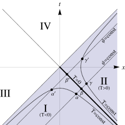
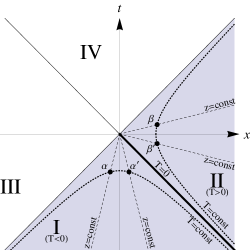
Figure 1: Misner space and its universal covering presented in Minkowski coordinates ($t,x$). In both figures (a,b), the universal covering (the portion $t<x$, which corresponds to $-\infty<\psi<\infty$) is the gray region, consisting of the two Minkowski quadrants I and II. In the Misner space (compactified $\psi$), the two diagonal lines denoted ”$\psi=const$” in Fig.1 are identified. Alternatively, Misner’s identification may be implemented by identifying two $z=const$ lines. This is demonstrated in Fig. 1, which displays a pair of such identified $z=const$ lines in each of the quadrants I, II. In both figures identification points are marked by the same Greek letter.

So far we have constructed Misner’s metric (1) on the (topologically-trivial) ”half-Minkowski” manifold, namely the union of regions I and II in Fig. 1. In the next stage, we choose a parameter $\psi_{0}>0$ and fold the $\psi$ coordinate by identifying $\psi$ with $\psi+\psi_{0}$ (at the same $T$). The coordinate $T$ still takes the entire range $-\infty<T<\infty$. A pair of such identified constant-$\psi$ lines, embedded in the half-Minkowski covering space, is shown in Fig. 1. On these two lines we marked identified points by the same Greek letter. These identified pairs of points all lie on constant-$T$ lines.

It will be useful to note at this stage that identifying the $\psi$ coordinate at the same $T$ value is equivalent to the identification of the $z$ coordinate at the same $T$ [see Eq. (5)]. Lines of constant $z$ are presented in Fig. 1, along with the constant-$T$ lines. Again, we marked identified points by the same Greek letter.

Altogether the transformation from Minkowski to Misner is:

$$t=Te^{\frac{\psi}{2}}-e^{-\frac{\psi}{2}},$$

$$x=Te^{\frac{\psi}{2}}+e^{-\frac{\psi}{2}},$$ (7)

and the inverse transformation is:

$$\psi = -2\ln\left(\frac{x-t}{2}\right),$$ (8)

$$T = \frac{x^{2}-t^{2}}{4}.$$ (9)

These relations hold at both regions I and II.

As was mentioned above, Misner’s identification can be manifested by identifying two lines of constant $z$ (at the same $T$, and with $z$ values separated by $\psi_{0}$). The velocity $dx/dt$ is fixed along each such line of constant $z$ [cf. Eqs. (3) or (6)], therefore the relative velocity between a pair of identified $z=const$ lines is well defined. A straightforward calculation reveals that this relative velocity is $u=Tanh(\psi_{0}/2)$. Thus, Misner’s “folding” process may be viewed as identification under the action of a boost with velocity $u$.

Let (p,q) be a pair of points in the half-Minkowski covering space, and let (p’,q’) be their images under a certain (generic) boost. Since in 2D Minkowski spacetime any two boosts are commutative, it immediately follows that p’ and q’ are identified (under Misner’s folding) if and only if p and q are identified. It thus follows that the 2D Misner space inherits the boost invariance of Minkowski.

II.2 Geodesics

Our main interest in this work is the motion of a rigid object in Misner space. To simplify the analysis, we shall employ the above mentioned boost symmetry and choose a Lorentz frame in which the object is at rest [namely, $x(t)=const$]. We start here by analyzing the properties of a single such geodesic.

It is convenient to express the geodesics using their corresponding function $T(\psi)$ . A single static geodesic satisfies (in the covering space) $x=const\equiv x_{0}$, which by virtue of Eq. (7) yields

$$T(\psi)=-e^{-\psi}+x_{0}e^{-\frac{\psi}{2}}.$$ (10)

Consider the propagation of such an $x=x_{0}$ geodesic from some $T<0$ toward $T=0$. The relation (10) makes it clear that there are two different classes of such geodesics: Those with $x_{0}<0$ only approach $T=0$ at $\psi\to\infty$. On the other hand, those with $x_{0}>0$ will all reach $T=0$ at a finite $\psi$, and continue their journey in the region $T>0$ . Since our primary objective is the motion of extended objects into the region of CTCs ($T>0$), throughout the rest of the paper we shall restrict our attention to the second class, namely the $x_{0}>0$ geodesics.

Consider now the behavior of those $x_{0}>0$ geodesics at $T>0$. For each of these geodesics the function $T(\psi)$ will reach its maximum at its intersection point with $t=0$. This behavior is demonstrated in Fig. 2, which displays two different $x=x_{0}>0$ geodesics, as well as the line $t=0$. This property can be easily deduced by finding the $(T,\psi)$ coordinates at the maximum point of the relation (10), and using Eq. (7) in order to obtain the corresponding $t$ value.

These static geodesics exhibit a simple symmetry when displayed in the $(T,z)$ coordinates. From Eq. (6) we observe that in the $T>0$ region, the relation $x=x_{0}$ yields

$$T(z)=\left(\frac{x_{0}}{2cosh(z/2)}\right)^{2}.$$ (11)

This function is symmetric about $z=0$, hence the maximum of $T$ is attained at $z=0$. This is illustrated in Fig. 2, which displays a single $x=x_{0}$ geodesic and the line $t=0$ in $(T,z)$ coordinates. From Eq. (6) it is also clear that $t=0$ coincides with $z=0$, demonstrating again that the geodesics $x=x_{0}$ reach their maximal $T$ value at a point where $t$ vanishes.

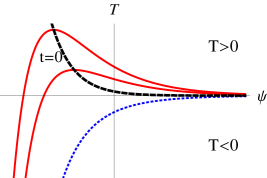
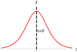
Figure 2: Constant-$x$ geodesics plotted in Misner coordinates ($T,\psi$) and in ($T,z$) coordinates. The dashed black curve represents the $t=0$ line, which in fact coincides with $z=0$. Fig. 2 shows three geodesics: The dotted (blue) curve is an $x_{0}<0$ geodesic. The two solid (red) curves represent $x_{0}>0$ geodesics. These geodesics attain their maximal $T$ values at their intersection with $t=0$. Fig. 2 demonstrates the symmetry of a single ($x_{0}>0$) geodesic around $z=0$.

III Rod motion: the two dimensional case

Consider now a rigid extended object, a ”rod”, which moves freely in 2D Misner space. The rod may be considered as a one-parameter family of rod’s points. Presumably no external forces are present, and since Misner space is flat, the tidal force vanishes as well, so all rod’s points are expected to move on geodesics (as long as self-collisions have not occurred). The rod’s motion in spacetime is thus described by a congruence of timelike geodesics. Rigidity implies that these geodesics are all parallel (in $x$-$t$ coordinates). However, the identification of $\psi$ may lead to a collision of two rod’s points. Furthermore, at $T>0$ a rod point may even collide with itself (owing to the presence of CTCs). Our main objective is to investigate whether such collisions may be prevented.

Exploiting the boost-invariance of Misner space, we choose a Lorentz frame in which the rod is at rest (in the corresponding Minkowskian universal-covering space), so all geodesics in the rod’s congruence satisfy $x=const\equiv x_{0}$. Each rod’s point is thus characterized by its $x_{0}$ value.

The rod presumably starts its journey at the pre-CTCs region $T<0$, and moves towards the CTCs region $T>0$. We shall first consider the journey toward the chronology horizon, namely the domain $T<0$.

We denote the rod’s two edges by $x_{0}=a_{1}$ and $x_{0}=a_{2}$, assuming $0<a_{1}<a_{2}$. Figs. 3(a-c) display the orbits of the two edge geodesics (in the universal covering space) by dashed (red) lines, in $t$-$x$, $T$-$\psi$, and $T$-$z$ coordinates, using Eqs. (10) and (11). The rod thus occupies the region between the two red lines, marked by gray in Figs. 3 and 3. Evidently, a necessary and sufficient condition for a safe journey up to the chronology horizon will be that at any slice $T=constant\leq 0$, the $\psi$-difference between the two edges will be $<\psi_{0}$.

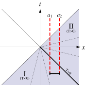
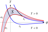
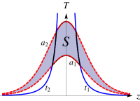
Figure 3: A plot of the rod’s two edge geodesics $x=a_{1,2}$, embedded in the universal covering space. These geodesics are represented by dashed (red) lines — in Minkowski coordinates ($t,x$), in Misner coordinates ($T,\psi$), and in ($T,z$) coordinates, in Figs. 3(a,b,c) respectively. In Fig. 3(a) the short horizontal bold solid (black) line represents the rod, and the two vertical lines are the edge geodesics. In Figs. 3(b,c) the two solid (blue) curves represent curves of constant $t$. In the 2D case, the spacetime region occupied by the rod is the entire gray strip. In the $d\geq 3$ case (with $v\neq 0$, as discussed below), at a given $y=const$ hypersurface the rod occupies the domain $S_{y}$, namely the quadrangle-like region denoted ”S”.

The function $T(\psi)$ of Eq. (10) is monotonic throughout the region $T\leq 0$ and can thus be inverted:

$$\psi(T)=2\ln 2-2\ln[x_{0}+(x_{0}^{2}-4T)^{1/2}].$$ (12)

At constant $T$, the $\psi$-difference between the two edges will be

$$\Delta\psi(T)\equiv|\psi_{2}(T)-\psi_{1}(T)|=2\ln\left(\frac{a_{2}+\sqrt{a_{2}^{2}-4T}}{a_{1}+\sqrt{a_{1}^{2}-4T}}\right).$$ (13)

A collision-free motion will occur if $\Delta\psi(T)<\psi_{0}$ for any $T\leq 0$. Since the right-hand side of Eq. (13) is a monotonically increasing function of $T$, it will reach its maximum (in the domain $T\leq 0$ presently under consideration) at $T=0$. This determines the criterion for a collision-free motion of the rod up to the chronology horizon: $\psi_{0}>2\ln(a_{2}/a_{1})$. This criterion may be reformulated as a condition on $a_{1}$:

$$a_{1}>\frac{L_{x}}{e^{\psi_{0}/2}-1},$$ (14)

where $L_{x}\equiv a_{2}-a_{1}$ is the rod’s length.

We turn now to consider the rod’s motion in the CTCs region $T>0$. As is evident from Eq. (10), the $x_{0}>0$ geodesics reach a (positive) maximal value of $T$, then $T(\psi)$ decreases monotonically until it vanishes as $\psi\to\infty$. This behavior is demonstrated by the two red lines in Fig. 3. We denote this (geodesic-dependent) maximal $T$ value by $T_{max}$. Any constant-$T$ line in the range $0<T<T_{max}$ intersects the geodesic twice, at two different $\psi$ values. For a given geodesic, we denote the $\psi$-difference between these two intersection points by $\delta\psi(T)$. This $\delta\psi(T)$ diverges at the limit $T\to 0_{+}$. A self-collision occurs whenever $\delta\psi(T)=n\psi_{0}$, where hereafter $n$ denotes a nonvanishing integer. Thus, regardless of the value of $\psi_{0}$, there will be an infinite sequence of such self-collisions as $T\to 0_{+}$. This means that any timelike geodesic will hit itself an infinite number of times immediately after crossing $T=0$.

We conclude, that within the framework of 2D Misner space, once a point particle crosses the chronology horizon it will inevitably hit itself. It is obvious that a finite-length rod will be subject to such self-collisions too.

However, our physical spacetime is four-dimensional. Can these extra dimensions save the object from this inevitable fate of self-collisions? The rest of this paper will be devoted to addressing this question. We shall show that by adding one dimension (or more) to the Misner space, the way is opened for a collision-free journey of rigid objects. We shall first demonstrate this in three dimensions, and then address the straightforward extension to four (or more) dimensions.

IV The three-dimensional case

We shall consider now a two-dimensional rigid extended object moving in a three-dimensional spacetime with the flat metric

$$ds^{2}=-2dTd\psi-Td\psi^{2}+dy^{2},$$ (15)

which is the straightforward extension of the 2D Misner metric (1) to three dimensions. As before, $\psi$ is periodic with a period $\psi_{0}$, and $-\infty<T,y<\infty$. Using Eq. (7) again to transform ($T,\psi$) into ($t,x$), one recovers the standard three-dimensional Minkowski line element in the Cartesian coordinates ($t,x,y$).

As was mentioned above, Misner’s identification in the $t$-$x$ (or $T$-$\psi$) plane may be associated to a boost (with relative velocity $u$) in the $x$ direction. Now, in $d>2$ Minkowski spacetime two boosts commute if and only if they are co-directed. By a straightforward extension of the discussion at the end of Sec. II.1 we observe that $d>2$ Misner space is invariant to boosts in the $x$ direction, but not to boosts in any other direction.

Similar to the two-dimensional case, we assume that all object’s points (OPs) move along geodesics. In the Minkowski coordinates these are just straight lines. The object’s rigid motion in spacetime is described by a congruence of parallel timelike geodesics, all sharing the same velocity vector. As before, we use the boost invariance in the $t-x$ plane to pick a Lorentz frame in which the object’s velocity has vanishing $x$ component. We assume, however, that the object does have a nonvanishing velocity $v>0$ in the $y$ direction (otherwise, the previous analysis would still hold at each $y$ separately, and self-collisions would be inevitable at $T>0$). The OPs thus move along the geodesics

$$x(t)=x_{0}\,,\,\,\,y(t)=y_{0}+vt,$$ (16)

where the constants of motion $x_{0},y_{0}$ characterize the object’s individual points. For simplicity we shall consider here a rectangular object described by

$$a_{1}\leq x_{0}\leq a_{2}\,,\,\,\,b_{1}\leq y_{0}\leq b_{2}$$ (17)

with $a_{1}>0$ . The object’s dimensions (in the chosen Lorentz frame) are $\ell^{x}=a_{2}-a_{1}$, $\ell^{y}=b_{2}-b_{1}$. The proper dimensions (as measured in the object’s local rest frame) are $L^{x}=\ell^{x}$ and $L^{y}=\gamma\ell^{y}$, where $\gamma=1/\sqrt{1-v^{2}}$.

A collision occurs when two distinct events (p,q) on the object’s congruence satisfy

$$T_{p}=T_{q},\,\,\,\psi_{p}=\psi_{q}+n\psi_{0},\,\,\,y_{p}=y_{q}.$$ (18)

(These two events either belong to two different object’s geodesics, or to the same geodesic but at different proper times.)

We shall analyze the possibility to avoid self collisions — first at $T\leq 0$, and then at $T>0$.

IV.1 $T\leq 0$

It is easy to see that Eq. (14) remains a sufficient condition for collision-avoidance at $T\leq 0$: First, any collision in 3D must involve, in particular, a collision in the two-dimensional subspace ($T,\psi$) [as manifested by the first two equalities in (18)]. Also the relation (16) for $x(t)$ is the same as it was in the 2D case. Thus, the analysis of the previous section still implies that if Eq. (14) is satisfied, collisions in the ($T,\psi$) subspace will be avoided at $T\leq 0$.

IV.2 $T>0$

Let us denote by S_y the intersection of the object’s congruence (a three-parameter set) with some $y=const$ slice. S_y is a two-parameter set which may be parametrized by ($x_{0},y_{0}$). It occupies a nonzero-measure portion of the $y=const$ hypersurface. We may use ($T,\psi$) as coordinates for this hypersurface—and hence also for its subset S_y. Fig. 3 displays a certain $y=const$ hypersurface and its corresponding subset S_y, which is the quadrangle-like domain denoted ”S”. The association of an OP ($x_{0},y_{0}$) with the corresponding ($T,\psi$) coordinates (for a specific $y$) is done by Eqs. (8,9) — along with Eq. (16), which now reads $x=x_{0}$ and $t=(y-y_{0})/v$. The boundary of S_y thus consists of the two lines $x=a_{1,2}$ and the two lines $t=t_{1,2}$, where $t_{1,2}\equiv(y-b_{1,2})/v$. From Eq. (7), each of these boundary lines corresponds to a curve in the ($T,\psi$) plane, given by either $T=x_{1,2}\,e^{-\psi/2}-e^{-\psi}$ or $T=t_{1,2}\,e^{-\psi/2}+e^{-\psi}$.

For later convenience we define $\Delta t\equiv t_{1}-t_{2}$ and $t_{cen}\equiv(t_{1}+t_{2})/2$, such that $t_{1,2}=t_{cen}\pm\Delta t/2$. Note that $\Delta t=\ell^{y}/v$ is a constant of motion. On the other hand $t_{cen}$ grows linearly with $y$: $t_{cen}(y)=-(b_{1}+b_{2})/2v+y/v$. This will allow us to replace the variable $y$ by $t_{cen}$ in the analysis below.

For any line $T=const$ which intersects S_y, we define $\Delta\psi_{y}(T)$ to be the span of $\psi$ along the intersection of this line with S_y. More precisely, $\Delta\psi_{y}(T)$ is the $\psi$-difference between the two (furthest ) intersection points of the line $T=const$ with the boundary of S_y. We further define $\Delta\psi_{max}(y)\equiv\displaystyle\max_{T>0}\Delta\psi_{y}(T)$. It now immediately follows from Eq. (18) that a collision may occur at a given $y$ only if $\Delta\psi_{max}(y)\geq\psi_{0}$. That is, a collision-free motion is guaranteed if $\Delta\psi_{max}(y)<\psi_{0}$ for all $y$. This raises the issue of whether $\Delta\psi_{max}(y)$ is bounded (as a function of $y$) or not.

It will be easier to explore the dependence of $\Delta\psi_{max}$ on $t_{cen}$ than on $y$. We thus define

$$\Delta\Psi\equiv\max_{t_{cen}}\Delta\psi_{max}(t_{cen}).$$ (19)

If this maximum exists (i.e. it is finite), then the condition for collision-free motion will be simply $\psi_{0}>\Delta\Psi$.

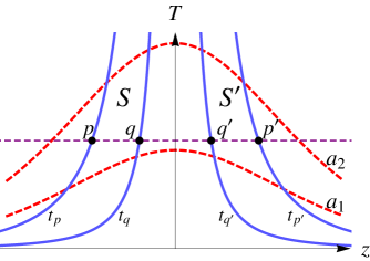
Figure 4: The reflection symmetry of the geodesics and constant-$t$ lines around the $z=0$ line, illustrated in ($T,z$) coordinates. The dashed (red) curves represent the geodesics of the rod’s two edges, $x=a_{1,2}$. The four solid (blue) curves represent curves of constant $t$. S and S’ are two symmetric S_y regions, corresponding to two different $y=const$ slices with the same $|t_{cen}|$.

We shall now employ the reflection symmetry of the problem with respect to the $z$ coordinate to show that it is sufficient to take the maximum of $\Delta\psi_{max}(t_{cen})$ in the range $t_{cen}<0$. To this end all we need to show is that the function $\Delta\psi_{max}(t_{cen})$ is symmetric about $t_{cen}=0$. This symmetry is illustrated in Fig. 4, which displays (in $T$-$z$ coordinates) two different, symmetric, S_y regions, one (denoted S) for which $t_{cen}=-t_{0}$ and the other one (denoted S’) for which $t_{cen}=t_{0}$, for some $t_{0}>0$. The horizontal dashed (purple) line denotes a certain $T=const$ line. The figure also shows the four $t=const$ lines which border these two S_y regions—as well as their four intersection points with the $T=const$ line, denoted by p, q, q’ and p’. Correspondingly we denote the four $t$ values by $t_{p}$, $t_{q}$, $t_{q^{\prime}}$, and $t_{p^{\prime}}$ respectively. Since $|t_{cen}|$ is the same for S and S’ and $\Delta t$ is fixed, one can easily verify that $t_{p^{\prime}}=-t_{p}$ and $t_{q^{\prime}}=-t_{q}$. Consider now the pair of points p and p’. They have a common $T$ but opposite $t$ values ($t_{p^{\prime}}=-t_{p}$). From Eq. (6) it follows that these two points also have opposite $z$ values, $z_{p^{\prime}}=-z_{p}$. The same argument obviously applies to the other pair of points q, q’, and we obtain $z_{q^{\prime}}=-z_{q}$. Defining $\Delta_{z}=z_{q}-z_{p}$ and $\Delta_{z}^{\prime}=z_{p^{\prime}}-z_{q^{\prime}}$, we find that $\Delta_{z}^{\prime}=\Delta_{z}$. However, from Eq. (5) it is obvious that for any pair of points on a given $T=const$ line, the differences in $\psi$ and in $z$ are the same. Therefore, $\Delta\psi_{y}(T)$ (defined above) is the same for S and S’. Since this argument applies to any $T=const$ line , we find that $\Delta\psi_{max}$ is also the same for these two symmetric S_y regions, which completes our argument. We therefore conclude that

$$\Delta\Psi=\max_{t_{cen}\leq 0}\Delta\psi_{max}(t_{cen}).$$ (20)

Next, for any S_y we define $\Delta\tilde{\psi}_{\max}$ to be the maximal $\psi$-difference between all points in S_y. Obviously, for any $T$ (and any given S_y), $\Delta\tilde{\psi}_{\max}\geq\Delta\psi_{y}(T)$, therefore $\Delta\tilde{\psi}_{\max}\geq\Delta\psi_{max}$. As is obvious from the layout of S_y in Fig. 3, $\Delta\tilde{\psi}_{\max}$ is nothing but the $\psi$-difference between the two “corners” $(x=a_{1},t=t_{1})$ and $(x=a_{2},t=t_{2})$ of S_y, and from Eq. (8) it immediately follows that

$$\Delta\tilde{\psi}_{\max}=2\ln\frac{a_{2}-t_{2}}{a_{1}-t_{1}}=2\ln\frac{a_{2}+\Delta t/2-t_{cen}}{a_{1}-\Delta t/2-t_{cen}}.$$ (21)

We now define, in analogy with Eq. (20) above,

$$\Delta\tilde{\Psi}=\max_{t_{cen}\leq 0}\Delta\tilde{\psi}_{\max}(t_{cen}).$$ (22)

Obviously, $\Delta\tilde{\Psi}\geq\Delta\Psi$, hence finiteness of $\Delta\tilde{\Psi}$ will guarantee a finite $\Delta\Psi$—and will ensure collision-free motion for any $\psi_{0}>\Delta\tilde{\Psi}$.

The maximum in Eq. (22) is easily calculated. Notice that $\Delta\tilde{\psi}_{\max}$ is a monotonically-increasing function of $t_{cen}$, therefore the maximum is attained at $t_{cen}=0$:

$$\Delta\tilde{\Psi}=\Delta\tilde{\psi}_{\max}(t_{cen}=0)=2\ln\frac{a_{2}+\Delta t/2}{a_{1}-\Delta t/2}.$$ (23)

Clearly, this parameter is well-defined only if $a_{1}>\Delta t/2$, which we shall assume.

As mentioned above, a sufficient condition for a collision-free motion is $\psi_{0}>\Delta\tilde{\Psi}$. It will be useful to re-express this last inequality as a condition on $a_{1}$, once $\psi_{0}$ is given. Setting $a_{2}=a_{1}+L_{x}$ one obtains the condition

$$a_{1}>\frac{L^{x}+\Delta t}{e^{\psi_{0}/2}-1}+\frac{\Delta t}{2}.$$ (24)

Note that this inequality automatically ensures that $a_{1}>\Delta t/2$ (which was assumed above).

This condition on $a_{1}$ was designed so as to avoid collisions throughout the region $T>0$. However, it is definitely stronger than the inequality (14) which ensured collision-free motion at $T\leq 0$. We therefore conclude that the constraint (24) is a sufficient condition for avoiding collisions throughout the entire Misner space. Stated in other words: Given the spacetime’s identification parameter $\psi_{0}$, the object’s dimensions $L^{x},L^{y}$, and its velocity $v>0$ (and hence also $\Delta t=L^{y}/\gamma v$), it is always possible to avoid collisions by placing the object at sufficiently large $x$ values—namely, by increasing $a_{1}$.

V The four-dimensional case

We turn now to consider the more realistic case, the four-dimensional Misner space with the metric

$$ds^{2}=-2dTd\psi-Td\psi^{2}+dy^{2}+dZ^{2}$$ (25)

(with periodic $\psi$ as before, and $-\infty<T,y,Z<\infty$). The object again has a velocity $v>0$ in a direction perpendicular to $x$, and without loss of generality we take it to be in the $y$ direction. The OPs thus move on parallel geodesics satisfying Eq. (16) as well as $Z(t)=Z_{0}$. The object is now assumed to be a three-dimensional rectangular box described by Eq. (17) along with $c_{1}\leq Z_{0}\leq c_{2}$.

One can easily verify that since there is no motion in the $Z$ direction (unlike in $y$), the addition of the $Z$ dimension does not affect the above analysis in any way (that is, the analysis of the previous section still applies at any $Z=const$ slice). Equation (24) thus remains a sufficient condition for a collision-free motion.

VI Discussion

We conclude that self-collisions indeed constitute a real threat for time travels, but at the same time they do not pose an impenetrable barrier: In the four-dimensional Misner space (like in any of its $d\geq 3$ counterparts), there exists a wide range in the space of possible orbits for which self-collisions are avoided—as demonstrated in Eq. (24). However, this requires the object to have a sufficient velocity in a direction perpendicular to the one underlying the Misner identification.

As was discussed above, the Misner space itself admits a non-standard topology ($\psi$ is closed), which restricts the physical relevance of this specific flat geometry. However, curved-spacetime generalizations of 4D Misner space (e.g. the compactified ”pseudo-Schwarzschild” geometry) may serve as a core for more acceptable time-machine spacetimes, which are topologically-trivial and asymptotically-flat Amos_Time_Machine_2007 . It will be interesting to investigate the motion of extended objects into and throughout the CTCs region of such non-flat time-machine spacetimes as well.

This research was supported in part by the Israel Science Foundation (grant no. 1346/07).

References

- (1) C. W. Misner, p. 160 in Relativity Theory and astrophysics I: relativity and cosmology, edited by J. Ehlers, Lectures in Applied Mathematics Vol. 8 (American Mathematical Society, 1967).
- (2) These include the rotating dust cosmology by K. Godel, Rev. Mod. Phys. 21, 447 (1949); the singular rotating string by F. J. Tipler, Phys. Rev. D 9, 2203 (1974); the wormhole-based model Morris , the moving-strings model by J. R. Gott, Phys. Rev. Lett. 66,1126 (1991), and toroidal-core models by A. Ori, Phys. Rev. Lett. 71, 2517 (1993) and Y. Soen and A. Ori, Phys. Rev. D 54, 4858 (1996). See also R. L. Mallett, Found. Phys. 33, 1307 (2003). These models all suffer from some severe physical problems: Either the CTCs are pre-existing, or spacetime is not asymptotically flat, or the initial hypersurface is singular, or the energy conditions are violated. [See however A. Ori, Phys. Rev. Lett. 95, 021101 (2005).]
- (3) A. Ori, Phys. Rev. D 76, 044002 (2007).
- (4) See e.g. S. W. Kim and K. S. Thorne, Phys. Rev. D 43, 3929-3947 (1991); S. W. Hawking, Phys. Rev. D 46, 603 (1992).
- (5) See Sec. 5.8 in The Large Scale Structure of Space-Time S. W. Hawking and G. F. Ellis (Cambridge University Press, Cambridge 1973).
- (6) F. Echeverria, G. Klinkhammer, and K. S. Thorne, Phys. Rev. D 44, 1077 (1991).
- (7) M. B. Mensky and I. D. Novikov, Int. J. Mod. Phy. D 5, 179 (1996).
- (8) M. S. Morris, K. S. Thorne, and U. Yurtsever, Phy. Rev. Lett. 61, 1446 (1988).