Duality relations in the auxiliary field method

Abstract

The eigenenergies $\epsilon^{(N)}(m;\{n_{i},l_{i}\})$ of a system of $N$ identical particles with a mass $m$ are functions of the various radial quantum numbers $n_{i}$ and orbital quantum numbers $l_{i}$. Approximations $E^{(N)}(m;Q)$ of these eigenenergies, depending on a principal quantum number $Q(\{n_{i},l_{i}\})$, can be obtained in the framework of the auxiliary field method. We demonstrate the existence of numerous exact duality relations linking quantities $E^{(N)}(m;Q)$ and $E^{(p)}(m^{\prime};Q^{\prime})$ for various forms of the potentials (independent of $m$ and $N$) and for both nonrelativistic and semirelativistic kinematics. As the approximations computed with the auxiliary field method can be very close to the exact results, we show with several examples that these duality relations still hold, with sometimes a good accuracy, for the exact eigenenergies $\epsilon^{(N)}(m;\{n_{i},l_{i}\})$.

I Introduction

The auxiliary field method (AFM) is a very powerful method to obtain analytical expressions for the eigenvalues of one, two and many-body systems. At the beginning, it was introduced to deal, in a simple way, with the worrying square root operator appearing in many relativistic theories dir66 ; brink77 ; deser76 ; polya81 . But we showed, in a series of papers bsb08a ; bsb08b ; AFMeigen ; bsb09a ; Sem09a ; bsb09c ; silv10 , that it can be applied as well with great success in many physical situations. In this work, we focus mainly on the properties of the eigenenergies of $N$-body systems and the relations linking them. So, we will recall only the basic ingredients necessary for the understanding of the subject treated here, and we refer the reader to our review paper bsb10b for an exhaustive overview of the method and its applications. Many detailed discussions on the AFM properties for $N$-body systems can also be found in silv10 .

A great advantage of the AFM lies in its great simplicity and its ability to treat on equal footing the ground state and the various excited states. An analytical expression for these eigenenergies (the mass $M$ for a semirelativistic approach or the binding energies $E$ for a nonrelativistic one) is particularly interesting from two points of view:

• It allows a very fast calculation in terms of the parameters and thus is very well suited if such calculations are a part of a chi-square determination of these parameters, a procedure which needs a lot of calls to the calculation of the energies.

• It provides the behavior of the eigenenergies as functions of the various parameters and quantum numbers.

This last item can be invoked to search for relationships between the eigenenergies of different systems with different sets of parameters: we call these relationships “duality relations”. They form the main subject of this paper.

In essence, the AFM replaces a problem which is not solvable, for example because of a complicated potential $V(r)$, by another one which can be treated analytically, for example by the use of a more convenient potential $P(r)$. In so doing, it is necessary to introduce an auxiliary field $\hat{\nu}$ which is an operator. The original Hamiltonian $H$ is replaced by a new simpler Hamiltonian $\tilde{H}(\nu)$, called the AFM Hamiltonian. If this auxiliary field is chosen as $\hat{\nu}_{0}$ in order to extremize the AFM Hamiltonian, it can be shown that the AFM Hamiltonian coincides with the original Hamiltonian: $\tilde{H}(\hat{\nu}_{0})=H$. Thus, both formulations are completely equivalent.

The approximation lies in the fact that the auxiliary field is considered no longer as an operator, but as a real constant $\nu$. The value $\nu_{0}$ which extremizes the eigenenergy $E(\nu)$ of the AFM Hamiltonian is then inserted in the corresponding expression to give an approximate value $E(\nu_{0})$ of the exact eigenenergy $E$. An approximate state for the corresponding eigenstate can also be obtained. The quality of this approximation has been studied and discussed in detail in the papers mentioned above.

In this paper, we are concerned with systems composed of $N$ particles interacting via one-body potentials $U_{i}$ and two-body potentials $V_{ij}$, and moving with a nonrelativistic or a semirelativistic kinetic energy. Although the AFM can be invoked to treat this problem in such a general form, it is manageable in practice only if the particles are identical. This implies that they all have the same mass $m$, that the form of the one-body potentials is the same for all particles $U_{i}\equiv U$, and that the form of the two-body potentials is the same for all pairs of particles $V_{ij}\equiv V$. In consequence, the Hamiltonian under consideration in this work has the following form

$$H=\sum_{i=1}^{N}\sqrt{\bm{p}_{i}^{2}+m^{2}}+\sum_{i=1}^{N}U(|\bm{r}_{i}-\bm{R}|)+\sum_{i<j=1}^{N}V(|\bm{r}_{i}-\bm{r}_{j}|).$$ (1)

In this expression $\bm{r}_{i}$ is the position operator for particle $i$, $\bm{p}_{i}$ its conjugate momentum and $\bm{R}$ the position of the center of mass of the $N$ particles.

The only case which is entirely solvable analytically is a nonrelativistic system with quadratic potentials $U(r)=V(r)=r^{2}$. With the natural choice $P(r)=r^{2}$, the AFM needs two auxiliary functions (the prime symbol stands for the derivative with respect to the argument) $K(r)$ = $U^{\prime}(r)/P^{\prime}(r)$ = $U^{\prime}(r)/(2r)$ and $L(r)$ = $V^{\prime}(r)/P^{\prime}(r)$ = $V^{\prime}(r)/(2r)$, and the introduction of three auxiliary fields: $\mu$ to replace the relativistic kinetic energy by a nonrelativistic one, $\nu$ to replace the potential $U(r)$ by the potential $P(r)=r^{2}$ and $\rho$ to replace the potential $V(r)$ by the potential $P(r)=r^{2}$. The minimization procedure giving the best values $\mu_{0}$, $\nu_{0}$, $\rho_{0}$ leads to a system of 3 coupled non linear equations (see silv10 ).

Introducing the new variable

$$X_{0}=\sqrt{2\mu_{0}(\nu_{0}+N\rho_{0})},$$ (2)

it appears that the previous system can be recast under the form of a single transcendental equation which looks like

$$X_{0}^{2}=2\sqrt{m^{2}+\frac{Q}{N}X_{0}}\left[K\left(\sqrt{\frac{Q}{NX_{0}}}\right)+NL\left(\sqrt{\frac{2Q}{(N-1)X_{0}}}\right)\right],$$ (3)

while the corresponding AFM eigenmass is given by

$$M(X_{0})=N\sqrt{m^{2}+\frac{Q}{N}X_{0}}+NU\left(\sqrt{\frac{Q}{NX_{0}}}\right)+C_{N}V\left(\sqrt{\frac{2Q}{(N-1)X_{0}}}\right),$$ (4)

where the number of pairs

$$C_{N}=\frac{N(N-1)}{2}$$ (5)

has been introduced for convenience.

In these expressions, $Q$ denotes the principal quantum number. Concerning this point, some comments are in order. The system being described by $(N-1)$ Jacobi internal coordinates, the most general excited state depends on $(N-1)$ radial quantum numbers $n_{i}$ and $(N-1)$ orbital quantum numbers $l_{i}$, as well as intermediate coupling quantum numbers which are not considered here. The AFM relying on a quadratic potential, the principal quantum number resulting from the AFM treatment is naturally

$$Q=\sum_{i=1}^{N-1}(2n_{i}+l_{i})+\frac{3}{2}(N-1).$$ (6)

In particular, the ground state for a $N$-boson system is just $Q=3(N-1)/2$, while the ground state of a $N$-fermion system is much more involved and needs the introduction of the Fermi level silv10 .

In a two-body system, $Q$ reduces to $2n+l+3/2$. But it is possible in this case to use other forms for $P(r)$ leading to other expressions for $Q$. For instance, $Q=n+l+1$ with $P(r)=-1/r$ bsb08a and $Q=2(-\alpha_{n}/3)^{3/2}$ for S-states with $P(r)=r$, where $\alpha_{n}$ is the $(n+1)^{\textrm{th}}$ zero of the Airy function Ai bsb10b . Moreover, it has been shown (for $N=2$ in bsb08a and for arbitrary $N$ in silv10 ) that a much better approximation of the exact energies can be obtained with a slight modification of the principal quantum number. A particularly simple form which works quite well is given by

$$Q=\sum_{i=1}^{N-1}(\alpha_{i}n_{i}+\beta_{i}l_{i})+\gamma.$$ (7)

In the following, we consider the principal quantum number $Q$ as a variable by its own in all the computations, and only at the very end of the calculation we replace this undetermined variable by the most precise one $Q=Q(\{n_{i},l_{i}\})$ as in (6) or in (7).

It is remarkable that, for such a complicated and sophisticated system, the only difficulty to get the AFM approximate solution needs to solve the transcendental equation (3), a quite easy procedure numerically. Moreover, in a number of interesting cases, this solution is analytical so that the mass itself (given by (4)) is also analytical.

In general, the potential $U(r)$ (or $V(r)$) depends on physical parameters $\{\tau_{1},\tau_{2},\ldots,\tau_{p}\}\equiv\{\tau\}$ and should be noted more precisely $U(\{\tau\};r)$. The other parameters of the problem are the number of particles $N$ and the mass $m$ of the particles. Lastly, we want to have a description of the whole spectrum, so that the principal quantum number $Q$ also enters the game. In consequence, a complete notation for the eigenmasses would be $M^{(N)}(\{\tau\};m,Q)$.

Let us stress now a very important point: for realistic potentials, the parameters $\{\tau\}$ could depend on $N$ or/and $m$. We do not consider such a particular behavior here. Thus, in this paper, we assume that the parameters of the potentials are independent of $N$ and $m$. This means that the $m$ dependence of $H$ is only through the kinetic energy and its $N$ dependence through the numbers of terms in the summation. In this paper, we suppose that the potentials are given once for all and consider that their form and parameters do not vary for all studied systems. Therefore we are finally interested only by the $N$, $m$, $Q$ dependence of the eigenmasses and use the simplified notation $M^{(N)}(m,Q)$.

The two-body problem, $N=2$, deserves a special treatment. In this case $\bm{R}=(\bm{r}_{1}+\bm{r}_{2})/2$ so that $|\bm{r}_{1}-\bm{R}|$ = $|\bm{r}_{2}-\bm{R}|$ = $(1/2)|\bm{r}_{1}-\bm{r}_{2}|$. Thus, $U(|\bm{r}_{1}-\bm{R}|)+U(|\bm{r}_{1}-\bm{R}|)=2U(r/2)$ where $r$ is the inter-distance between the particles. We can then write $2U(r/2)=V(r)$. In consequence, the distinction between one-body and two-body potentials becomes irrelevant and it is sufficient to deal with only one type of potential and, depending on the situation under consideration, we will choose the most convenient one for our purpose.

Moreover, the semirelativistic kinetic energy writes ($\bm{p}$ is the conjugate momentum of the relative distance $\bm{r}$) $T=\sigma\sqrt{\bm{p}^{2}+m^{2}}$, with $\sigma=1$ for one-body systems and $\sigma=2$ for two-body systems. However, we found very convenient to consider the $\sigma$ parameter as a free real parameter, because the eigenenergy can be calculated as well as a function of $\sigma$. This possibility leads to interesting properties. Thus, eigenmasses of the systems with the previous form of the kinetic energy will be noted $M^{(s)}(\sigma,m,Q)$ while the notation $M^{(2)}(m,Q)$ is reserved to the natural definition $M^{(N=2)}(m,Q)$ = $M^{(s)}(2,m,Q)$.

What we call a “duality relation” is just a relation between $M^{(N)}(m,Q)$, $M^{(p)}(m^{\prime},Q^{\prime})$ and $M^{(s)}(\sigma,m^{\prime\prime},Q^{\prime\prime})$. The search for such duality relations is the subject of this paper. Of course, these duality relations are exact only for the AFM approximation of a given problem. However, since this approximation may be, under many circumstances, a rather accurate result of the exact eigenvalues, our hope is that these duality relations remain approximately valid for the exact results and thus represent a rough view of reality. In particular, starting with the expression for a two-body system, whose calculation is rather easy, one can hope that the main trends for a $N$-body system are reachable as the consequence of the duality relations.

In the next section, we discuss duality relations in the general case, while in the 3rd and 4th sections, we investigate the particular cases of ultrarelativistic systems and nonrelativistic systems, respectively. Their interconnexion is investigated in detail in the 5th section. In the 6th section, applications are given while conclusions are drawn in the last section. Some checks of the duality relations obtained are performed with explicit AFM solutions in the Appendix.

II General Case

II.1 Compact form

In this section, we show that it is possible to solve formally the transcendental equation (3) and express the AFM mass (4) under a more compact form. In order to do that, we switch from the $X_{0}$ variable to the $y$ variable defined by

$$y=m\sqrt{\frac{N}{QX_{0}}}.$$ (8)

With this definition, it is easy to calculate the following quantities:

$$\sqrt{m^{2}+\frac{Q}{N}X_{0}}=\frac{m}{y}\sqrt{1+y^{2}},\quad\sqrt{\frac{Q}{NX_{0}}}=\frac{Q}{mN}y,\quad\sqrt{\frac{2Q}{(N-1)X_{0}}}=\frac{Q}{m\sqrt{C_{N}}}y.$$ (9)

Let us introduce now, instead of potentials $U$ and $V$, the related potentials $W$, $Y$ and $Z$ by

$$U\left(\frac{Q}{mN}x\right) = C_{N}W(x),$$

$$V\left(\frac{Q}{m\sqrt{C_{N}}}x\right) = NY(x),$$ (10)

$$Z(x) = W(x)+Y(x).$$

It is easy to prove that the transcendental equation (3) can be recast under the reduced form

$$\frac{m}{C_{N}}=y^{2}\sqrt{1+y^{2}}Z^{\prime}(y).$$ (11)

The new step of our procedure is the introduction of an inverse function $A$, which is defined through the relation

$$A(x^{2}\sqrt{1+x^{2}}Z^{\prime}(x))=x.$$ (12)

One can thus express formally the value of $y$ in term of the $A$ function as

$$y=A\left(\frac{m}{C_{N}}\right).$$ (13)

The eigenmass follows from (4) introducing rather the $y$ variable. Explicitly,

$$M=N\,m\frac{\sqrt{1+y^{2}}}{y}+N\,C_{N}\,Z(y).$$ (14)

The last step of our treatment is the introduction of the $B$ function as

$$B(x)=\frac{x}{A(x)}\sqrt{1+A(x)^{2}}+Z(A(x)).$$ (15)

One sees that the eigenmass is expressed simply in a very compact form

$$M^{(N)}(m,Q)=NC_{N}B\left(\frac{m}{C_{N}}\right).$$ (16)

It is astonishing that the eigenmass of such a complicated system, even in its AFM approximation, can be expressed in such a compact form in term of a single function $B(x)$. However, this enthusiastic conclusion must be moderated by the following remarks:

• The $B$ function is expressed through the $A$ function which, itself, needs the inversion of a function which contains a square root and a potential with a complicated form; this can be a tremendous task. The effort of solving the transcendental equation (3) is replaced by the inversion procedure (12), which is formally as much as complicated.

• As seen from (II.1), the $A$ function, and hence the $B$ function, depends not only on the considered potentials – an unavoidable ingredient – but also on $N$, $m$ and $Q$, and should be noted more precisely $A(N,m,Q;x)$. This means that this function depends not only on the considered systems (through the potentials, and $N$ and $m$ variables) but also on the particular excitation state $Q$.

In consequence of these arguments, it appears that this formulation is of no practical use and do not lead to duality relations (at least we did not succeed to find one!). However, we gave this demonstration because, independently of the formal esthetical presentation, it represents the prototype of many similar approaches that will be extensively used in the following sections.

II.2 One-body interaction only

In absence of two-body interaction, $V=0$, simplifications occur and one can draw interesting conclusions. Instead of the $y$ variable, let us use rather the $r_{0}$ variable (which is called the mean radius) defined by

$$r_{0}=\frac{Q}{mN}y=\sqrt{\frac{Q}{NX_{0}}}.$$ (17)

With this new variable, the transcendental equation (11) and the mass expression (14) are replaced by the following ones

$$\frac{Q}{N} = r_{0}^{2}\sqrt{1+N^{2}(mr_{0}/Q)^{2}}\;U^{\prime}(r_{0}),$$ (18)

$$M^{(N)}(m,Q) = N\left[\frac{Q}{Nr_{0}}\sqrt{1+N^{2}(mr_{0}/Q)^{2}}+U(r_{0})\right].$$ (19)

In this case, we do not want to get a compact closed formula (one thus has to derive $r_{0}$ from the first equation giving $r_{0}(N,m,Q)$ and inserting it in the second equation to get $M^{(N)}(m,Q)$). We prefer to express in the same form the case of a system of $p$ particles of mass $m^{\prime}$ interacting with the same one-body potential $U(r)$ (don’t forget that it is $N$ and $m$ independent) in a state of excitation $Q^{\prime}$. We thus have

$$\frac{Q^{\prime}}{p} = s_{0}^{2}\sqrt{1+p^{2}(m^{\prime}s_{0}/Q^{\prime})^{2}}\;U^{\prime}(s_{0}),$$ (20)

$$M^{(p)}(m^{\prime},Q^{\prime}) = p\left[\frac{Q^{\prime}}{ps_{0}}\sqrt{1+p^{2}(m^{\prime}s_{0}/Q^{\prime})^{2}}+U(s_{0})\right].$$ (21)

Now, let us choose the parameters $m^{\prime},Q^{\prime}$ as

$$m^{\prime}=m;\quad Q^{\prime}=\frac{p}{N}Q.$$ (22)

Inserting these values in (20) gives exactly equation (18) with $s_{0}$ in place of $r_{0}$. We suppose that the function $f(a;x)=x^{2}\sqrt{1+a^{2}x^{2}}U^{\prime}(x)$ is monotonic in $x$ for physical values of $x$ and $a$ (here $a$ = $mN/Q$); this is always the case in practice. Since we have $f(a;s_{0})$ = $f(a;r_{0})$, this implies $s_{0}=r_{0}$. Inserting these values of $m^{\prime}$, $Q^{\prime}$ and $s_{0}$ in (21), it appears that $M^{(p)}$ = $(p/N)M^{(N)}$. We are thus led to the following duality relation between the $N$-body and $p$-body systems governed by the same one-body potential

$$M^{(N)}(m,Q)=\frac{N}{p}M^{(p)}\left(m,\frac{p}{N}Q\right).$$ (23)

It means that the spectrum of a $N$-body system is the same as the spectrum of a $p$-body system (with the same particle mass and the same form of the one-body potential) provided we look at different excitation states. Formula (23) tells that the energy is equally divided on all the particles. This is formally exact for arbitrary values of the principal quantum number $Q$; however if one relies on the value $Q(\{n_{i},l_{i}\})$ as in (6), there is no certainty that $pQ/N$ appears still under the form (6). Nevertheless, as we already stressed, we must make the calculation of the $p$-body system in term of an informal $Q$ and not trying to fit the spectrum of the system, then make the replacement $Q\to NQ/p$ to get formally $M^{(N)}(m,Q)$ and, lastly, use in this expression the value of $Q=Q(\{n_{i},l_{i}\})$ that fits at best the spectrum. These comments are important; in the following we must keep them in mind for all duality relations.

Let us consider a 2-body system, which is the most simple system to be studied. To apply the previous formula, one must take some caution with the definition of the potential since $V(r)=2U(r/2)$. Thus, if $M^{(2)}(m,Q)$ is the eigenenergy resulting from the Hamiltonian $2\sqrt{\bm{p}^{2}+m^{2}}+V(r)$ (which has the form of a spinless Salpeter equation with a two-body potential $V$), the calculation for $M^{(N)}(m,Q)$ must be done with one-body potential $U(x)=V(2x)/2$. This means that the determination of the mass of the $N$-body system results rather from the equations

$$\frac{4Q}{N} = s_{0}^{2}\sqrt{1+N^{2}(ms_{0}/(2Q))^{2}}\;V^{\prime}(s_{0}),$$ (24)

$$M^{(N)}(m,Q) = \frac{N}{2}\left[\frac{4Q}{Ns_{0}}\sqrt{1+N^{2}(ms_{0}/(2Q))^{2}}+V(s_{0})\right].$$ (25)

It could be interesting to deal with the quantity $M^{(s)}(\sigma,m^{\prime},Q^{\prime})$, eigenvalue of the Hamiltonian $\sigma\sqrt{\bm{p}^{2}+m^{\prime 2}}+V(r)$. In this case, $M^{(s)}$ is given by the following set of equations

$$\sigma Q^{\prime} = r_{0}^{2}\sqrt{1+(m^{\prime}r_{0}/Q^{\prime})^{2}}\;V^{\prime}(r_{0}),$$ (26)

$$M^{(s)}(\sigma,m^{\prime},Q^{\prime}) = \frac{\sigma Q^{\prime}}{r_{0}}\sqrt{1+(m^{\prime}r_{0}/Q^{\prime})^{2}}+V(r_{0}).$$ (27)

Putting the value $m^{\prime}=2m/\sigma$ and $Q^{\prime}=4Q/(\sigma N)$ into the previous equations, one sees that we recover (24) provided that $r_{0}$ = $s_{0}$ and, then, $M^{(s)}$ = $(2/N)M^{(N)}$. Therefore, one has the duality relation

$$M^{(N)}(m,Q)=\frac{N}{2}M^{(s)}\left(\sigma,\frac{2}{\sigma}m,\frac{4}{\sigma N}Q\right).$$ (28)

This relation is particularly interesting because it is valid whatever the value of $\sigma$. In particular, the special value $\sigma=2$ gives the link between $M^{(N)}$ and $M^{(2)}$, as in (23).

Choosing the value $\sigma=4/N$ leads to the duality relation

$$M^{(N)}(m,Q)=\frac{N}{2}M^{(s)}\left(\frac{4}{N},\frac{N}{2}m,Q\right).$$ (29)

In this case, there is a one-to-one correspondence of the spectrum at the price of considering systems with different particle masses. The conclusion is that, if $M^{(s)}$ or $M^{(2)}$ can be evaluated analytically, the same property holds for $M^{(N)}$.

II.3 Two-body interaction only

We consider now the case of systems governed only by two-body forces, $U=0$. One can model our reasoning on the demonstrations given in the previous section. In this case the natural variable is the mean radius

$$r_{0}=\frac{Q}{m\sqrt{C_{N}}}y=\sqrt{\frac{2Q}{(N-1)X_{0}}}.$$ (30)

With this new variable, the transcendental equation (11) and the mass expression (14) are replaced by the following ones

$$\frac{2Q}{(N-1)\sqrt{C_{N}}} = r_{0}^{2}\sqrt{1+C_{N}(mr_{0}/Q)^{2}}\;V^{\prime}(r_{0}),$$ (31)

$$M^{(N)}(m,Q) = C_{N}\left[\frac{2Q}{(N-1)\sqrt{C_{N}}}\frac{1}{r_{0}}\sqrt{1+C_{N}(mr_{0}/Q)^{2}}+V(r_{0})\right].$$ (32)

Exactly in the same way as the proof given before, one arrives at the following duality relation between the $N$-body and the $p$-body systems with particles interacting via the same two-body interaction

$$M^{(N)}(m,Q)=\frac{C_{N}}{C_{p}}M^{(p)}\left(\frac{p-1}{N-1}m,\frac{p-1}{N-1}\sqrt{\frac{C_{p}}{C_{N}}}\;Q\right).$$ (33)

In this case, the spectrum of the $N$-body system is the same as the $p$-body system (with the same two-body potential) provided we consider different particle masses in both situations and for other excitation states.

The link between $M^{(N)}$ and $M^{(s)}$ now looks like

$$M^{(N)}(m,Q)=C_{N}M^{(s)}\left(\sigma,\frac{2}{\sigma(N-1)}m,\frac{2}{\sigma(N-1)\sqrt{C_{N}}}Q\right).$$ (34)

Here again, this relation is valid whatever the value of $\sigma$. In particular, the special value $\sigma=2$ gives the link between $M^{(N)}$ and $M^{(2)}$, as resulting from (33) with $p=2$.

Alternatively, one can use for instance this freedom on $\sigma$ to choose the same mass in both systems (this was not possible with the expression $M^{(2)}$); indeed, with the choice $\sigma=2/(N-1)$, one has

$$M^{(N)}(m,Q)=C_{N}M^{(s)}\left(\frac{2}{N-1},m,\frac{Q}{\sqrt{C_{N}}}\right).$$ (35)

Choosing $\sigma=2/((N-1)\sqrt{C_{N}})$ allows to express the duality relation keeping the same principal number in both systems

$$M^{(N)}(m,Q)=C_{N}M^{(s)}\left(\frac{2}{(N-1)\sqrt{C_{N}}},\sqrt{C_{N}}m,Q\right).$$ (36)

II.4 Link between one and two-body interaction

We consider the case of a $N$-body system with particles of mass $m$ and interacting with a two-body interaction $V(x)$ only. The corresponding mass for a state of excitation number $Q$, $M^{(N)}(m,Q)$, is given by the set of equations (31) and (32). Now we consider the case of a $N$-body system with particles of mass $m^{\prime}$ and interacting with one-body interaction of the form $U(x)=cV(x)$ only ($c$ being a constant). The comparison for the mass of both systems may present some interest: for example in 3-quark systems, the case $U(x)=ax$ corresponds to the so-called $Y$ confinement potential with the junction point placed at the center of mass, while the case $V(x)=ax/2$ (in this case $c=1/2$) corresponds to the alternative description of confinement named the $\Delta$ potential qcd2 . In this case, the corresponding mass for a state of excitation number $Q^{\prime}$, $\tilde{M}^{(N)}(m^{\prime},Q^{\prime})$ is given by the set of equations (20) and (21) with $p=N$.

If one chooses the mass and principal quantum numbers fulfilling the following relations

$$\frac{2cQ}{(N-1)\sqrt{C_{N}}} = \frac{Q^{\prime}}{N},$$ (37)

$$C_{N}\frac{m^{2}}{Q^{2}} = N^{2}\frac{m^{\prime 2}}{Q^{\prime 2}},$$

it is easy to show that (20) is transformed into (31) while $\tilde{M}^{(N)}/(cN)$ is transformed into $M^{(N)}/C_{N}$. Therefore we arrive at the following interesting duality relation

$$M^{(N)}(m,Q)=\frac{N-1}{2c}\tilde{M}^{(N)}\left(\frac{2c}{N-1}m,\frac{4c\sqrt{C_{N}}}{(N-1)^{2}}Q\right).$$ (38)

III Ultrarelativistic limit

The case of ultrarelativistic systems, characterized by a vanishing mass $m=0$, presents some very specific and interesting features. For instance, the case of systems composed of gluons or/and light quarks can be well represented in this scheme barlnc . The Hamiltonian of the system is then

$$H=\sum_{i=1}^{N}\sqrt{\bm{p}_{i}^{2}}+\sum_{i=1}^{N}U(|\bm{r}_{i}-\bm{R}|)+\sum_{i<j=1}^{N}V(|\bm{r}_{i}-\bm{r}_{j}|).$$ (39)

Indeed, the formulation is simpler for this particular situation. Putting the value $m=0$ in (3) and (4), one gets a new set of equations. The transcendental equation looks like

$$\sqrt{\frac{N}{Q}}X_{0}^{3/2}=2\left[K\left(\sqrt{\frac{Q}{NX_{0}}}\right)+NL\left(\sqrt{\frac{2Q}{(N-1)X_{0}}}\right)\right],$$ (40)

while the corresponding AFM eigenmass is given by

$$M_{u}(X_{0})=\sqrt{NQX_{0}}+NU\left(\sqrt{\frac{Q}{NX_{0}}}\right)+C_{N}V\left(\sqrt{\frac{2Q}{(N-1)X_{0}}}\right).$$ (41)

The eigenmass, depending now only on $N$ and $Q$, will be noted $M_{u}^{(N)}(Q)$ (the index $u$ stands for “ultrarelativistic”).

III.1 Presence of one and two-body potentials

One can mimic there the approach followed in section II.1. Let us introduce, instead of $X_{0}$, the new variable $y$

$$y=\sqrt{\frac{aQ}{X_{0}}},$$ (42)

where $a$ is any real parameter.

Let us define now, instead of potentials $U$ and $V$, the related potentials $W$, $Y$ and $Z$ by

$$U\left(\frac{1}{\sqrt{aN}}\;x\right) = C_{N}W(x),$$

$$V\left(\sqrt{\frac{2}{a(N-1)}}\;x\right) = NY(x),$$ (43)

$$Z(x) = W(x)+Y(x).$$

It is easy to prove that the transcendental equation (40) can be recast under the reduced form:

$$\frac{\sqrt{aN}Q}{NC_{N}}=y^{2}Z^{\prime}(y).$$ (44)

As in Sect. II.1, we introduce $A_{u}$, the inverse function of $y^{2}Z^{\prime}(y)$,

$$A_{u}(x^{2}Z^{\prime}(x))=x.$$ (45)

One can thus express formally the value of $y$ in term of the function $A_{u}$ as

$$y=A_{u}\left(\frac{\sqrt{aN}\;Q}{NC_{N}}\right).$$ (46)

The eigenmass follows from (41) introducing rather the $y$ variable. Explicitly

$$M_{u}^{(N)}(Q)=NC_{N}\left[\frac{\sqrt{aN}\;Q}{NC_{N}y}+Z(y)\right].$$ (47)

Lastly, one defines the function $B_{u}$ as

$$B_{u}(x)=\frac{x}{A_{u}(x)}+Z(A_{u}(x)).$$ (48)

The eigenmass (47) is expressed very simply as

$$M_{u}^{(N)}(Q)=NC_{N}B_{u}\left(\frac{\sqrt{aN}\;Q}{NC_{N}}\right).$$ (49)

As in Sect. II.1, we are able to express the ultrarelativistic eigenmass in a very compact form through a single function $B_{u}$. Nevertheless, in contrast to Sect. II.1, we have in this case more sympathetic features:

• The inversion procedure (45) is much easier than the corresponding one (12), because of the disappearance of the square root.

• The parameter $a$ is free, so that we can choose it in the most convenient way. It appears in the argument of the $B_{u}$ function, but this function itself, as can be seen from the definitions (III.1), depends on $a$, so that the final result $M_{u}$ is $a$-independent.

• The potentials $W,Y,Z$, and, thus, the function $B_{u}$ does depend on $U$, $V$, $a$ and $N$, but not on $Q$. Therefore the only dependence in $Q$ of the final result is through the argument of the $B_{u}$ function.

As a consequence of the last item, for a given system ($U$, $V$ and $N$ are given), if there is some degeneracy due to $Q$ (for example using the harmonic oscillator expression (6)), this degeneracy persists in the AFM expression (49) of the spectrum. Moreover, if it is possible to obtain an analytical expression for $B_{u}(x)$, the behavior of $M_{u}^{(N)}(Q)$ as function of $Q$ directly follows from (49).

III.2 One-body interaction only

In absence of two-body interaction, $V=0$, further simplifications occur and lead to very interesting conclusions. Let us choose the special value $a=1/N$ in the previous approach. One has $\sqrt{aN}=1$ and $Z(x)=U(x)/C_{N}$. Introducing the mean radius $r_{0}=y$, the transcendental equation (44) reduces to

$$\frac{Q}{N}=r_{0}^{2}U^{\prime}(r_{0}).$$ (50)

Let us denote $C(x)$ the inverse function of $x^{2}U^{\prime}(x)$,

$$C(x^{2}U^{\prime}(x))=x.$$ (51)

Therefore, the mean radius is given by

$$r_{0}=C\left(\frac{Q}{N}\right).$$ (52)

Lastly, introducing the function $F(x)$ by

$$F(x)=\frac{x}{C(x)}+U(C(x)),$$ (53)

the mass of the system is given by

$$M_{u}^{(N)}(Q)=NF\left(\frac{Q}{N}\right).$$ (54)

The great advantage of this formulation with respect to the approach of Sect. III.1 is that the $C$ and $F$ functions are universal in the sense that it depends on the form of the $U$ potential, but it is independent of the system and of the excitation number (independent of $N,Q$). For two different potentials, The $C$ and $F$ functions, although denoted by the same label, are indeed different.

From expression (54), one deduces immediately the duality relation

$$M_{u}^{(N)}(Q)=\frac{N}{p}M_{u}^{(p)}\left(\frac{p}{N}Q\right),$$ (55)

which is the special case of (23) with $m=0$.

Let us consider the Hamiltonian $H=\sigma\sqrt{\bm{p}^{2}}+V(r)$, whose eigenmass is noted $M_{u}^{(s)}(\sigma,Q)$. It is easy to show that

$$M_{u}^{(s)}(\sigma,Q)=F\left(\sigma Q\right),$$ (56)

with the function $F$ as in (53) and $C(x)$ as in (51) but calculated with the potential $V(x)$.

The universality of $F(x)$ does not bring fundamental new results. In practice, all the properties derived in Sect. II.2 can be invoked with the special choice $m=0$ to get simplified formulations. For example, duality relation (28) writes now

$$M_{u}^{(N)}(Q)=\frac{N}{2}M_{u}^{(s)}\left(\sigma,\frac{4}{\sigma N}Q\right),$$ (57)

valid whatever the value of $\sigma$. Putting $\sigma=2$ in this relation, one recovers (55) with $p=2$. Using $\sigma=4/N$, one obtains the following interesting duality relation

$$M_{u}^{(N)}(Q)=\frac{N}{2}M_{u}^{(s)}\left(\frac{4}{N},Q\right),$$ (58)

making a one-to-one correspondence in the spectrum of both systems.

III.3 Two-body interaction only

In absence of one-body interaction, $U=0$, we have also interesting conclusions. Let us choose the special value $a=2/(N-1)$ in the previous approach. One has $\sqrt{aN}=N/\sqrt{C_{N}}$ and $Z(x)=V(x)/N$. Introducing the mean radius $r_{0}=y$, the transcendental equation (44) reduces to

$$\frac{2Q}{(N-1)\sqrt{C_{N}}}=r_{0}^{2}V^{\prime}(r_{0}).$$ (59)

Defining the $C(x)$ and $F(x)$ function as in (51) and (53) calculated with the potential $V(x)$, one has

$$r_{0} = C\left(\frac{2Q}{(N-1)\sqrt{C_{N}}}\right),$$ (60)

$$M_{u}^{(N)}(Q) = C_{N}F\left(\frac{2Q}{(N-1)\sqrt{C_{N}}}\right).$$ (61)

As the previous case studied in Sect. III.2, the $C$ and $F$ functions are universal. Let us note that (61) with $N=2$ coincides with (56) for $\sigma=2$, as expected.

From expression (61), one deduces immediately the duality relation

$$M_{u}^{(N)}(Q)=\frac{C_{N}}{C_{p}}M_{u}^{(p)}\left(\frac{p-1}{N-1}\sqrt{\frac{C_{p}}{C_{N}}}Q\right),$$ (62)

which is the special case of (33) with $m=0$.

Application of (34) with $m=0$ provides the duality relation

$$M_{u}^{(N)}(Q)=C_{N}M_{u}^{(s)}\left(\sigma,\frac{2}{\sigma(N-1)\sqrt{C_{N}}}Q\right),$$ (63)

valid whatever the value of $\sigma$. Putting $\sigma=2$ in this relation, one recovers (62) with $p=2$. Using $\sigma=2/((N-1)\sqrt{C_{N}})$, one obtains the following interesting duality relation

$$M_{u}^{(N)}(Q)=C_{N}M_{u}^{(s)}\left(\frac{2}{(N-1)\sqrt{C_{N}}},Q\right),$$ (64)

making a one-to-one correspondence in the spectrum of both systems.

III.4 Link between one and two-body interaction

With the same conditions of application studied in section II.4, the interesting relation (38) looks even simpler

$$M_{u}^{(N)}(Q)=\frac{N-1}{2c}\tilde{M}_{u}^{(N)}\left(\frac{4c\sqrt{C_{N}}}{(N-1)^{2}}Q\right).$$ (65)

IV Nonrelativistic limit

Another interesting limit of the theory is the nonrelativistic one, valid when the mass of the particles is large compared to the mean potential. In this case, the considered Hamiltonian is simply

$$H=\sum_{i=1}^{N}\frac{\bm{p}_{i}^{2}}{2m}+\sum_{i=1}^{N}U(|\bm{r}_{i}-\bm{R}|)+\sum_{i<j=1}^{N}V(|\bm{r}_{i}-\bm{r}_{j}|).$$ (66)

Instead of dealing with the total mass $M^{(N)}$, it is better to consider the binding energy obtained by removing the total rest mass: $E^{(N)}=M^{(N)}-Nm$. The AFM approximation $E^{(N)}(m,Q)$ of the binding energy is given by the following equations,

$$X_{0}^{2}=2m\left[K\left(\sqrt{\frac{Q}{NX_{0}}}\right)+NL\left(\sqrt{\frac{2Q}{(N-1)X_{0}}}\right)\right]$$ (67)

and

$$E^{(N)}(X_{0})=\frac{QX_{0}}{2m}+NU\left(\sqrt{\frac{Q}{NX_{0}}}\right)+C_{N}V\left(\sqrt{\frac{2Q}{(N-1)X_{0}}}\right).$$ (68)

We will see that, in this nonrelativistic limit, one obtains additional interesting properties.

IV.1 Presence of one and two-body potentials

Let us introduce the same parameter $y$ as in (42) and the same $Z(x)$ function as in (III.1). The transcendental equation looks like

$$\frac{aQ^{2}}{mNC_{N}}=y^{3}Z^{\prime}(y).$$ (69)

We introduce $A_{n}$, the inverse function of $y^{3}Z^{\prime}(y)$

$$A_{n}(x^{3}Z^{\prime}(x))=x.$$ (70)

The value of $y$ in term of the function $A_{n}$ is expressed as

$$y=A_{n}\left(\frac{aQ^{2}}{mNC_{N}}\right).$$ (71)

The eigenenergy follows from (68) introducing rather the $y$ variable. Explicitly

$$E^{(N)}(m,Q)=NC_{N}\left[\frac{aQ^{2}}{2mNC_{N}y^{2}}+Z(y)\right].$$ (72)

Lastly, one defines the function $B_{n}$ as

$$B_{n}(x)=\frac{x}{2A_{n}(x)^{2}}+Z(A_{n}(x)).$$ (73)

The binding energy (72) is expressed very simply as

$$E^{(N)}(m,Q)=NC_{N}B_{n}\left(\frac{aQ^{2}}{mNC_{N}}\right).$$ (74)

As in the case of ultrarelativistic limit, the function $B_{n}$ does depend on $U$, $V$, $a$ and $N$, but not on $m$ and $Q$. Thus the conclusion concerning the degeneracy of the spectrum remains valid. Moreover, if one knows an analytical expression of $B_{n}(x)$ then (74) provides the behavior of $E^{(N)}(m,Q)$ as a function of $m$ and $Q$.

In the case of a nonrelativistic system, an additional property appears. Remarking that $E^{(N)}$ depends only on the ratio $Q^{2}/m$, one has the general duality relation

$$E^{(N)}(m,Q)=E^{(N)}(\beta^{2}m,\beta Q),$$ (75)

valid for any value of the real parameter $\beta$. This relation is very strong because it is completely general, even if the system is governed by the presence of both one and two-body interactions.

IV.2 One-body interaction only

As in Sect. III.2, the absence of two-body interaction, $V=0$, implies further simplifications. Let us choose the special value $a=1/N$ in the previous approach. One has $\sqrt{aN}=1$ and $Z(x)=U(x)/C_{N}$. Introducing the mean radius $r_{0}=y$, the transcendental equation (69) reduces to

$$\frac{Q^{2}}{mN^{2}}=r_{0}^{3}U^{\prime}(r_{0}).$$ (76)

Let us denote $D(x)$ the inverse function of $x^{3}U^{\prime}(x)$

$$D(x^{3}U^{\prime}(x))=x.$$ (77)

Therefore, the mean radius is given by

$$r_{0}=D\left(\frac{Q^{2}}{mN^{2}}\right).$$ (78)

Lastly, introducing the function $G(x)$ by

$$G(x)=\frac{x}{2D(x)^{2}}+U(D(x)),$$ (79)

the binding energy of the system is given by

$$E^{(N)}(m,Q)=NG\left(\frac{Q^{2}}{mN^{2}}\right).$$ (80)

In this case again, the $D$ and $G$ functions are universal since they depend on the form of the $U$ potential, but are independent of the system and of the excitation number (independent of $N,m,Q$).

From expression (80), one deduces immediately the duality relation

$$E^{(N)}(m,Q)=\frac{N}{p}E^{(p)}\left(m,\frac{p}{N}Q\right).$$ (81)

This form is exactly the same as the most general one (23). In this expression, the same mass appears for systems with $N$ and $p$ particles. The duality relation leads to link between different excited states of both systems.

Alternatively, one can use the property (75) to obtain many other possibilities. For example, choosing the value $\beta=N/p$, one has the alternative duality relation

$$E^{(N)}(m,Q)=\frac{N}{p}E^{(p)}\left(\frac{N^{2}}{p^{2}}m,Q\right).$$ (82)

In this expression we decide to maintain a one to one correspondence in the spectrum but for systems with different particle masses.

In (81) and (82), the values of $N$ and $p$ were fixed numbers; one can consider also $p$ as given but $N=\beta p$ as variable. Thus $\beta$ is a rational variable such that $\beta p$ is an integer. Then, the last relation (82) can be recast under an alternative form

$$E^{(\beta p)}(m,Q)=\beta E^{(p)}\left(\beta^{2}m,Q\right).$$ (83)

IV.3 Two-body interaction only

In absence of one-body interaction, $U=0$, we have also interesting conclusions. Let us choose the special value $a=2/(N-1)$ in the general results of Sect. IV.1. One has $\sqrt{aN}=N/\sqrt{C_{N}}$ and $Z(x)=V(x)/N$. Introducing the mean radius $r_{0}=y$, the transcendental equation (69) reduces to

$$\frac{NQ^{2}}{mC_{N}^{2}}=r_{0}^{3}V^{\prime}(r_{0}).$$ (84)

Defining the $D(x)$ and $G(x)$ function as in (77) and (79) calculated with the potential $V(x)$, one has

$$r_{0} = D\left(\frac{NQ^{2}}{mC_{N}^{2}}\right),$$ (85)

$$E^{(N)}(m,Q) = C_{N}G\left(\frac{NQ^{2}}{mC_{N}^{2}}\right).$$ (86)

As the previous case studied in Sect. IV.2, the $D$ and $G$ functions are universal.

From expression (86), one deduces immediately the duality relation

$$E^{(N)}(m,Q)=\frac{C_{N}}{C_{p}}E^{(p)}\left(\frac{p-1}{N-1}m,\frac{p-1}{N-1}\sqrt{\frac{C_{p}}{C_{N}}}Q\right),$$ (87)

which is identical to the general case (33). Again, one can use the property (75) to obtain many other possibilities. For example, choosing the value $\beta=\sqrt{p(N-1)/(N(p-1))}$, one has the alternative simpler duality relation

$$E^{(N)}(m,Q)=\frac{C_{N}}{C_{p}}E^{(p)}\left(\frac{p}{N}m,\frac{C_{p}}{C_{N}}Q\right).$$ (88)

In this last relation, let us choose $\beta=\sqrt{N/p}$, one arrives at the relation

$$E^{(N)}(m,Q)=\frac{C_{N}}{C_{p}}E^{(p)}\left(m,\frac{p-1}{N-1}\sqrt{\frac{p}{N}}Q\right).$$ (89)

In this expression, we decide to keep the same mass for systems with $N$ and $p$ particles. The duality relation leads to a link between different excited states of both systems. Choosing the value $\beta=C_{N}/C_{p}$ in equation (88), one obtains the alternative expression

$$E^{(N)}(m,Q)=\frac{C_{N}}{C_{p}}E^{(p)}\left(\frac{(N-1)C_{N}}{(p-1)C_{p}}m,Q\right).$$ (90)

In this expression we decide to maintain a one to one correspondence in the spectrum but for systems with different particle masses.

IV.4 Link between one and two-body interaction

We consider the case of a $N$-body system with particles of mass $m$ and interacting with a two-body interaction $V(x)$ only. The corresponding binding energy for a state of excitation number $Q$, $E^{(N)}(m,Q)$, is given by equation (86). Now, we consider the case of a $N$-body system with particles of mass $m^{\prime}$ and interacting with one-body interaction of the form $U(x)\equiv cV(x)$ only ($c$ being a constant). In this case, the corresponding energy for a state of excitation number $Q^{\prime}$, $\tilde{E}^{(N)}(m^{\prime},Q^{\prime})$ is given by the equation

$$\tilde{E}^{(N)}(m^{\prime},Q^{\prime})=cNG\left(\frac{(Q^{\prime})^{2}}{cm^{\prime}N^{2}}\right)$$ (91)

with the same definition of the function $G(x)$.

If one chooses the following link between the parameters,

$$\frac{NQ^{2}}{mC_{N}^{2}}=\frac{(Q^{\prime})^{2}}{cm^{\prime}N^{2}},$$ (92)

the arguments of the $G$ function are the same and ${E}^{(N)}$ is expressed as $C_{N}\tilde{E}^{(N)}/(cN)$. Therefore we arrive at the following interesting general duality relation (using again (75))

$$E^{(N)}(m,Q)=\frac{N-1}{2c}\tilde{E}^{(N)}\left(\frac{\beta^{2}(N-1)^{2}}{4cN}m,\beta Q\right),$$ (93)

where $\beta$ is any real parameter. Choosing $\beta=4c\sqrt{C_{N}}/(N-1)^{2}$, one gets

$$E^{(N)}(m,Q)=\frac{N-1}{2c}\tilde{E}^{(N)}\left(\frac{2c}{N-1}m,\frac{4c\sqrt{C_{N}}}{(N-1)^{2}}Q\right),$$ (94)

which is a special case of (38) applied to a nonrelativistic system. Choosing $\beta=1$, one has instead

$$E^{(N)}(m,Q)=\frac{N-1}{2c}\tilde{E}^{(N)}\left(\frac{(N-1)^{2}}{4c\;N}m,Q\right),$$ (95)

giving a one-to-one correspondence between the spectra of two systems with different particle masses. Choosing $\beta=2\sqrt{c\;N}/(N-1)$, one has rather

$$E^{(N)}(m,Q)=\frac{N-1}{2c}\tilde{E}^{(N)}\left(m,\frac{2\sqrt{c\;N}}{N-1}Q\right),$$ (96)

giving a relation between two systems with the same particle mass but for different states of their spectrum.

V Passing from nonrelativistic to ultrarelativistic limits

V.1 General considerations

For systems submitted to only one type of potential (either one-body potential or two-body potential) we showed that both the ultrarelativistic limit and the nonrelativistic limit for the eigenmasses share the property of being expressed in terms of universal functions. The $F$ function for the ultrarelativistic case and the $G$ function for the nonrelativistic case are independent of the system and of the excitation quantum numbers but depends only on the form of the potential under consideration.

If the same form of potential is used in both situations, the expressions of the $F$ function (see (53)) and of the $G$ function (see (79)) are not identical so that the corresponding spectra are quite different. However, we will show below that if the potentials are different but linked by a certain relationship, one can arrive at very interesting conclusions.

Let us start from a nonrelativistic problem which is based on a potential $U(r)$ (no matter one or two-body). One has to calculate $G(R)$ where $R=R(N,m,Q)$ is a special combination of the parameters $N$, $m$ and $Q$. This implies to calculate the $x$ value from

$$x^{3}U^{\prime}(x)=R$$ (97)

and then

$$G(R)=\frac{R}{2x^{2}}+U(x).$$ (98)

Let us consider now a new nonrelativistic problem with the same value of $R$ but for a new potential $W(r)$ defined by

$$W(r)=U(\alpha\sqrt{r}),$$ (99)

where $\alpha$ is a dimensioned constant (in order that, in both expressions, $r$ has a dimension of a length while $U$ and $W$ have dimension of energy), which is undetermined for the moment.

Introducing, instead of $x$, the variable $y$ defined by $x=\alpha\sqrt{y}$. Starting from (97), the $y$ quantity results from the transcendental equation

$$y^{2}W^{\prime}(y)=S=\frac{R}{2\alpha^{2}},$$ (100)

while equation (98) is transformed into

$$G(R)=\frac{S}{y}+W(y)=F(S).$$ (101)

In this relation, the $G$ function is the universal function based on potential $U(r)$ whereas the $F$ function is the universal function based on potential $W(r)$. This relation allows to propose new duality relations between an ultrarelativistic and a nonrelativistic treatment. Let us distinguish below the case of one-body and two-body potentials.

V.2 One-body interaction only

Let us consider a system described by a nonrelativistic treatment based on a one-body potential $U(r)$ whose binding energy is $E^{(N)}(m,Q)$. We showed in Sect. IV.2 (see equation (80))

$$E^{(N)}(m,Q)=NG(R)\quad\textrm{with}\quad R=\frac{Q^{2}}{mN^{2}}.$$ (102)

If one uses rather the potential $W(r)$ as in (99), one has, due to property (101),

$$E^{(N)}(m,Q)=NF(S)\quad\textrm{with}\quad S=\frac{R}{2\alpha^{2}}.$$ (103)

If we take the special value $S=Q/N$, the value $NF(S)$ represents (see (54)) the ultrarelativistic mass $M_{u}^{(N)}(Q)$ of the same system but obtained with the potential $W(r)$. The condition on $S$ and the link between $S$ and $R$ leads to the condition defining the value of $\alpha$, namely

$$Q=2mN\alpha^{2}.$$ (104)

The previous conclusions can be stated as a theorem:

If $E^{(N)}(m,Q)$ is the binding energy of a nonrelativistic system governed by the one-body potential $U(r)$ and if $M_{u}^{(N)}(Q)$ is the mass of the related ultrarelativistic system governed by the one-body potential $W(r)$ defined by $W(r)=U\left(\sqrt{Qr/(2mN)}\right)$, then one has the general property $M_{u}^{(N)}(Q)=E^{(N)}(m,Q)$.

From its definition, the potential $W(r)$ depends on $m$ so that the notation $M_{u}^{(N)}(Q)$ which we have used up to now, depends indirectly on $m$, as imposed by the theorem.

V.3 Two-body interaction only

Let us now consider a system described by a nonrelativistic treatment based on a two-body potential $V(r)$ whose binding energy is $E^{(N)}(m,Q)$. We showed in Sect. IV.3 (see equation (86))

$$E^{(N)}(m,Q)=C_{N}G\left(R\right)\quad\textrm{with}\quad R=\frac{NQ^{2}}{mC_{N}^{2}}.$$ (105)

If one uses rather the potential $W(r)$ as in (99), one has, due to property (101),

$$E^{(N)}(m,Q)=C_{N}F(S)\quad\textrm{with}\quad S=\frac{R}{2\alpha^{2}}.$$ (106)

If we take the special value $S=2Q/((N-1)\sqrt{C_{N}})$, the value $C_{N}F(S)$ represents (see (61)) the ultrarelativistic mass $M_{u}^{(N)}(Q)$ of the same system but obtained with the potential $W(r)$. The condition on $S$ and the link between $S$ and $R$ leads to the condition defining the value of $\alpha$, namely

$$Q=2m\sqrt{C_{N}}\alpha^{2}.$$ (107)

In this case again, one can state the following theorem:

If $E^{(N)}(m,Q)$ is the binding energy of a nonrelativistic system governed by the two-body potential $V(r)$ and if $M_{u}^{(N)}(Q)$ is the mass of the related ultrarelativistic system governed by the two-body potential $W(r)$ defined by $W(r)=V\left(\sqrt{Qr/(2m\sqrt{C_{N}})}\right)$, then one has the general property $M_{u}^{(N)}(Q)=E^{(N)}(m,Q)$.

We can mention the same remark as before concerning the indirect $m$ dependence of $M_{u}^{(N)}(Q)$.

VI Applications

All the duality relations presented in the previous sections are exact for the AFM solutions of quantum systems. We can wonder to what extent these constraints are satisfied for the corresponding exact solutions. In this section, we will examine the relevance of some duality relations for genuine solutions of particular systems.

We will not test all the duality relations which are presented in this paper (some of them are consequences of others and do not need a second check), but we will look at the cases of two-body interactions only ($U=0$) and one-body interactions only ($V=0$), as well as nonrelativistic and ultrarelativistic kinematics. In a first study, we will consider nonrelativistic systems, for which relation (75) is specially important and will be used intensively.

VI.1 Nonrelativistic systems

VI.1.1 General considerations

Let us call $\epsilon^{(N)}(m;\{n_{i},l_{i}\})$ the exact eigenenergy of the $\{n_{i},l_{i}\}=\{n_{1},l_{1},n_{2},l_{2},\ldots,n_{N-1},l_{N-1}\}$ state of the Hamiltonian

$$H=\sum_{i=1}^{N}\frac{\bm{p}_{i}^{2}}{2m}+\sum_{i<j=1}^{N}V(|\bm{r}_{i}-\bm{r}_{j}|),$$ (108)

while $\epsilon(m;n,l)=\epsilon^{(2)}(m;\{n,l\})$ gives the exact spectrum of the corresponding two-body problem. $E^{(N)}(m;Q^{(N)})$ and $E(m;Q)$ are the approximate AFM eigenenergies of the same states. The duality relations are exactly true for the $E$ values but not for the $\epsilon$ values in general. In this Sect. VI.1, we will consider only systems of boson-like particles, in order that the ground state is given by $\{n_{i},l_{i}\}=\{0,0\}$.

Let us assume that we are able to obtain, for each set of parameters $(m,n,l)$, the value $\epsilon(m;n,l)$ for a two-body system. Nowadays, it is not difficult to get numerical solutions for such a problem. We can compute the corresponding value $E(m;Q)$ analytically or, if not, numerically. Equating both values defines the $Q$ value that leads to the exact value in the AFM expression. Of course, this value depends on $(n,l)$ but also, most of the time, on $m$. We note this value $Q(m;n,l)$ which is thus defined by the formal equality

$$E(m;Q(m;n,l))=\epsilon(m;n,l).$$ (109)

For the harmonic oscillator (HO), the $Q$ value is $m$-independent and is equal to $2n+l+3/2$, whereas for the Coulomb potential the $Q$ value is still $m$-independent and is equal to $n+l+1$. We showed that for a lot of potentials, the $m$-dependence of $Q$ is not crucial but that a good dependence in $(n,l)$ is of major importance bsb10b . For the rest of this section, we suppose that we adopt a form of $Q$ depending on $n$ and $l$, but not on $m$, which gives quite good results. Consequently the relation (109) does not remain an equality but holds only approximately

$$E(m;Q(n,l))\approx\epsilon(m;n,l).$$ (110)

The duality relation (75) allows to express the AFM energy in terms of the energy of the ground state but for a different mass. Denoting $Q(0,0)=Q_{2}$, one has explicitly

$$E(m;Q(n,l))=E(\bar{m}(m;n,l);Q_{2}),$$ (111)

with the definition of the $\bar{m}(m;n,l)$ mass

$$\bar{m}(m;n,l)=\frac{Q_{2}^{2}}{Q(n,l)^{2}}m.$$ (112)

These equations are equalities. Using them, with the approximate relation (110), one arrives at the approximate duality condition concerning the exact states

$$\epsilon(m;n,l)\approx\epsilon(\bar{m}(m;n,l);0,0).$$ (113)

Let us define the $f$ function by

$$f(m)=\epsilon(m;0,0).$$ (114)

This function is universal in the sense that it depends only on the form of the potential $V(r)$ and it can be computed once for all. The relation (113) can then be recast under the form

$$\epsilon(m;n,l)\approx f(\bar{m}(m;n,l)).$$ (115)

The conclusion is very strong. It means that the entire spectrum of a given two-body system can be obtained, at least approximatively, by using in an universal function, $f(m)$, the various arguments $\bar{m}(m;n,l)$ given by (112). The quality of the results depends of course on the ability for the function $Q(n,l)$ to reproduce the exact results in a satisfactory way. The test of duality relation (115) in a realistic case is the subject of Sect. VI.1.2.

The relation (75) being valid for an arbitrary number of particles, all the demonstrations that we have developed above for the two-body problem apply as well for the $N$-body problem. One can define formally a principal quantum number $Q^{(N)}(m;\{n_{i},l_{i}\})$ through an equality similar to (109). The crucial hypothesis is that this value depends only slightly on the $m$ parameter and can be very well approximated by a simpler function $Q^{(N)}(\{n_{i},l_{i}\})$. Denoting this time the principal quantum number for the ground state as $Q_{N}=Q^{(N)}(\{0,0\})$ the equivalent of equation (111) now writes

$$E^{(N)}(m;Q^{(N)}(\{n_{i},l_{i}\}))=E(\bar{m}(m;\{n_{i},l_{i}\});Q_{N}),$$ (116)

with the definition of the $\bar{m}(m;\{n_{i},l_{i}\})$ mass

$$\bar{m}(m;\{n_{i},l_{i}\})=\frac{Q_{N}^{2}}{(Q^{(N)}(\{n_{i},l_{i}\}))^{2}}m.$$ (117)

Thus, one has an approximate duality relation concerning the $N$-body spectrum in term of the ground state of the same system for another mass

$$\epsilon^{(N)}(m;\{n_{i},l_{i}\})\approx\epsilon^{(N)}(\bar{m}(m;\{n_{i},l_{i}\});\{0,0\}).$$ (118)

The test of duality relation (118) in a realistic case for $N=3$ will be discussed in Sect. VI.1.3.

Finally, a link can be found between the $N$-body and the 2-body systems. Since a link between excited states and the ground state has been proposed above, it is sufficient to search for a relationship between ground states. In order to do that, let us apply relation (88) for $p=2$ leading to (with again the use of (75))

$$E^{(N)}(m;Q)=C_{N}E(2m/N;Q/C_{N})=C_{N}E(2\alpha^{2}m/N;\alpha Q/C_{N}),$$ (119)

where $\alpha$ is an arbitrary real parameter. Let us choose the value $m=\bar{m}(m;\{n_{i},l_{i}\})$, $Q=Q_{N}$ and $\alpha=C_{N}Q_{2}/Q_{N}$ in the previous equation. One gets

$$E^{(N)}(\bar{m}(m;\{n_{i},l_{i}\});Q_{N})=C_{N}E(M(m;\{n_{i},l_{i}\});Q_{2}),$$ (120)

with the definition of the $M$ mass

$$M(m;\{n_{i},l_{i}\})=\frac{2m}{N}\left(\frac{C_{N}Q_{2}}{Q^{(N)}(\{n_{i},l_{i}\})}\right)^{2}.$$ (121)

If the AFM energies give a good approximation of the exact results, one can expect that $E^{(N)}(\bar{m}(m;\{n_{i},l_{i}\});Q_{N})\approx\epsilon^{(N)}(\bar{m}(m;\{n_{i},l_{i}\});\{0,0\})$ and $E(M(m;\{n_{i},l_{i}\});Q_{2})\approx\epsilon(M(m;\{n_{i},l_{i}\});0,0)=f(M(m;\{n_{i},l_{i}\})$. Owing to the relations (118) and (120), one arrives at the very important result

$$\epsilon^{(N)}(m;\{n_{i},l_{i}\})\approx C_{N}f(M(m;\{n_{i},l_{i}\}).$$ (122)

The conclusion of this relation is even stronger than (115). Equation (122) proves that the whole spectrum of all systems can be obtained approximatively by the calculation of a universal function, $f(m)$, corresponding to the ground state of the 2-body system with the same potential, and for arguments $M(m;\{n_{i},l_{i}\})$ given by (121). Getting $f(m)$ is a very easy task. Solving the 2-body system can be performed with a great accuracy for any potential (let us recall that this potential must not depend on $m$ and $N$); moreover, obtaining the ground state energy is free from possible numerical complications arising for excited states. Let us note also that the duality relation (122), which is obviously an approximation, concern the exact eigenvalues only; the AFM values, which were very convenient intermediate quantities in our demonstration, have completely disappeared. Testing the link between the ground states of a 2-body and a 3-body system is the subject of Sect. VI.1.4.

Let us point out an additional comment. All what we did for the ground state of a two-body system can be reproduced identically for any other excited state $(n_{0},l_{0})$. It is possible to introduce a universal function $f_{n_{0},l_{0}}(m)$ built on this state. Then, (122) can be expressed in term of the $f_{n_{0},l_{0}}$ function, but with a new argument given by (121) in which $Q_{2}$ has been replaced by $Q(n_{0},l_{0})$.

The scaling laws or the dimensional analysis allow generally to rewrite a Hamiltonian on a reduced form, easier to study. The eigenenergies can then be expressed in terms of a dimensioned parameter (an energy scale) and other dimensionless parameters which depends on the physical quantities of the problem (particles masses, length scales, etc.) but not on the quantum numbers of the corresponding eigenstates. That is why equations (115) and (122) are both of different nature than the usual scaling laws.

VI.1.2 Testing a two-body system

In this section, we test the duality relation (115) for two particles interacting with a pure linear potential $V(r)=r$, so that the corresponding Hamiltonian in reduced variables is simply

$$H=\frac{\bm{p}^{2}}{m}+r.$$ (123)

The first thing to do is to obtain the ground state energy as a function of the mass in order to plot the universal function $f(m)$ for the linear potential. The numerical value has been calculated with a great accuracy using the so-called Lagrange mesh method sema01 . The form of the $f(m)$ function is shown in Figure 1. This function decreases very rapidly from infinity at the limit $m\to 0$ to around 2 for $m=1$; then, it decreases very slowly to zero for large values of $m$.

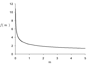
Figure 1: Universal function $f(m)$ as a function of the mass $m$ for Hamiltonian (123).

Now we calculate, still using the Lagrange mesh method, the spectrum of a system with mass $m=4$, in order to match the results of bsb08a . We think that limiting ourselves to states with $0\leq n\leq 3$ and $0\leq l\leq 3$ is enough for our purpose; the corresponding eigenenergies $\epsilon(m=4;n,l)$ are given in the first line of Table 1.

In order to calculate the effective masses $\bar{m}(4;n,l)$ as defined in (112), we need a prescription for the choice of the principal quantum number. We study here two possibilities: the HO prescription $Q(n,l)=2n+l+3/2$ and the improved value proposed in bsb08a $Q(n,l)=1.789n+l+1.375$. For both prescriptions, we calculate the effective masses (112) and insert them in the $f(m)$ function to obtain values $f(\bar{m}(4;n,l))$ which are ultimately compared to the exact results $\epsilon(4;n,l)$. The approximate values $f(\bar{m}(4;n,l))$ are reported in the second line of Table 1 for the HO prescription whereas the third line of the same Table shows the results with the improved formula. Note the the ground state is always exactly computed by definition.

Table 1: Values of $\epsilon(m=4;n,l)$ for various approximations. For each set $(n,l)$, the first line is the result obtained by numerical integration $\epsilon(4;n,l)$, the second and third lines are the results coming from duality relation $f(\bar{m}(4;n,l))$ with the HO prescription $Q(n,l)=2n+l+3/2$ and the improved prescription $Q(n,l)=1.789n+l+1.375$, respectively. Between parenthesis is also indicated the deviation (%) of the approximate result as compared to the exact ones.

$l$	$\epsilon(4;0,l)$	$\epsilon(4;1,l)$	$\epsilon(4;2,l)$	$\epsilon(4;3,l)$
0	1.473	2.575	3.478	4.275
	1.473 (0)	2.591 (0.6)	3.502 (0.7)	4.307 (0.7)
	1.473 (0)	2.567 (0.3)	3.461 (0.5)	4.251 (0.5)
1	2.117	3.077	3.911	4.665
	2.071 (2.2)	3.064 (0.4)	3.915 (0.1)	4.682 (0.3)
	2.120 (0.1)	3.083 (0.2)	3.913 (0.05)	4.662 (0.06)
2	2.676	3.546	4.327	5.046
	2.591 (3.2)	3.502 (1.2)	4.307 (0.5)	5.042 (0.08)
	2.680 (1.5)	3.559 (0.4)	4.339 (0.3)	5.055 (0.2)
3	3.182	3.989	4.728	5.416
	3.064 (3.7)	3.915 (1.8)	4.682 (1.0)	5.390 (0.5)
	3.186 (0.1)	4.005 (0.4)	4.746 (0.4)	5.434 (0.3)

From the table one sees that the duality relation (115) is very well satisfied in any case. The very simple HO prescription is less good (specially for large $l$ values) but remains acceptable with discrepancies around 1%. The improved prescription, which raises the degeneracy, is very impressive (even for large $l$ values) with an average precision of the order of 0.5%.

We checked also the validity of this duality relation for other types of potential (square root [$\sqrt{r^{2}+a}$], funnel [$-a/r+br$]) and find that the accuracy is always of the order of 1% or better. Thus, we think that the studied duality relation is well adapted for the spectrum of a two-body problem.

VI.1.3 Testing a three-body system

In this section, we test the duality relation (118) for three particles, with a mass $m$, interacting with a pure linear potential $V(r)=r$, so that the corresponding Hamiltonian in reduced variables is simply

$$H=\sum_{i=1}^{3}\frac{\bm{p}_{i}^{2}}{2m}+\sum_{i<j=1}^{3}|\bm{r}_{i}-\bm{r}_{j}|.$$ (124)

To compute the solutions of this Hamiltonian, we use a variational method relying on the expansion of trial states with a HO basis hobasis . We can write

$$|\psi\rangle=\sum_{B=0}^{B_{\textrm{max}}}\sum_{q(B)}|\phi(B,q(B))\rangle,$$ (125)

where $B=2(n_{1}+n_{2})+(l_{1}+l_{2})$ characterizes the band number of the basis state and where $q$ summarizes all the quantum numbers of the state (which can depend on $B$). This procedure is specially interesting since the eigenstates of $H$ are expanded in terms of AFM eigenstates (up to a length scale factor) silv10 ; bsb10b . In practice, a relative accuracy better than $10^{-4}$ is reached with $B_{\textrm{max}}=20$. Such results are denoted “exact” in the following. Some exact eigenvalues $\epsilon$ of (124) for $m=2$ are presented in Table 2 with the quantum numbers $\{n_{1},l_{1},n_{2},l_{2}\}$ and the $B$ value of the main component in the expansion (125).

In order to compute the effective mass (117), we need a prescription for the principal quantum number. We consider two formulas. The first one is the HO result: $Q_{\textrm{HO}}=2(n_{1}+n_{2})+(l_{1}+l_{2})+3$. The second one is given by $Q_{\textrm{WKB}}=\frac{\pi}{\sqrt{3}}(n_{1}+n_{2})+(l_{1}+l_{2})+3$. This prescription comes from the fact that the ratio between the coefficients of $n$ and $l$ for a nonrelativistic particle in a linear potential is predicted to be $\pi/\sqrt{3}$ by a WKB method brau00 and the AFM bsb08a . The set of quantum numbers used for a state is fixed by the quantum numbers of the main component in the expansion (125). It is then possible to compute the energy of an excited state from (117) and (118). The corresponding values denoted $\epsilon(Q_{\textrm{HO}})$ and $\epsilon(Q_{\textrm{WKB}})$ are presented in table 2. Note the the ground state is always exactly computed by definition.

Table 2: Some exact eigenvalues $\epsilon$ of (124) for $m=2$ with the quantum numbers $\{n_{1},l_{1},n_{2},l_{2}\}$ and the $B$ value of the main component in expansion (125). The brackets indicate that two components are equally present with $n_{1}\leftrightarrow n_{2}$ and $l_{1}\leftrightarrow l_{2}$. Energies predicted by (117) and (118) are given in columns $\epsilon(Q_{\textrm{HO}})$ and $\epsilon(Q_{\textrm{WKB}})$ following the prescription chosen for the principal quantum numbers (see text). Between parenthesis is also indicated the deviation (%) of the approximate result as compared to the exact ones.

$B$	$n_{1},l_{1},n_{2},l_{2}$	$\epsilon$	$\epsilon(Q_{\textrm{HO}})$	$\epsilon(Q_{\textrm{WKB}})$
0	0,0,0,0	4.867	4.867	4.867
1	[0,1,0,0]	5.934	5.896 (0.7)	5.896 (0.7)
2	[1,0,0,0]	6.704	6.842 (2.1)	6.671 (0.5)
	0,1,0,1	6.846	6.842 (0.1)	6.842 (0.1)
	[0,2,0,0]	6.874	6.842 (0.5)	6.842 (0.5)
3	[1,1,0,0]	7.608	7.726 (1.6)	7.566 (0.6)
	1,0,0,1	7.702	7.726 (0.3)	7.566 (1.8)
	[0,2,0,1]	7.854	7.726 (1.6)	7.726 (1.6)
4	[2,0,0,0]	8.309	8.562 (3.0)	8.256 (0.6)
	1,1,0,1	8.391	8.562 (2.0)	8.410 (0.2)
	[1,2,0,0]	8.426	8.562 (1.6)	8.410 (0.2)
	0,1,1,1	8.572	8.562 (0.1)	8.410 (1.9)
	0,2,0,2	8.707	8.562 (1.7)	8.562 (1.7)

From this table one sees that the duality relation (117)-(118) is very well satisfied in any case. The very simple $Q_{\textrm{HO}}$ prescription already gives good results, but the $Q_{\textrm{WKB}}$ prescription raises partly the degeneracy and improves appreciably the global agreement.

VI.1.4 From two- to three-body ground states

Let us consider a system of particles interacting via two-body forces and let us assume that the principal quantum number of the ground state can be written $Q_{N}=\rho(N-1)$ with $\rho$ independent of $N$. It is true for the $N$-body HO with $\rho=3/2$ (see (6)). In this case, using (120) and (121), and assuming that the AFM solution is a good approximation of the true solution, we can write

$$\epsilon^{(N)}(m;\{0,0\})\approx C_{N}\epsilon(Nm/2;0,0).$$ (126)

We have then an approximate link between the ground state of $N$ particles interacting via a two-body potential and the ground state of the corresponding two-body system. We have checked that, for $N=3$, relation (126) is satisfied with an error less that 1% for $V(x)=ax$, around 1% for $V(x)=-a/x+bx$ and around 6% for $V(x)=-a/x$ (these potentials deviate more and more from a quadratic one).

The three tests performed in sections VI.1.2, VI.1.3 and VI.1.4 prove that the most general formulation of the duality relations, as expressed by (122), is indeed satisfied with a rather good accuracy of the order of a few percent, at least for $N=2,3$.

VI.2 An ultrarelativistic system

Let us consider the following ultrarelativistic Hamiltonian

$$H=\sum_{i=1}^{N}\sqrt{\bm{p}_{i}^{2}}+a\sum_{i=1}^{N}|\bm{r}_{i}-\bm{R}|,$$ (127)

which presents some interest for hadronic physics barlnc and whose AFM eigenmasses are given by $M^{(N)}_{u}(Q)=\sqrt{4NaQ}$. In silv10 , it has been shown that the accuracy of this formula can be improved as compared to the pure HO prescription in the case $N=3$ by the determination in (7) of:

• The $\gamma$ term by using an accurate variational solution for the ground state.

• The ratio $\alpha_{i}/\beta_{i}$ by using the characteristics of a WKB solution for an ultrarelativistic particle in a linear potential brau00 .

The same method can be used in the case $N=2$. Finally, we obtain

$$M^{(2)}_{u} \approx \sqrt{8aQ^{(2)}}\quad\textrm{with}\quad Q^{(2)}=\frac{\pi}{2}n+l+\frac{4}{\pi},$$ (128)

$$M^{(3)}_{u} \approx \sqrt{\frac{32}{\pi}aQ^{(3)}}\quad\textrm{with}\quad\ Q^{(3)}=\frac{\pi}{2}(n_{1}+n_{2})+l_{1}+l_{2}+3.$$ (129)

The relative errors are below 2% for (128) and below 1% for (129) (at least for quantum numbers such that $n\leq 3$ and $l\leq 3$). So,we can consider that these formulas are very close to the exact solutions.

We can now check if relation (55) is, at least approximately, verified with $N=3$ and $p=2$ for the (nearly) exact solutions of this system. A priori, we could expect that $M^{(3)}_{u}(Q^{(3)})\approx 3/2\ M^{(2)}_{u}(2Q^{(3)}/3)$. The calculation gives

$$\frac{3}{2}M^{(2)}_{u}\left(\frac{2Q^{(3)}}{3}\right)\approx\frac{3}{2}\sqrt{8a\frac{2Q^{(3)}}{3}}=\sqrt{12aQ^{(3)}}.$$ (130)

This must be compared with (129). Since $32/\pi\approx 10.2$, the relative error is around 15%.

But, we can also hope that $M^{(2)}_{u}(Q^{(2)})\approx 2/3\ M^{(3)}_{u}(3Q^{(2)}/2)$. The calculation gives

$$\frac{2}{3}M^{(3)}_{u}\left(\frac{3Q^{(2)}}{2}\right)\approx\frac{2}{3}\sqrt{\frac{32}{\pi}a\frac{3Q^{(2)}}{2}}=\sqrt{\frac{64}{3\pi}aQ^{(2)}}.$$ (131)

This must be compared with (128). Since $64/(3\pi)\approx 6.8$, the relative error is also around 15%. In these cases, we can consider that the relevance of the duality relation is demonstrated.

VI.3 An ultrarelativistic-nonrelativistic duality

The eigensolutions of these two two-body Hamiltonians

$$H_{n} = \frac{\bm{p}^{2}}{m}+ar^{2},$$ (132)

$$H_{u} = 2\sqrt{\bm{p}^{2}}+br,$$ (133)

are given respectively by

$$E_{n}(Q_{n}) = \sqrt{\frac{4a}{m}}Q_{n},\quad\textrm{with}\quad Q_{n}=2n+l+\frac{3}{2},$$ (134)

$$M_{u}(Q_{u}) \approx \sqrt{8bQ_{u}}\quad\textrm{with}\quad Q_{u}=\frac{\pi}{2}n+l+\frac{4}{\pi}.$$ (135)

Relation (134) is exact while the relative accuracy of (135) is around 1-2%. If we impose $Q_{n}=Q_{u}=Q$, the duality relation presented in Sect. V is verified by setting $2bm=aQ$ as shown above.

Let us examine what becomes this property for the genuine solutions. If we assume that $E_{n}$ is known, we can compute the exact solutions of $H_{u}$ with $b=aQ_{n}/(2m)$. For $n\leq 3$ and $l\leq 3$, the relative error compared to (135) is below 10%. On the contrary, if we assume that $M_{u}$ is known, we can compute the exact solutions of $H_{n}$ with $a=2bm/Q_{u}$. For $n\leq 3$ and $l\leq 3$, the relative error compared to (134) can then reach 38%. Following the physical situation considered, the accuracy of this kind of duality relation can strongly vary. But, in some cases, the error could be quite small.

VII Conclusions

In this paper, we investigate the possible relationships between the energies of particular states for a given system and the energies of other states for another system. We call these relationships “duality relations”. Systems with arbitrary number of particles are considered but in a well defined framework. The basic hypotheses are the following ones:

• All the particles of the studied systems are identical.

• We do not take into account internal degrees of freedom for particles and, for convenience, we focus only on bosons in applications (the case of fermions can be dealt with as well, but it is more involved and is not studied in this work).

• We consider the kinetic energy operator either of a nonrelativistic form or of a semirelativistic form.

• We limit ourselves to one-body and two-body types of potentials.

• The potentials do not lead to coupled channel equations, so that we are faced with a Schrödinger equation for a nonrelativistic kinetic energy, and with a spinless Salpeter equation for a semirelativistic kinetic energy.

• The potentials entering the formalism do not depend on the mass $m$ nor on the number of particles $N$.

Despite the limitations, the number of systems which can be concerned by this work is quite large and may represent a lot of different physical situations.

As an intermediate tool, we introduce the auxiliary field method (AFM) to get approximate values of the eigenenergies. The important parameters are the mass $m$ and the principal quantum number $Q(\{n_{i},l_{i}\})$, function of the various radial quantum numbers $n_{i}$ and orbital quantum numbers $l_{i}$. The form of this function is not given by the theory and is left to the cleverness of the physicist. Usually, the harmonic oscillator prescription (6) is a good starting point, but a more elaborated formula, such as the one given by (7), can improve substantially the quality of the results. The AFM provides an expression $E^{(N)}(m;Q)$ of the eigenenergies (or eigenmasses for a semirelativistic kinematics) in terms of these parameters. In a series of papers bsb08a ; bsb08b ; AFMeigen ; bsb09a ; Sem09a ; bsb09c ; silv10 ; bsb10b , we proved that, the AFM approximation can be calculated analytically for many systems and leads to encouraging results.

A duality relation is, at the beginning, a link between AFM approximations $E^{(N)}(m;Q)$ and $E^{(p)}(m^{\prime};Q^{\prime})$. The case $p=2$ is particularly important because the corresponding duality relation allows to obtain the spectrum of a $N$-body system in terms of the spectrum of a 2-body system, a much more favorable situation. We obtained very general duality relations when only one-body or two-body potentials are present. More interesting conclusions can be drawn in the ultrarelativistic limit ($m=0$) or in the nonrelativistic limit. In these particular cases, we showed that the AFM results can be expressed in term of a unique universal function for a given potential and for a given kinematics. This crucial feature has a lot of important consequences for the duality relations. We proved for example that the spectrum of a nonrelativistic system governed by a two-body potential (the same property holds for a one-body potential) $V(r)$ is the same as the spectrum of an ultrarelativistic system governed by a two-body potential $W(r)=V(\alpha\sqrt{r})$ provided that the parameter $\alpha$ is chosen adequately. The nonrelativistic kinematics allows additional sympathetic features. In particular, it was shown that the spectrum of such a $N$-body system can be obtained from the ground state of the corresponding two-body system.

The duality relations presented here are exact for the AFM approximation of the eigenenergies. Assuming that this approximation leads to results close to the exact ones, the duality relations can also be applied to the exact states. This means that we have an approximate link between the exact energies of a $N$-body system $\epsilon^{(N)}(m;\{n_{i},l_{i}\})$ and the exact energies of a $p$-body system $\epsilon^{(p)}(m^{\prime};\{n^{\prime}_{i},l^{\prime}_{i}\})$. The case $p=2$ is specially interesting because nowadays we are able to get easily the spectrum of a two-body system numerically with a great accuracy.

In particular, for a nonrelativistic system, we obtained a very important conclusion. The whole spectrum of any system (arbitrary $N$ value) can be calculated, approximatively, through a universal function $f(m)$ which is nothing else than the dependence of the ground state of the two-body system (with the same potential) on the mass. This function is very easy to obtain numerically in any circumstances. The duality relation is expressed by equation (122). It is sufficient for obtaining the searched value $\epsilon^{(N)}(m;\{n_{i},l_{i}\})$ to calculate the universal function for an argument $M(m;\{n_{i},l_{i}\})$ given by (121).

The important point that we want to stress is the following one. The duality relations are exact for the AFM approximations of the eigenenergies while they are only approximately true for the exact eigenenergies (the quality probably deteriorates with increasing values of $N$). This drawback is compensated by the fact that the corresponding duality relations concern the exact eigenenergies without any reference to the AFM expressions which were only an intermediate tool. Thus, the consequences of duality relations would remain true independently of the AFM approximations. We propose to apply all the duality relations presented above for the exact eigenvalues, but only in an approximate way.

The duality relations have been tested in a number of interesting cases. In particular, using a linear potential for $N=2$ and 3, we showed that they are fulfilled with an accuracy of the order of 1-4%. For other types of potentials, for larger values of $N$ and quantum numbers $\{n_{i},l_{i}\}$, the quality is likely poorer, but we think that these duality relations are nevertheless able to give valuable informations concerning complicated systems which are not easy to be dealt with, analytically or numerically.

Appendix A Tests of duality relations for AFM energies

In order to test the duality relations presented above, we can use the semirelativistic $N$-body harmonic oscillator studied in silv10

$$H=\sum_{i=1}^{N}\sqrt{\bm{p}_{i}^{2}+m^{2}}+k\sum_{i=1}^{N}|\bm{r}_{i}-\bm{R}|^{2}+\rho\sum_{i<j=1}^{N}|\bm{r}_{i}-\bm{r}_{j}|^{2}.$$ (136)

The AFM solutions, for the general, the ultrarelativistic and the nonrelativistic cases respectively, are given by

$$M^{(N)} = \frac{2Nm}{\sqrt{3Y_{N}}}\left[\frac{1}{G_{-}(Y_{N})}+G_{-}(Y_{N})^{2}\right]\quad\textrm{with}\quad Y_{N}=\frac{4m^{2}}{3}\left(\frac{2N^{2}}{(k+\rho N)Q^{2}}\right)^{2/3},$$ (137)

$$M^{(N)}_{u} = \frac{3}{2}\left[2N(k+\rho N)Q^{2}\right]^{1/3},$$ (138)

$$E^{(N)} = \sqrt{\frac{2}{m}(k+\rho N)}Q.$$ (139)

Let us mention that the last formula is an exact solution. The function $G_{-}(Y)$ is the root of a quartic polynomial whose explicit form is given in bsb09c for instance. Using these formulas, it is easy to check the relations (23), (33), (38), (55), (62), (65), (75), (81)-(83), (87)-(90), (93)-(96).

The semirelativistic harmonic oscillator with one variable, studied in bsb09c , has the following form

$$H=\sigma\sqrt{\bm{p}^{2}+m^{2}}+ar^{2}.$$ (140)

The AFM solutions, for the general and the ultrarelativistic cases respectively, are given by

$$M^{(s)} = \frac{2\sigma m}{\sqrt{3Y_{s}}}\left[\frac{1}{G_{-}(Y_{s})}+G_{-}(Y_{s})^{2}\right]\quad\textrm{with}\quad Y_{s}=\frac{m^{2}}{3}\left(\frac{16\sigma}{aQ^{2}}\right)^{2/3},$$ (141)

$$M^{(s)}_{u} = 3\left(\sqrt{a}\frac{\sigma}{2}Q\right)^{2/3}.$$ (142)

Using these formulas, it is easy to check the supplementary relations (34)-(36), (57), (58), (63), (64).

To check the duality relations between ultrarelativistic and nonrelativistic systems with an example, we can consider the following Hamiltonian

$$H=\sum_{i=1}^{N}\sqrt{\bm{p}_{i}^{2}+m^{2}}+\textrm{sgn}(\lambda)a\sum_{i=1}^{N}|\bm{r}_{i}-\bm{R}|^{\lambda}+\textrm{sgn}(\lambda)b\sum_{i<j=1}^{N}|\bm{r}_{i}-\bm{r}_{j}|^{\lambda}.$$ (143)

Defining the quantities

$$A_{\lambda}=a|\lambda|\left(\frac{N}{Q}\right)^{\frac{2-\lambda}{2}}\quad\textrm{and}\quad B_{\lambda}=b|\lambda|N\left(\frac{N-1}{2Q}\right)^{\frac{2-\lambda}{2}},$$ (144)

the AFM solutions, for the nonrelativistic and the ultrarelativistic cases respectively, are given by silv10

$$E^{(N)} = \frac{\lambda+2}{2\lambda}Q\left[\frac{(A_{\lambda}+B_{\lambda})^{2}}{m^{\lambda}}\right]^{\frac{1}{\lambda+2}},$$ (145)

$$M^{(N)}_{u} = \frac{\lambda+1}{\lambda}\left[Q^{\lambda+2}N^{\lambda}(A_{\lambda}+B_{\lambda})^{2}\right]^{\frac{1}{2(\lambda+1)}}.$$ (146)

Using these relations with potentials $W(x)\propto x^{\lambda}$ and $U(x)\propto x^{2\lambda}$, the two theorems presented in Sect. V can be checked.

References

- (1) P. A. M. Dirac, Lectures on Quantum Mechanics (Belter Graduate School of Sciences, Yeshiva University, New York, 1966).
- (2) L. Brink, P. Di Vecchia, P. S. Howe, Nucl. Phys. B118, 76 (1977).
- (3) S. Deser, B. Zumino, Phys. Lett. B 65, 369 (1976).
- (4) A. M. Polyakov, Phys. Lett. B 103, 207 (1981).
- (5) B. Silvestre-Brac, C. Semay, F. Buisseret, J. Phys. A 41, 275301 (2008) [arXiv:0802.3601].
- (6) B. Silvestre-Brac, C. Semay, F. Buisseret, J. Phys. A 41, 425301 (2008) [arXiv:0806.2020].
- (7) C. Semay, B. Silvestre-Brac, J. Phys. A 43, 265302 (2010) [arXiv:1001.1706].
- (8) B. Silvestre-Brac, C. Semay, F. Buisseret, J. Phys. A 42, 245301 (2009) [arXiv:0811.0287].
- (9) C. Semay, F. Buisseret, B. Silvestre-Brac, Phys. Rev. D 79, 094020 (2009) [arXiv:0812.3291]; [arXiv:0901.4614].
- (10) B. Silvestre-Brac, C. Semay, F. Buisseret, Int. J. Mod. Phys. A 24, 4695 (2009) [arXiv:0903.3181].
- (11) B. Silvestre-Brac, C. Semay, F. Buisseret, F. Brau, J. Math. Phys. 51, 032104 (2010) [arXiv:0908.2829].
- (12) B. Silvestre-Brac, C. Semay, F. Buisseret, arXiv:1101.5222.
- (13) G. S. Bali, Phys. Rep. 343, 1 (2001) [hep-ph/0001312].
- (14) F. Buisseret, C. Semay, Phys. Rev. D 82, 056008 (2010) [arXiv:1006.4729].
- (15) C. Semay, D. Baye, M. Hesse, B. Silvestre-Brac, Phys. Rev. E 64, 016703 (2001).
- (16) S. Fleck, B. Silvestre-Brac, J.-M. Richard, Phys. Rev. D 38, 1519 (1988); B. Silvestre-Brac, Few-Body Syst. 20, 1 (1996).
- (17) F. Brau, Phys. Rev. D 62, 014005 (2000) [hep-ph/0412170].