Thermal Segregation Beyond Navier-Stokes

Abstract

A dilute suspension of impurities in a low density gas is described by the Boltzmann and Boltzman-Lorentz kinetic theory. Scaling forms for the species distribution functions allow an exact determination of the hydrodynamic fields, without restriction to small thermal gradients or Navier-Stokes hydrodynamics. The thermal diffusion factor characterizing sedimentation is identified in terms of collision integrals as functions of the mechanical properties of the particles and the temperature gradient. An evaluation of the collision integrals using Sonine polynomial approximations is discussed. Conditions for segregation both along and opposite the temperature gradient are found, in contrast to the Navier-Stokes description for which no segregation occurs.

I Introduction

Consider a granular mixture of two mechanically different species in a steady state with number densities $n_{0}({\bm{r})}$ and $n({\bm{r})}$, respectively. One component is dilute with respect to the other, $n_{0}({\bm{r})/}n(\mathbf{r)}<<1$, such that this component has negligible effect on the host gas. Moreover, the latter is at sufficiently low density that the granular Boltzmann kinetic theory applies for its intra-species collisions. The dilute component has negligible intra-species collisions and its collisions with the host gas are described by the granular Boltzmann-Lorentz kinetic theory RydL77 . The objective here is to provide an exact description of segregation induced by a temperature gradient in this context. The motivation is the description some years ago of an exact solution to the Boltzmann equation for a steady state with constant temperature gradient BreyFourier ; BKyR09 . That analysis is extended here to include the presence of the dilute component with a complementary description of the exact solution to the Boltzmann-Lorentz equation. Since there is no limitation on the size of the temperature gradient, the results given here extend previous results on thermal segregation obtained from the Navier-Stokes equation restricted to small gradients Garzo06 . For the dilute conditions considered here, and the absence of gravity, no segregation occurs at Navier-Stokes order in contrast to the results obtained here.

The particles of the dilute component will be referred to as the “impurities”. The hydrodynamic fields obtained for the host gas are zero flow velocity, constant temperature gradient in the $x$ direction, $dT(x)/dx=\theta$ , and a constant uniform pressure $p=n(x)T(x)$. The impurities have a temperature profile $T_{0}(x)$ proportional to the host temperature $T_{0}(x)=\gamma T(x)$, and a non-trivial density $n_{0}(x)$ expressed in terms of the host temperature field. In the dilute limit, the concentrations are $\rho_{0}(x)\simeq n_{0}(x)/n(x)$ and $\rho(x)=1-\rho_{0}(x)$. They have the relationship $d\rho_{0}/dx=-d\rho/dx$ so any spatial variation of $\rho_{0}(x)$ implies the opposite variation of $\rho(x)$ and segregation occurs. Here the segregation is induced by the temperature gradient, and it is common to introduce a thermal diffusion factor $\Lambda$ defined by

$$\Lambda\frac{d\ln T(x)}{dx}=-\frac{d\ln\rho_{0}(x)}{dx}\,.$$ (1)

This dimensionless factor depends on the properties of the two components, $\Lambda=\Lambda(\alpha,\alpha_{0},\sigma/\sigma_{0},m/m_{0},\theta^{\ast})$, where $\alpha,\alpha_{0}$ are the restitution coefficients for the host-host and impurity-host collisions, $\sigma,\sigma_{0}$ and $m,m_{0}$ are the species diameters and masses, and $\theta^{\ast}=\theta/p\sigma^{d-1}$ is the dimensionless temperature gradient, $d$ being the geometrical dimension of the system. In principle, $\Lambda$ can be positive or negative within this parameter space. The case $\Lambda=0$ implies no segregation, while $\Lambda$ positive (negative) implies the impurities increase concentration against (along) the temperature gradient. This is the thermal analogue of the Brazil nut and reverse Brazil nut effects for gravitational segregation DRyC93 ; HKyL01 ; JyY02 ; BRyM05 .

The distribution functions for the two species are of a “normal” form, meaning that their dependence on space and time occurs entirely through the hydrodynamic fields, $n(x),T(x),$ and $n_{0}(x)$ McL89 ; ByR09 . Thus, boundary conditions do not occur explicitly but only through the determination of these fields. For example, no external driving source is required in the kinetic equation for a stationary state, since this is implicit in the time independence of the fields. Instead, the stationary form of the fields is determined self-consistently from moments of the kinetic equations. This self-consistency also determines the temperature of the impurities as being proportioal to the host temperature, $T_{0}(x)=\gamma T(x)$, with $\gamma\neq 1$ in general. No reference to hydrodynamics is made, although these moment equations are equivalent to the balance equations forming the basis for a hydrodynamical description.

The steady state obtained occurs by establishing a gradient of the heat flux to compensate for local energy loss due to collisional cooling. Thus it is special to granular fluids and links the temperature gradient to the degree of inelasticity rather than to boundary conditions. This is similar to steady uniform shear flow where the steady state is possible due to a balance of viscous heating and collisional cooling, such that the velocity gradient (shear rate) is linked to the degree of inelasticity. In both cases, the control needed to assure Navier-Stokes hydrodynamics is lost. In the present case, smaller gradients entails smaller pressure at constant restitution coefficient, or smaller inelasticity at constant pressure. Such non-Newtonian steady states are a characteristic of granular flows and segregation for such states can be qualitatively different from that from Navier-Stokes hydrodynamics. This  has been illustrated recently for thermal segregation under uniform shear flow Garzo10 .

The next section defines the system and its kinetic theory description. In section III scaling forms for the distribution functions are introduced and the implications for the hydrodynamic fields are obtained. Three constants must be determined self-consistently. One of these, the temperature gradient $\theta$ has been obtained in BreyFourier ; BKyR09 . Collision integrals for the other two are obtained here. The form of the thermal diffusion factor $\Lambda$ is given in terms of these constants, and the sign of $\Lambda$ is discussed based on approximate evaluations of the collision integrals given in the Appendices.

II Kinetic theory

Consider a one component gas of $N$ smooth, inelastic hard spheres ($d=3$) or disks ($d=2$) with diameter $\sigma$ and mass $m$ at low density. Their distribution for position ${\bm{r}}$ and velocity ${\bm{v}}$ at time $t$, $f({\bm{r}},{\bm{v}},t)$, is determined from the Boltzmann equation (without external forces) GyS95

$$\left(\partial_{t}+{\bm{v}}\cdot\frac{\partial}{\partial{\bm{r}}}\right)f=J\left[{\bm{v}}|f,f\right],$$ (2)

where the collision operator $J\left[\mathbf{v}|f,f\right]$ is

$$J\left[\mathbf{v}|f,f\right]\equiv\sigma^{d-1}\int d{\bm{v}}_{1}\int d\widehat{\bm{\sigma}}\,\Theta(\widehat{{\bm{\sigma}}}\cdot{\bm{g}})(\widehat{\bm{\sigma}}\cdot{\bm{g}})\left[\alpha^{-2}f({\bm{r}},{\bm{v}}^{\prime},t)f({\bm{r}},{\bm{v}}_{1}^{\prime},t)-f({\bm{r}},{\bm{v}},t)f({\bm{r}},{\bm{v}}_{1},t)\right].$$ (3)

Here ${\bm{g}}\equiv{\bm{v}}-{\bm{v}}_{1}$ is the relative velocity of the colliding pair, $\Theta$ is the Heaviside step function, $d\widehat{\bm{\sigma}}$ is the solid angle element about the direction of the unit vector $\widehat{\bm{\sigma}}$, and $\alpha$ is the restitution coefficient characterizing the degree of inelasticity ($0<\alpha\leq 1$). The velocities ${\bm{v}}^{\prime},{\bm{v}}_{1}^{\prime}$ denote the restituting velocities for the pair ${\bm{v}},{\bm{v}}_{1}$,

$${\bm{v}}^{\prime}={\bm{v}}-\frac{1+\alpha^{-1}}{2}(\widehat{{\bm{\sigma}}}\cdot\mathbf{g})\widehat{{\bm{\sigma}}},\quad{\bm{v}}_{1}^{\prime}={\bm{v}}_{1}+\frac{1+\alpha^{-1}}{2}(\widehat{{\bm{\sigma}}}\cdot{\bm{g}})\widehat{\bm{\sigma}}.$$ (4)

Now consider $M$ additional impurity particles in this gas, all the same but mechanically different from the fluid particles. For $M\ll N$, the primary collisions for the impurity particles are with the host gas particles, and impurity-impurity collisions and effects of the impurities on the gas distribution function $f$ can be neglected. The distribution function for the impurities, $F({\bm{r}},{\bm{v}}_{0},t)$, is governed by the corresponding Boltzmann-Lorentz equation,

$$\left(\partial_{t}+{\bm{v}}_{0}\cdot\frac{\partial}{\partial{\bm{r}}}\right)F=I\left[{\bm{v}}_{0}|F,f\right],$$ (5)

where the operator $I\left[{\bm{v}}_{0}|F,f\right]$ describes changes in $F$ due to binary collisions between the impurity and gas particles,

$$I\left[{\bm{v}}_{0}|F,f\right]\equiv\overline{\sigma}^{d-1}\int d{\bm{v}}_{1}\int d\widehat{\bm{\sigma}}\,\Theta(\widehat{{\bm{\sigma}}}\cdot{\bm{g}}_{01})(\widehat{\bm{\sigma}}\cdot{\bm{g}}_{01})\left[\alpha_{0}^{-2}F({\bm{r}},{\bm{v}}_{0}^{\prime},t)f({\bm{r}},{\bm{v}}_{1}^{\prime},t)-F({\bm{r}},{\bm{v}}_{0},t)f({\bm{r}},{\bm{v}}_{1},t)\right],$$ (6)

${\bm{g}}_{01}\equiv{\bm{v}}_{0}-{\bm{v}}_{1}$. The restituting velocities ${\bm{v}}_{0}^{\prime},{\bm{v}}_{1}^{\prime}$ in this case are

$${\bm{v}}_{0}^{\prime}={\bm{v}}_{0}-\frac{m\left(1+\alpha_{0}^{-1}\right)}{m+m_{0}}(\widehat{{\bm{\sigma}}}\cdot\mathbf{g}_{01})\widehat{{\bm{\sigma}}},\quad{\bm{v}}_{1}^{\prime}={\bm{v}}_{1}+\frac{m_{0}\left(1+\alpha_{0}^{-1}\right)}{m+m_{0}}(\widehat{{\bm{\sigma}}}\cdot{\bm{g}}_{01})\widehat{\bm{\sigma}}.$$ (7)

In the above expressions, $\overline{\sigma}\equiv(\sigma+\sigma_{0})/2$, and $\sigma_{0}$, $m_{0}$, and $\alpha_{0}$ are the hard sphere diameter, mass, and restitution coefficient for the impurity particles, respectively.

The macroscopic state of this system is described by the fluid number density $n({\bm{r}},t)$, temperature $T({\bm{r}},t)$, and flow velocity ${\bm{u}}({\bm{r}},t)$, defined in terms of the distribution function by

$$\left(\begin{array}[]{c}n(\mathbf{r},t)\\ \frac{d}{2}n({\bm{r}},t)T({\bm{r}},t)\\ n({\bm{r}},t){\bm{u}}({\bm{r}},t)\end{array}\right)\equiv\int d{\bm{v}}\left(\begin{array}[]{c}1\\ \frac{1}{2}mV^{2}\\ \mathbf{v}\end{array}\right)f({\bm{r}},{\bm{v}},t),$$ (8)

with ${\bm{V}}({\bm{r}},t)\equiv{\bm{v}}-{\bm{u}}({\bm{r}},t)$. It is convenient to introduce corresponding fields for a macroscopic description of the impurity particles,

$$\left(\begin{array}[]{c}n_{0}({\bm{r}},t)\\ \frac{d}{2}n_{0}({\bm{r}},t)T_{0}({\bm{r}},t)\\ \mathbf{j}_{0}({\bm{r}},t)\end{array}\right)\equiv\int d\mathbf{v}_{0}\left(\begin{array}[]{c}1\\ \frac{1}{2}mV_{0}^{2}\\ {\bm{v}}_{0}\end{array}\right)F({\bm{r}},{\bm{v}}_{0}),$$ (9)

with ${\bm{V}}_{0}({\bm{r}},t)={\bm{v}}_{0}-\mathbf{u}_{0}({\bm{r}}_{0},t).$ Instead of an impurity velocity, the more usual number flux notation ${\bm{j}}_{0}=n_{0}{\bm{u}}_{0}$ has been used.

III Scaling solutions

In reference BreyFourier , a solution to the Boltzmann equation was described for the special case of a scaling form in terms of the hydrodynamic variables,

$$f(x,{\bm{v}})=n(x)\left[\frac{m}{2T(x)}\right]^{d/2}\phi\left({\bm{c}}\right),\quad{\bm{c}}\equiv\left[\frac{m}{2T(x)}\right]^{1/2}{\bm{v}.}$$ (10)

Such a solution, where the space and time dependence of the distribution function occurs only through the hydrodynamic fields, is called “normal”. The definitions of the fields in (8), and the choice of ${\bm{u}}=0$ give the self-consistency conditions on $\phi\left({\bm{c}},\right)$

$$\left(\begin{array}[]{c}1\\ \frac{d}{2}\\ 0\end{array}\right)=\int d\mathbf{c}\left(\begin{array}[]{c}1\\ c^{2}\\ \mathbf{c}\end{array}\right)\phi\left(\mathbf{c}\right).$$ (11)

Here, a similar scaling solution for the impurities is sought,

$$F(x,{\bm{v}}_{0})=n_{0}(x)\left[\frac{m_{0}}{2T_{0}(x)}\right]^{d/2}\Phi\left({\bm{c}}_{0}\right),\quad{\bm{c}}_{0}=\left[\frac{m_{0}}{2T_{0}(x)}\right]^{1/2}{\bm{v}}_{0}.$$ (12)

The definitions (9) then give the conditions on $\Phi$,

$$\left(\begin{array}[]{c}1\\ \frac{d}{2}+\frac{m_{0}j_{0}^{2}}{2T_{0}n_{0}^{2}}\\ \frac{1}{n_{0}}(\frac{m_{0}}{2T_{0}})^{1/2}{\bm{j}}_{0}\end{array}\right)\equiv\int d{\bm{c}}_{0}\left(\begin{array}[]{c}1\\ c_{0}^{2}\\ {\bm{c}}_{0}\end{array}\right)\Phi\left({\bm{c}}_{0}\right).$$ (13)

In order for (12) to be “normal”, it should depend only on the hydrodynamic fields for the gas and impurities, i.e., on $n_{0}(x)$, $n(x)$, and $T(x)$. Dimensional analysis then requires that $T_{0}(x)$ must be proportional to $T(x)$,

$$T_{0}(x)=\gamma T(x).$$ (14)

The constant $\gamma$ must be determined in course of solving the kinetic equation (as discussed below). Further comments on the implications of normal solutions is provided in the last section.

In terms of these scaling solutions and dimensionless velocity variables, the Boltzmann and Boltzmann-Lorentz equations become

$$c_{x}\left\{\frac{1}{n\sigma^{d-1}}\frac{d\ln n}{dx}\phi\left({\bm{c}}\right)-\frac{1}{2n\sigma^{d-1}}\frac{d\ln T}{dx}\frac{\partial}{\partial{\bm{c}}}\cdot\left[{\bm{c}}\phi\left({\bm{c}}\right)\right]\right\}=\mathcal{J}\left[{\bm{c}}|\phi,\phi\right],$$ (15)

$$c_{0x}\left\{\frac{1}{n\overline{\sigma}^{d-1}}\frac{d\ln n_{0}}{dx}\Phi\left({\bm{c}}_{0}\right)-\frac{1}{2n\overline{\sigma}^{d-1}}\frac{d\ln T}{dx}\frac{\partial}{\partial{\bm{c}}_{0}}\cdot\left[{\bm{c}}_{0}\Phi\left({\bm{c}}_{0}\right)\right]\right\}=\mathcal{I}\left[{\bm{c}}_{0}|\Phi,\phi\right],$$ (16)

with the dimensionless collision operators

$$\mathcal{J}\left[{\bm{c}}|\phi,\phi\right]\equiv\int d{\bm{c}}_{1}\int d\widehat{\bm{\sigma}}\,\Theta(\widehat{{\bm{\sigma}}}\cdot{\bm{w}})(\widehat{\bm{\sigma}}\cdot{\bm{w}})\left[\alpha^{-2}\phi\left({\bm{c}}^{\prime}\right)\phi\left({\bm{c}}_{1}^{\prime}\right)-\phi\left({\bm{c}}\right)\phi\left({\bm{c}}_{1}\right)\right],$$ (17)

$$\mathcal{I}\left[{\bm{c}}_{0}|\Phi,\phi\right]=\int d{\bm{c}}_{1}\int d\widehat{\bm{\sigma}}\,\Theta(\widehat{{\bm{\sigma}}}\cdot{\bm{w}}_{0})(\widehat{\bm{\sigma}}\cdot{\bm{w}}_{0})\times\left[\alpha_{0}^{-2}\Phi\left({\bm{c}}_{0}^{\prime}\right)\phi\left({\bm{c}}_{1}^{\prime}\right)-\Phi\left({\bm{c}}_{0}\right)\phi\left({\bm{c}}_{1}\right)\right].$$ (18)

The relative velocities ${\bm{w}}$ and ${\bm{w}}_{0}$ are now

$${\bm{w}}\equiv{\bm{c}}-{\bm{c}}_{1},\quad{\bm{w}}_{0}\equiv{\bm{c}}_{0}-\left(\frac{m_{0}}{m\gamma}\right)^{1/2}{\bm{c}}.$$ (19)

The expressions of the dimensionless restituting velocities in Eq. (18) are given in Eq. (39). Since the right sides of Eqs. (15) and (16) are independent of $x$, the left sides must be as well. This will be true if the hydrodynamic fields $n(x)$, $n_{0}(x)$, and $T(x)$ satisfy the equations

$$\frac{1}{n\sigma^{d-1}}\frac{d\ln n}{dx}=A,\quad\frac{1}{n\sigma^{d-1}}\frac{d\ln T}{dx}=B,\quad\frac{1}{n\overline{\sigma}^{d-1}}\frac{d\ln n_{0}(x)}{dx}=C,$$ (20)

where $A$, $B$, and $C$ are constants. The constants $A$ and $B$ are determined by taking moments of the Boltzmann equation (15). Namely, multiplication of the equation by $1$, $c_{x}$, and $c^{2}$, and integration over ${\bm{c}}$ yields

$$\left(A+\frac{B}{2}\right)\int d{\bm{c}}\,c_{x}\phi\left({\bm{c}}\right)=0,\quad\left(A+B\right)\int d{\bm{c}}\,c_{x}^{2}\phi\left({\bm{c}}\right)=0,$$ (21)

$$\left(A+\frac{3B}{2}\right)\int d{\bm{c}}\,c^{2}c_{x}\phi\left({\bm{c}}\right)=\int d{\bm{c}}\,c^{2}\mathcal{J}\left[{\bm{c}}|\phi,\phi\right].$$ (22)

The zeroes on the right sides of (21) result from conservation of particle number and momentum by the collision operator. The first equation of (21) is satisfied because of conditions (11) required on $\phi({\bm{c}})$, while the second equation gives $A=-B$. Finally, Eq.  (22) determines $B$,

$$B=\frac{2\int d{\bm{c}}\,c^{2}\mathcal{J}\left[{\bm{c}}|\phi,\phi\right]}{\int d{\bm{c}}\,c^{2}c_{x}\phi\left({\bm{c}}\right)}.$$ (23)

The exact hydrodynamic fields for the gas are now given exactly by ${\bm{u}}=0$ and

$$\frac{dp}{dx}=0,\quad\frac{dT}{dx}=\theta,$$ (24)

where $p=n(x)T(x)$ is the uniform pressure, and $\theta\equiv Bp\sigma^{d-1}$ is the constant temperature gradient.

A similar analysis applies for the impurity constants $C$ and $\gamma$. Taking moments of the Boltzmann-Lorentz equation (16) with respect to $1,c_{0x}\mathbf{,}$ and $c_{0}^{2}$ gives

$$\left(C+\frac{\sigma^{d-1}}{2\overline{\sigma}^{d-1}}B\right)j_{0x}=0,$$ (25)

$$C+\frac{\sigma^{d-1}}{\overline{\sigma}^{d-1}}B=\frac{\int d{\bm{c}}_{0}\,c_{0x}\mathcal{I}\left[{\bm{c}}_{0}|\Phi,\phi\right]}{\int d{\bm{c}}\,_{0}c_{0x}^{2}\Phi\left({\bm{c}}_{0}\right)}\,,$$ (26)

$$C+\frac{3\sigma^{d-1}}{2\overline{\sigma}^{d-1}}B=\frac{\int d{\bm{c}}_{0}\,c_{0}^{2}\mathcal{I}\left[{\bm{c}}_{0}|\Phi,\phi\right]}{\int d{\bm{c}}_{0}c_{0}^{2}c_{0x}\Phi({\bm{c}}_{0})}\,.$$ (27)

The right hand sides of Eqs. (26) and (27) depend on $\gamma$ explicitly through ${\bm{w}}_{0}$ (see (19)) and implicitly on both $\gamma$ and $C$ through $\Phi$. Since $B$ is known independently from Eq. (23), the two unknowns $\gamma$ and $C$ are determined by Eqs. (26) and (27). Equation (25) has two solutions, $j_{0x}=0$ and $C=-\sigma^{d-1}B/2\overline{\sigma}^{d-1}$. The latter gives an additional equation for $\gamma$ and $C$ and the problem is overdetermined. Probably, this choice is not consistent with the assumption (12). Here, it is assumed that the boundary conditions enforce the choice $j_{0x}=0$.

In summary, the description of the gas and impurities is completely specified by the kinetic equations for $\phi\left({\bm{c}}\right)$ and $\Phi\left({\bm{c}}_{0}\right)$,

$$-Bc_{x}\left\{\phi\left({\bm{c}}\right)+\frac{1}{2}\frac{\partial}{\partial{\bm{c}}}\cdot\left[{\bm{c}}\phi\left({\bm{c}}\right)\right]\right\}=\mathcal{J}\left[{\bm{c}}|\phi,\phi\right],$$ (28)

$$c_{0x}\left\{C\Phi\left({\bm{c}}_{0}\right)-\frac{\sigma^{d-1}B}{2\overline{\sigma}^{d-1}}\frac{\partial}{\partial{\bm{c}}_{0}}\cdot\left[{\bm{c}}_{0}\Phi\left({\bm{c}}_{0}\right)\right]\right\}=\mathcal{I}\left[{\bm{c}}_{0}|\Phi,\phi\right],$$ (29)

and the constants $B$, $C$, and $\gamma$ are determined self-consistently from Eqs. (23), (26), and (27). The corresponding collision integrals are further simplified in Appendix A. The hydrodynamic fields have the simple spatial forms

$$T(x)=T(0)+\theta x,\quad n(x)=\frac{p}{T(0)+\theta x}\,,$$ (30)

$$T_{0}(x)=T_{0}(0)+\gamma\theta x,\quad n_{0}(x)=n_{0}(0)\left[1+\frac{\theta x}{T(0)}\right]^{\overline{\sigma}^{d-1}C/\sigma^{d-1}B}\,.$$ (31)

IV Segregation

The segregation of impurity particles relative to the host gas is described by the inhomogeneity of the composition $\rho_{0}(x)\simeq n_{0}(x)/n(x)$, which follows from (30) and (31)

$$\rho_{0}\left(x\right)=\frac{n_{0}(0)}{n(0)}\left[1+\frac{\theta}{T(0)}x\right]^{1+\overline{\sigma}^{d-1}C/\sigma^{d-1}B}.$$ (32)

The thermal diffusion factor of (1) is therefore

$$\Lambda=-\left(1+\frac{\overline{\sigma}^{d-1}C}{\sigma^{d-1}B}\right)=-\frac{\overline{\sigma}^{d-1}}{2\sigma^{d-1}}\frac{\int d{\bm{c}}_{0}\,c_{0x}\mathcal{I}\left[{\bm{c}}_{0}|\Phi,\phi\right]}{\int d{\bm{c}}_{0}\,c_{0x}^{2}\Phi\left({\bm{c}}_{0}\right)}\frac{\int d{\bm{c}}\,c^{2}c_{x}\phi\left({\bm{c}}\right)}{\int d{\bm{c}}\,c^{2}\mathcal{J}\left[{\bm{c}}|\phi,\phi\right]}\,.$$ (33)

If the impurities are mechanically equivalent to the host particles, then $\mathcal{I}\left[{\bm{c}}_{0}|\Phi,\phi\right]=\mathcal{J}\left[{\bm{c}}|\phi,\phi\right],$ $\Phi=\phi,$ and $\Lambda=0$, since the first integral in the numerator of (33) vanishes by conservation of momentum.

The corresponding result for the thermal diffusion factor obtained from the Navier-Stokes order Chapman-Enskog solutions to the Boltzmann and Boltzmann-Lorentz equations gives $\Lambda=0$ for all values of the parameters $\alpha,\alpha_{0},\sigma/\sigma_{0},m/m_{0},\theta/p\sigma^{d-1}$. If the Navier-Stokes calculation is extended to include effects of gravity the condition becomes Garzo06

$$\left(\Lambda\frac{\partial T}{\partial x}\right)_{NS}=mg\left(\frac{T_{0}}{T}-\frac{m_{0}}{m}\right).$$ (34)

Thus thermal segregation can occur, facilitated by gravity, and depends on the sign of $\left(T_{0}/T-m_{0}/m\right)$ and the direction of $\partial T/\partial x$ relative to the gravitational force. This is in sharp contrast to the results obtained in the next section.

V Approximate determination of $T_{0}/T$ and $\Lambda$

To determine the coefficients $B,C,$ and $\gamma=T_{0}/T$, the distribution functions $\phi$ and $\Phi$ are represented as truncated Sonine polynomial expansions

$$\phi\left({\bm{c}}\right) \simeq \pi^{-d/2}e^{-c^{2}}\left[1-a_{01}\left(c^{2}-dc_{x}^{2}\right)+\left(\frac{d-1}{2}\,b_{01}+\frac{3}{2}b_{10}\right)c_{x}\right.$$ (35)

$$\left.-b_{01}c^{2}c_{x}-\left(b_{10}-b_{01}\right)c_{x}^{3}\right],$$

$$\Phi\left({\bm{c}}_{0}\right) \simeq \pi^{-d/2}e^{-c_{0}^{2}}\left[1-A_{01}\left(c_{0}^{2}-dc_{0x}^{2}\right)+\left(\frac{d-1}{d}B_{01}+\frac{3}{2}B_{10}\right)c_{0x}\right.$$ (36)

$$\left.-B_{01}c_{0}^{2}c_{0x}-\left(B_{10}-B_{01}\right)c_{0x}^{3}\right].$$

The method for determining the coefficients in these expansions is described in BreyFourier and summarized for the case here in Appendix B. The numerical solutions for the case of a two-dimensional system ($d=2$) with $m=m_{0}$ and $\sigma=\sigma_{0}=\overline{\sigma}$ are shown in Figs. 7-9 as a function of $\alpha$ for several values of $\alpha_{0}$. An important general feature is that all coefficients in (35) and (36) vanish as $\alpha\rightarrow 1$. Thus the non-uniform steady state described here exists only as a consequence of the inelasticity of the host gas. Further comment on this is given in the last section below.

In the following, attention is restricted to $\sigma=\sigma_{0}=\overline{\sigma}$ and $d=2$ for several values of $m_{0}/m$, $\alpha$, and $\alpha_{0}$. It is well-established that different species of granular mixtures have different partial temperatures, even in their homogeneous cooling state (i.e., equipartition of energy does not occur) FyM02 ; DRyC93 ; GyD99 . Figures 1 and 2 show the behavior of $T_{0}/T$ for $m_{0}/m=1$ and $2$, respectively, as a function of $\alpha$ for several values of $\alpha_{0}$. The common feature is increasing $T_{0}/T$ with decreasing $\alpha$, increasing $\alpha_{0}$, and decreasing $m_{0}/m$. Figure 3 shows a broader range of $m_{0}/m$. Even for the relatively weak dissipation values of this figure, it is clear that the largest values of $T_{0}/T$ occur for small mass ratio, maximum host dissipation, and weakest impurity dissipation.

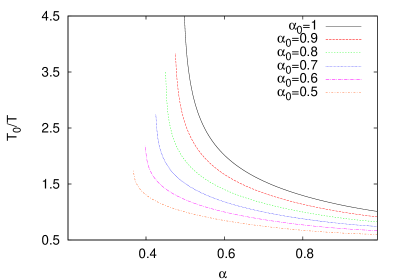
Figure 1: Temperature of the impurity $T_{0}$ divided by the temperature of the hot gas $T$ as a function of the coefficient of normal restitution of the gas particles $\alpha$, for several values of the restitution coefficient for collisions between the gas particles and the impurities, $\alpha_{0}$, as indicated in the insert. In all cases, $d=2$, $m_{0}=m$, and $\sigma=\sigma_{0}=\overline{\sigma}$.

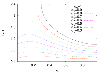
Figure 2: The same as in Fig. 1, but now $m_{0}/m=2$.

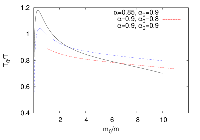
Figure 3: Temperature of the impurity $T_{0}$ divided by the temperature of the hot gas $T$ as a function of the mass ratio $m_{0}/m$ for several values of the coefficients of normal restitution $\alpha$ and $\alpha_{0}$, as indicated in the insert. In all cases, it is $d=2$ and $\sigma=\sigma_{0}.$

The existence of segregation for the same weak dissipation values of Fig. 3 is demonstrated in figure 4. The thermal diffusion factor $\Lambda$ is positive for $m_{0}/m>1$. This means that the impurity concentration is higher at the colder part of the host fluid. This is similar to the host fluid density which behaves as $n=p/T$ with constant $p$. For smaller mass ratio, segregation goes in the opposite direction with the impurity concentration highest in the hotter part of the host fluid. This effect is enhanced at stronger host fluid dissipation and weaker impurity dissipation, as illustrated in figures 5 and 6 for $m_{0}/m=1$ and $2$, respectively. It is interesting to note that for $m_{0}/m=1$ the border between the two types of segregation, $\Lambda=0$, occurs for $\alpha=\alpha_{0}$. Referring to figure 4, these values also correspond to $T_{0}/T=1$. Similarly, for $m_{0}/m=2$ comparing Figs. 2 and 6, it is seen that $\Lambda=0$ for $T_{0}/T=2$. This limited data suggest the possibility that the segregation criterion $\Lambda=0$ occurs for $m_{0}/m=T_{0}/T$. Surprisingly, this is the same as the Navier-Stokes criterion in the presence of gravity, (34). Further analysis of this potential relationship across a larger data set is required. For larger $m_{0}/m$ it is found that $T_{0}/T\leq 1$, and only the segregation for $\Lambda>0$ occurs.

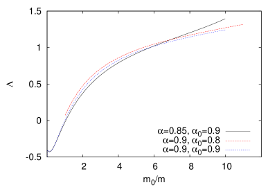
Figure 4: Dimensionless thermal diffusion factor $\Lambda$ as a function of the mass ratio $m_{0}/m$ for the same system as in Fig. 3.

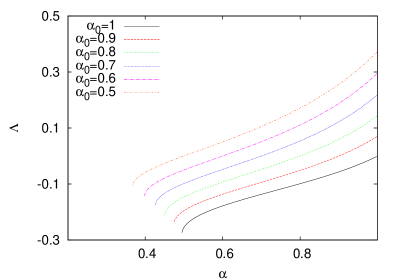
Figure 5: Dimensionless thermal diffusion factor $\Lambda$ as a function of the coefficient of normal restitution of the gas particles $\alpha$, for several values of the restitution coefficient for collisions between the gas particles and the impurities, $\alpha_{0}$, as indicated in the insert. In all cases, $d=2$, $m_{0}=m$, and $\sigma=\sigma_{0}=\overline{\sigma}$.

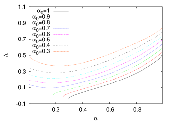
Figure 6: The same as in Fig. 5, but now $m_{0}/m=2$.

VI Discussion

The description of a low density granular gas with a dilute concentration of impurities has been given in terms of solutions to the coupled Boltzmann and Boltzmann-Lorentz kinetic equations. These are normal solutions whose space and time dependence are entirely specified in terms of the hydrodynamic fields $n,n_{0},$and $T$. The special case of a steady state in which the host gas has a constant temperature gradient and constant pressure, described earlier in refs. BreyFourier and BKyR09 , has been generalized to include a corresponding steady state of the impurities. In this way the thermal segregation factor is identified in terms of the constants of the hydrodynamic fields, without the limiting approximations of small spatial gradients. The self-consistent kinetic equations (28) and (29) determining these constants was solved using a low order Sonine polynomial approximation for the velocity dependence of the host and impurity distributions. The resulting thermal diffusion factor was found to identify conditions for both segregation along and against the temperature gradient. Such normal solutions are typically constructed by the Chapman-Enskog method whose practical application typically entails limitations to small spatial gradients, e.g. Navier-Stokes order. Application of Navier-Stokes hydrodynamics obtained in this way, and specialized to the steady state with constant temperature gradient and constant pressure, leads to the prediction of no segregation. The effects described here therefore are due to contributions from the Chapman-Enskog method beyond the small gradient approximation. In fact, there are no limitations on the temperature gradient in the present analysis.

There are two important clarifications to note. First, the validity of a normal solution both for granular and molecular gases is limited to domains away from the initial preparation time and confining boundaries. For the steady state considered here, this means that there is typically a boundary layer across which the normal solution does not apply. Additional information is then required to connect the physically specified values of the fields or their gradients at the boundary with those values associated with the normal solution. These are the familiar ”slip” boundary conditions. The existence of the normal solution described here for a system with finite confinement and associated boundary layer has been demonstrated by molecular dynamics simulation in refs.BreyFourier and BKyR09 . Typically, the size of the bulk interior relative to the boundary layer decreases as the temperature gradient is increased. Investigation of this problem for a molecular gas has demonstrated that the bulk normal solution domain still exists beyond the Navier-Stokes limit Kim89 .

A second clarification is the special nature of the steady state described here as being unique to a granular gas. The analysis of BreyFourier shows that it results from the balance of the heat flux gradient and the cooling rate due to inelastic collisions. In the absence of the latter there is no steady state solution of the type considered here. In contrast to normal fluids, the gradients of such steady states are controlled by internal processes rather than boundary sources. External control of the gradients is therefore lost. In the present case the magnitude of the dimensionless temperature gradient $\theta/p\sigma^{d-1}=B\left(\alpha\right)$ monotonically decreases to zero as $\alpha\rightarrow 1$, vanishing in the elastic limit. Consequently, for example, it is not possible for the Navier-Stokes to apply here for strong dissipation.

VII Acknowledgments

The research of JJB and NK has been partially supported by the Ministerio de Educación y Ciencia (Spain) through Grant No. FIS2008-01339 (partially financed by FEDER funds).

Appendix A Reduction of collision integrals

The Boltzmann collision integral appearing on the right side of Eq. (23) is simplified further in BreyFourier , with the result

$$B=-\frac{\left(1-\alpha^{2}\right)\pi^{(d-1)/2}}{2\Gamma\left(\frac{d+3}{2}\right)}\frac{\int d{\bm{c}}\int d{\bm{c}}_{1}\left|{\bm{c}}-{\bm{c}}_{1}\right|^{3}\phi\left({\bm{c}}\right)\phi\left({\bm{c}}_{1}\right)}{\int d{\bm{c}}\,c^{2}c_{x}\phi\left({\bm{c}}\right)}.$$ (37)

The Boltzmann-Lorentz collision integrals can be simplified in a similar way. Consider first the collision integral appearing in Eq.  (26),

$$\int d{\bm{c}}_{0}\,c_{0x}\mathcal{I}\left[{\bm{c}}_{0}|\Phi,\phi\right]=\int d{\bm{c}}_{1}\int d{\bm{c}}_{0}\,c_{0x}\int d\widehat{\bm{\sigma}}\,\Theta(\widehat{{\bm{\sigma}}}\cdot{\bm{w}}_{0})(\widehat{\bm{\sigma}}\cdot{\bm{w}}_{0})\left[\alpha_{0}^{-2}\Phi\left({\bm{c}}_{0}^{\prime}\right)\phi\left({\bm{c}}^{\prime}_{1}\right)-\Phi\left({\bm{c}}_{0}\right)\phi\left({\bm{c}}_{1}\right)\right],$$ (38)

where ${\bm{w}}_{0}$ is defined in Eq. (19) and the dimensionless restituting velocities following from Eq. (7) are

$${\bm{c}}_{0}^{\prime}={\bm{c}}_{0}-\frac{m}{m+m_{0}}\left(1+\alpha_{0}^{-1}\right)(\widehat{{\bm{\sigma}}}\cdot{\bm{w}}_{0})\widehat{{\bm{\sigma}}},\quad{\bm{c}}^{\prime}={\bm{c}}+\frac{m_{0}}{m+m_{0}}\left(1+\alpha_{0}^{-1}\right)(\frac{m\gamma}{m_{0}})^{1/2}(\widehat{{\bm{\sigma}}}\cdot{\bm{w}}_{0})\widehat{\bm{\sigma}}.$$ (39)

It is easily verified that

$$d{\bm{c}}^{\prime}_{1}{\bm{c}}_{0}^{\prime}=\alpha_{0}^{-1}d{\bm{c}}_{1}d{\bm{c}}_{0},\quad\widehat{{\bm{\sigma}}}\cdot\mathbf{g}_{0}=-\alpha_{0}\widehat{{\bm{\sigma}}}\cdot\mathbf{g}_{0}^{\prime}.$$ (40)

Also, Eqs. (39) can be inverted to get the collision rule in dimensionless units,

$${\bm{c}}_{0}^{*}={\bm{c}}_{0}-\frac{m\left(1+\alpha_{0}\right)}{m+m_{0}}(\widehat{{\bm{\sigma}}}\cdot{\bm{w}}_{0})\widehat{{\bm{\sigma}}},$$ (41)

$${\bm{c}}^{*}_{1}={\bm{c}}_{1}+\frac{m_{0}\left(1+\alpha_{0}\right)}{m+m_{0}}\left(\frac{m\gamma}{m_{0}}\right)^{1/2}(\widehat{{\bm{\sigma}}}\cdot{\bm{w}}_{0})\widehat{\bm{\sigma}}.$$ (42)

Returning to Eq. (38), change variables in the first term of the brackets on the right hand side to integrate over the restituting velocities. Using the above relations, the equation becomes

$$\int d{\bm{c}}_{0}\,c_{0x}\mathcal{I}\left[{\bm{c}}_{0}|\Phi,\phi\right] = \int d{\bm{c}}_{1}\int d{\bm{c}}_{0}\,\Phi\left({\bm{c}}_{0}\right)\phi\left({\bm{c}}_{1}\right)\int d\widehat{\bm{\sigma}}\,\Theta(\widehat{{\bm{\sigma}}}\cdot{\bm{w}}_{0})(\widehat{\bm{\sigma}}\cdot{\bm{w}}_{0})\left(c_{0x}^{*}-c_{0x}\right)$$ (43)

$$= -\frac{m\left(1+\alpha_{0}\right)}{m+m_{0}}\int d{\bm{c}}_{1}\int d{\bm{c}}_{0}\,\Phi\left({\bm{c}}_{0}\right)\phi\left({\bm{c}}_{1}\right)w_{0}w_{0x}\int d\widehat{\bm{\sigma}}\,\Theta(\widehat{{\bm{\sigma}}}\cdot{\bm{w}}_{0})(\widehat{\bm{\sigma}}\cdot\widehat{\bm{w}}_{0})^{3}$$

$$= -\frac{m\left(1+\alpha_{0}\right)}{m+m_{0}}\frac{\pi^{(d-1)/2}}{\Gamma\left(\frac{d+3}{2}\right)}\int d\mathbf{c}_{1}\int d{\bm{c}}_{0}\,\Phi\left({\bm{c}}_{0}\right)\phi\left({\bm{c}}_{1}\right)w_{0}w_{0x}.$$

Finally (26) becomes

$$C+\frac{\sigma^{d-1}}{\overline{\sigma}^{d-1}}B=-\frac{m\left(1+\alpha_{0}\right)}{m+m_{0}}\frac{\pi^{(d-1)/2}}{\Gamma\left(\frac{d+3}{2}\right)}\frac{\int d{\bm{c}}_{1}\int d{\bm{c}}_{0}\,\Phi\left({\bm{c}}_{0}\right)\phi\left({\bm{c}}_{1}\right)w_{0}w_{0x}}{\int d{\bm{c}}_{0}\,c_{0x}^{2}\Phi\left({\bm{c}}_{0}\right)}.$$ (44)

The analysis of Eq.  (27) is similar with the result

$$C+\frac{3\sigma^{d-1}}{2\overline{\sigma}^{d-1}}B=\frac{m\left(1+\alpha_{0}\right)}{m+m_{0}}\frac{\pi^{(d-1)/2}}{\Gamma\left(\frac{d+3}{2}\right)}\frac{\int d{\bm{c}}_{1}\int d{\bm{c}}_{0}\,\Phi\left({\bm{c}}_{0}\right)\phi\left({\bm{c}}_{1}\right)\left[\frac{m(1+\alpha_{0})}{m+m_{0}}\ w_{0}^{3}-2w_{0}{\bm{w}}_{0}\cdot{\bm{c}}_{0}\right]}{\int d{\bm{c}}_{0}\,c_{0}^{2}c_{0x}\Phi({\bm{c}}_{0})}\,.$$ (45)

Appendix B Solutions to kinetic equations

The solution to the kinetic equation for $\phi\left({\bm{c}}\right)$ and the self-consistent determination of $B$ is a problem that is independent of the impurities and can be carried out first. The method is described in BreyFourier . First, $B$ is given its representation as a collision integral using Eq. (23), so the kinetic equation (28) becomes

$$-2c_{x}\left\{\phi\left({\bm{c}}\right)+\frac{1}{2}\frac{\partial}{\partial{\bm{c}}}\cdot\left[{\bm{c}}\phi\left({\bm{c}}\right)\right]\right\}\frac{\int d{\bm{c}}\,c^{2}\mathcal{J}\left[{\bm{c}}|\phi,\phi\right]}{\int d{\bm{c}}\,c^{2}c_{x}\phi\left({\bm{c}}\right)}=\mathcal{J}\left[{\bm{c}}|\phi,\phi\right].$$ (46)

Next $\phi\left({\bm{c}}\right)$ is approximated by a truncated Sonine polynomial expansion

$$\phi\left({\bm{c}}\right) \simeq \pi^{-d/2}e^{-c^{2}}\left[1-a_{01}\left(c^{2}-dc_{x}^{2}\right)+\left(\frac{d-1}{2}\,b_{01}+\frac{3}{2}b_{10}\right)c_{x}\right.$$ (47)

$$\left.-b_{01}c^{2}c_{x}-\left(b_{10}-b_{01}\right)c_{x}^{3}\right].$$

This form assures the conditions given in Eq. (11). The coefficients $a_{01},b_{01}$, and $b_{10}$ are then obtained from three equations following by taking velocity moments in (46). Namely, the equation is multiplied by $c_{x}^{2},c_{x}^{3}$, and $c_{x}c^{2}$, respectively, and afterwards integrated over ${\bm{c}}$. With these coefficients determined, $B$ is calculated from Eq. (23).

To determine $\Phi\left({\bm{c}}_{0}\right)$, $C$, and $\gamma$, a similar procedure is followed. First, express $C$ as a collision integral from Eqs. (26) and (27),

$$C=2\left[\frac{3}{2}\frac{\int d{\bm{c}}_{0}\,c_{0x}\mathcal{I}\left[{\bm{c}}_{0}|\Phi,\phi\right]}{\int d{\bm{c}}_{0}\,c_{0x}^{2}\Phi\left({\bm{c}}_{0}\right)}-\frac{\int d{\bm{c}}_{0}\,c_{0}^{2}\mathcal{I}\left[{\bm{c}}_{0}|\Phi,\phi\right]}{\int d{\bm{c}}\,_{0}c_{0}^{2}c_{0x}\Phi({\bm{c}}_{0})}\right],$$ (48)

and use this in the kinetic equation (29). Next, express $\Phi\left({\bm{c}}_{0}\right)$ as a truncated Sonine polynomial expansion

$$\Phi\left({\bm{c}}_{0}\right) \simeq \pi^{-d/2}e^{-c_{0}^{2}}\left[1-A_{01}\left(c_{0}^{2}-dc_{0x}^{2}\right)+\left(\frac{d-1}{d}B_{01}+\frac{3}{2}B_{10}\right)c_{0x}\right.$$ (49)

$$\left.-B_{01}c_{0}^{2}c_{0x}-\left(B_{10}-B_{01}\right)c_{0x}^{3}\right],$$

which satisfies the conditions (13) with $\mathbf{j}_{0}=0$. The coefficients, $A_{01},B_{01}$, and $B_{10}$ are determined from three equations obtained by taking moments of (29) with respect to $c_{0x}^{2},c_{0x}^{3},$ and $c_{0x}c_{0}^{2}$. However, these equations also depend on $\gamma$, so they are supplemented by an additional equation relating the above coefficients to $\gamma$. It is obtained from a new combination of Eqs. (26) and (27)

$$B=\frac{2\overline{\sigma}^{d-1}}{\sigma^{d-1}}\left[\frac{\int d{\bm{c}}\,_{0}c_{0}^{2}\mathcal{I}\left[{\bm{c}}_{0}|\Phi,\phi\right]}{\int d{\bm{c}}_{0}\,c_{0}^{2}c_{0x}\Phi({\bm{c}}_{0})}-\frac{\int d{\bm{c}}\,_{0}c_{0x}\mathcal{I}\left[{\bm{c}}_{0}|\Phi,\phi\right]}{\int d{\bm{c}}_{0}\,c_{0x}^{2}\Phi\left({\bm{c}}_{0}\right)}\right].$$ (50)

Since $\phi$ and $B$ are known at this point, this gives four independent equations for the coefficients $A_{01},B_{01},B_{10}$, and $\gamma$. With these determined, $C$ is calculated from Eq. (48).

In practice, the above procedure leads to highly nonlinear equations for the coefficients. In the numerical results to be presented in the following, only terms up to second degree in the coefficients have been kept BKyR09 . As an example, in Figs.  7-9, the parameters obtained for a two-dimensional system ($d=2$) with $m=m_{0}$ and $\sigma=\sigma_{0}=\overline{\sigma}$ are plotted as a function of $\alpha$ for several values of $\alpha_{0}$. For small values of $\alpha$, the numerical solutions for the $B$ parameters constructed as described above seem to disappear.

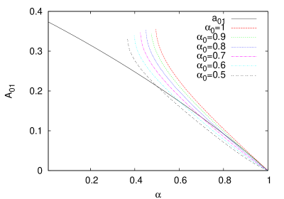
Figure 7: The dimensionless parameters $a_{01}$ and $A_{01}$ as a function of the coefficient of normal restitution of the host gas particles $\alpha$, for several values of the coefficient of restitution for the collisions between the gas particles and the impurities, $\alpha_{0}$. The coefficient $a_{01}$ does not depend on the latter. The other (fixed) parameters are $d=2$, $m_{0}=m$, and $\sigma_{0}=\sigma$.

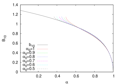
Figure 8: The same as in Fig. 1 but for the coefficients $b_{10}$ and $B_{10}$.

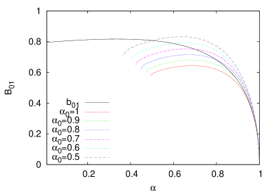
Figure 9: The same as in Fig. 1, but for $b_{01}$ and $B_{01}$.

References

(1) P. Résibois and M. de Leener, Classical Kinetic
theory of Fluids (Wiley-Interscience, New York, 1977).
(2) J. J. Brey, D. Cubero, F. Moreno, and M. J.
Ruiz-Montero, Europhys. Lett. 53 432 (2001).
(3) J. J. Brey, N. Khalil, and M. J. Ruiz-Montero, J. Stat.
Mech. P08019 (2009).
(4) V. Garzó, Europhys. Lett. 75, 521 (2006); Phys.
Rev. E78 020301(R) (2008); Eur. Phys. J. E29, 261 (2009).
(5) J. Duran, J. Rajchenbach, and E. Clément, Phys. Rev. Lett.
70, 2431 (1993).
(6) D.C. Hong, P.V. Quinn, and S. Luding, Phys. Rev. Lett.
86, 3423 (2001).
(7) J.T. Jenkins and D.K. Yoon, Phys. Rev. Lett. 88
194301 (2002).
(8) J.J. Brey, M.J. Ruiz-Montero, and F. Moreno, Phys. Rev.
Lett. 95, 098001 (2005).
(9) J.A. McLennan, Introduction to Non-equilibrium
Statistical Mechanics (Prentice Hall, New Jersey, 1989).
(10) J.J. Brey and M.J. Ruiz-Montero, Phys. Rev. E 80, 041306 (2009).
(11) V. Garzó and F. Vega Reyes, J. Stat. Mech. P07024 (2010).
(12) A. Goldshtein and M. Shapiro, J. Fluid Mech. 282,
75 (1995).
(13) K. Feitosa and N. Menon, Phys. Rev. Lett. 88, 198301 (2002).
(14) V. Garzó and J.W. Dufty, Phys. Rev. E 60, 5706 (1999).
(15) C. S. Kim and J. Dufty, Phys. Rev. A 40, 6723
(1989); C. S. Kim, J. Dufty, A. Santos, and J. J. Brey, Phys. Rev. A 40, 7165 (1989).