Luminous satellites of early-type galaxies I: Spatial distribution

Abstract

We study the spatial distribution of faint satellites of intermediate redshift ($0.1<z<0.8$), early-type galaxies, selected from the GOODS fields. We combine high resolution HST images and state-of-the-art host subtraction techniques to detect satellites of unprecedented faintness and proximity to intermediate redshift host galaxies (up to 5.5 magnitudes fainter and as close as 0$\farcs$5/2.5 kpc to the host centers). We model the spatial distribution of objects near the hosts as a combination of an isotropic, homogeneous background/foreground population and a satellite population with a power law radial profile and an elliptical angular distribution. We detect a significant population of satellites ($N_{\rm{s}}=1.7^{+0.9}_{-0.8}$) that is comparable to the number of Milky Way satellites with similar host-satellite contrast. The average projected radial profile of the satellite distribution is isothermal ($\gamma_{\rm p}=-1.0^{+0.3}_{-0.4}$), which is consistent with the observed central mass density profile of massive early-type galaxies. Furthermore, the satellite distribution is highly anisotropic (isotropy is ruled out at a $>$99.99% confidence level). Defining $\phi$ to be the offset between the major axis of the satellite spatial distribution and the major axis of the host light profile, we find a maximum posterior probability of $\phi=0$ and $|\phi|$ less than $42^{o}$ at the 68% confidence level. The alignment of the satellite distribution with the light of the host is consistent with simulations, assuming that light traces mass for the host galaxy as observed for lens galaxies. The anisotropy of the satellite population enhances its ability to produce the flux ratio anomalies observed in gravitationally lensed quasars.

—————————————————————————

1. Introduction

Cold Dark Matter (CDM) simulations have been successful at predicting the distribution of matter on super-galaxy scales (greater than a few Mpc), but less successful on smaller scales, predicting orders of magnitude more satellite galaxies than are observed in the local group (Strigari et al., 2007). The solution to the so-called missing satellite problem will have important implications for dark matter cosmology and star formation in low mass halos (Klypin et al., 1999; Moore et al., 1999). The discrepancy between observed and predicted satellite numbers could be due to incorrect assumptions about the nature of dark matter in the cosmological simulations. For instance, it has been proposed that small scale structure does not form because dark matter is not actually “cold” but instead has appreciable velocity (e.g. Colín et al., 2000), or that the power spectrum of density fluctuations used in simulations is incorrect (e.g. Kamionkowski & Liddle, 2000; Zentner & Bullock, 2003). Alternatively, it is possible that the simulations are correct but that very low mass satellites are too faint to be detected. The luminosity of satellites is difficult to predict theoretically as high resolution CDM simulations do not include baryonic interactions and therefore neglect how processes such as UV reionization, baryonic cooling, supernovae, and gas accretion affect star formation in dark matter halos (Thoul & Weinberg, 1996; Gnedin, 2000; Kaufmann et al., 2008). Hydrodynamical simulations which include gas and radiative transfer have been able to reproduce some aspects of the observed luminosity and metallicity properties of galaxies (see Springel, 2010, and references therein). However, these simulations must be improved in order to attain the complete and self-consistent understanding of star formation which is needed to predict the luminosity function of satellite galaxies.

While the luminosity and mass functions of satellites can be used to constrain cosmology and star formation, their spatial distribution can be used as a tracer of the total mass distribution of galaxy halos. Numerical simulations (Kravtsov, 2010) predict that satellites should be distributed as the mass profile of the host galaxy which, neglecting baryons, is expected to be approximately a Navarro et al. (1996, hereafter NFW) profile. However, the inner region of the host halo profile is likely to be steeper in the presence of baryons (e.g., Blumenthal et al., 1986; Gnedin et al., 2004). From gravitational lensing techniques, the total central mass density distributions of massive early-type galaxies have been shown to follow approximately isothermal profiles (i.e., $\rho(r)\propto r^{-2}$; Cohn et al., 2001; Treu & Koopmans, 2004; Koopmans et al., 2006, 2009; Auger et al., 2010). The two point correlation function of luminous red galaxies (limiting magnitude $\sim L^{*}$) in the Sloan Digital Sky Survey (SDSS) has been shown to be consistent with an isothermal satellite distribution (Watson et al., 2010, hereafter W10), although Chen (2008) (hereafter C08) studied fainter satellites with a limiting magnitude of about 0.1$L^{*}$ and found that these satellites followed a distribution closer to NFW. This apparent discrepancy in the form of the radial profile of satellites is likely due to the differences in how line-of-sight interlopers are treated in the two studies and the different radial ranges that were probed. The angular profile of satellites is also expected to follow the host mass distribution, and simulations predict that satellites will have an anisotropic spatial distribution, appearing preferentially along the major axis of the host mass profile (e.g. Zentner et al., 2005; Zentner, 2006; Knebe et al., 2004; Aubert et al., 2004; Faltenbacher et al., 2007, 2008). This anisotropy has been observed in the local group  (e.g. Metz et al., 2009) and in SDSS galaxy distributions (Brainerd, 2005; Yang et al., 2006; Wang et al., 2008; Agustsson & Brainerd, 2010).

Furthermore, the abundance of bright satellites (typically brighter than about 0.1 $L^{*}$) near hosts, also known as close pairs, has been used to constrain the rate of major mergers given assumptions about merger timescales and stellar mass to virial mass ratios (e.g. Bell et al., 2006; Patton & Atfield, 2008; Bundy et al., 2009; Robaina et al., 2010; Le Fèvre et al., 2000). Mergers are believed to play a key role in galaxy growth. For instance, simulations by Hopkins et al. (2010) indicate that about 30 percent of the mass in galaxy bulges comes from minor mergers (mergers where the mass ratio between merging objects is less than 1/3). Furthermore, observations and simulations have shown that minor mergers may play a dominant role in determining the recent (z$<1$) star formation activity in early-type galaxies (Kaviraj et al., 2009, 2011). One would therefore like to study the merger rates at lower virial and stellar mass scales (see also Bundy et al., 2007; Naab et al., 2009; Fakhouri et al., 2010), although this requires finding and studying faint satellites at cosmological distances.

Jackson et al. (2010, hereafter J10) have used high resolution Hubble Space Telescope (HST) imaging from the COSMOS survey (Scoville et al., 2007) in order to search for satellites around approximately 11,000 massive galaxies. They searched for companion objects within 2″  from their hosts, although the closest objects remained undetected as can be seen, for example, in the third panel of Figure 3 of their paper. They compared their findings to the number of satellites that have been found around 22 CLASS lens systems and found that the lens systems were more likely to have a companion object than a typical COSMOS elliptical galaxy.

The efforts of Jackson et al. (2010) highlight the difficulties of studying satellites at higher redshifts, where decreasing physical resolution reduces the number of faint companions that can be observed near bright hosts. However, one successful method of studying the mass and positional properties of high redshift satellites has been observations and simulations of gravitationally lensed active galactic nuclei (AGN) (e.g. Dalal & Kochanek, 2002; McKean et al., 2005; Vegetti et al., 2009; Xu et al., 2009). This method shows great promise with regards to the missing satellite problem because the brightness of the lensed images is very sensitive to local perturbations of the deflector potential, such as those expected from substructure. Thus, mass models which reproduce lensed image magnitudes can be used to infer the presence of satellites regardless of whether or not the satellites are luminous. However, there are two main difficulties with using lensed quasars to study satellites. The first is the small number of suitable strong lens systems currently known and the complexity of their selection function (e.g., Treu, 2010, and references therein). This limitation will become less important with new surveys such as the Large Synoptic Survey Telescope (LSST) which will vastly increase the number of detected quasar lenses (Oguri & Marshall, 2010). A second and more significant difficulty with using lensing to study satellite properties is that bright lensed images make it difficult or impossible to measure the luminosity of perturbing satellites (e.g. McKean et al., 2005), although this will be mitigated by future telescopes with higher resolution than what is currently available. In addition to AGN, recent work has shown that dark satellites can be detected by reconstructing the lensing potential using extended background sources (e.g., Koopmans, 2005; Vegetti et al., 2009, 2010), further enlarging the sample of gravitational lenses that can be used to detect substructure. Furthermore, substructure might be detectable using detailed positional and time-delay measurements of lensed images rather than just magnification (MacLeod et al., 2009) thus further addressing the first limitation.

A powerful approach to understanding star formation efficiency in low mass satellite galaxies is the combination of lensing studies to constrain the mass function of satellites, and imaging studies to constrain the luminosity function (Treu, 2010; Kravtsov, 2010, and references therein). With this goal in mind, we have started a new program to characterize the visible properties of faint satellites of massive galaxies. In this first paper, we focus on the spatial distribution of faint satellites of early-type galaxies at intermediate redshifts, $0.1<z<0.8$, selected from the GOODS fields (Giavalisco et al., 2004). We concentrate on this population of hosts because early-type galaxies dominate the sample of strong lensing galaxies (Auger et al., 2009) and are therefore the proper host sample for comparison to the satellite mass function results from lensing studies. An additional benefit to studying early-type galaxies is that they have relatively smooth surface brightness profiles which are ideal when searching for nearby compact and faint companions.

For this initial analysis we only require one photometric band. We use $z_{850}$ because it is the reddest of the GOODS bands and therefore it is the most faithful tracer of stellar mass. In forthcoming papers of this series we will use multiple band photometry to improve line-of-sight interloper removal and constrain the luminosity and stellar mass functions of the satellites (Nierenberg et al. 2011a, in preparation; hereafter paper II), and we will combine our results with the total mass function obtained from strong lensing studies to constrain the total-to-stellar mass ratio of the satellites (Nierenberg et al. 2011b, in preparation; hereafter paper III).

This paper is organized as follows: In §2 we discuss the properties of our host galaxy sample. In §3 we summarize our image analysis, including our elliptical B-spline host galaxy subtraction and faint object detection and photometry methodologies. In §4 we take a first look at the satellite distribution by means of a binned analysis, which is useful for visualizing the main trends and identifying the strength of the signal. In §5 we describe our model for the combined satellite plus background object spatial distribution and the parameters that we aim to constrain (average number of satellites, power law slope, etc.) along with a number of nuisance parameters (density of the background population, slope of the background number counts, etc.). In § 6 we present the results obtained by comparing our model to the data. In § 7 we discuss our results and compare them to previous satellite studies. In § 8 we provide a concise summary. The appendix contains more detailed explanations of many of the methods we used in this paper.

Throughout this paper, we assume a flat $\Lambda$CDM cosmology with $h=0.7$ and $\Omega_{\rm m}=0.3$. All magnitudes are given in the AB system (Oke, 1974) unless otherwise stated.

2. Host Galaxy Sample

We select a population of early-type (E and S0) host galaxies from the catalog of Bundy et al. (2005), which contains spectroscopic redshifts,stellar mass estimates, and morphological classifications for 47% of its objects (see Treu et al., 2005). The objects in this catalog were originally selected from Hubble Space Telescope photometric catalogs made by the GOODS team using the SExtractor software (Bertin & Arnouts, 1996). In the GOODS-South field, we use COMBO-17 photometric redshifts (Wolf et al., 2004) for our hosts where spectroscopic redshifts are not available. In the GOODS-North field only a handful of objects have morphological classifications and stellar mass estimates but no spectroscopic redshifts. We excluded these from our analysis.

We limit the host redshifts to $z<0.8$ to guarantee that we can detect satellites with host-satellite luminosity contrasts fainter than the equivalent contrast between the Small Magellanic Cloud and the Milky Way at all redshifts, thus increasing the likelihood that we observe approximately one satellite per host. We also exclude $z<0.1$ galaxies, which are few (owing to the small volume) and too extended in angular size to analyze in the same way as the more distant sample. Finally we exclude two hosts which appear to be undergoing major mergers as these have physical environments which are significantly distinct from the majority of our sample. To ensure that we study the same population of satellites for all hosts, despite their broad distribution in redshift, we only consider satellites brighter than a fixed fraction ($\Delta m$) of the host galaxy luminosity (i.e. a fixed difference in magnitude). We also require that all objects be brighter than the detection threshold (z₈₅₀$=m_{\rm max}=26.5$, as described in Section 3.2), and therefore we cut the parent sample to a maximum value of z₈₅₀, depending on the choice of $\Delta m$, such that $m_{\rm host}+\Delta m<m_{\rm max}$.

As we increase the size of the magnitude range we study, the number of hosts that are complete within that magnitude range drops; there are 202, 127 and 71 hosts complete to $\Delta m=$ 6.0, 5.5, and 5.0 respectively in the final host sample. At the same time, the number of satellites per host is expected to increase with $\Delta m$. The optimal choice of $\Delta m$ needs to strike a balance between the two effects. As we will show, for the present GOODS dataset we find that $\Delta m$=5.5 maximizes the signal to noise ratio of the detection and therefore we will adopt this choice as our default. To illustrate the robustness of our results to small changes in $\Delta m$, we will also describe our findings for $\Delta m$ = 5 and 6. The distributions of host redshifts, absolute magnitudes, and stellar masses for the three choices of $\Delta m$ are shown in Figure 1. As $\Delta m$ becomes larger, the hosts that satisfy the completeness requirements tend to become brighter and shift to lower redshift. As with any flux limited sample, the lower redshift objects of the sample will be dominated by the more abundant, intrinsically fainter galaxies, while the higher redshift objects will be dominated by intrinsically brighter objects. We defer an analysis of evolutionary trends to papers II and III where we will also study the luminosity and stellar mass properties of the satellites. Results in this paper are an average of the properties of the satellite population in the $0.1<z<0.8$ redshift range.

We use the second order moment of the host intensity distribution, measured along the major axis by SExtractor as a scale factor which we represent by $R_{\rm h}$. $R_{\rm h}$ compensates not only for varying angular size with redshift, but is also intrinsically related to host masses via the size-mass relation (e.g. Trujillo et al., 2006; Williams et al., 2010) and thus adjusts for variations in host masses at a given redshift. $R_{\rm h}$ varies across the host sample in physical size (0.8-5.5 kpc) with host mass variations and in angular size (between 0$\farcs$2-1$\farcs$1). The median (and modal) values of $R_{\rm h}$ are 0$\farcs$5 and 3 kpc. We use these as fiducial values when converting our results to angular and physical scales.

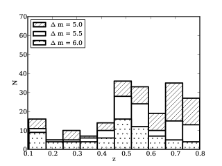
Figure 1.— From top to bottom: The distribution of host redshifts, absolute V band magnitudes, and stellar masses in three host completeness ranges ($\Delta m<m_{\rm max}-m_{\rm host}$) taken from Bundy et al. (2005).

3. Detection and photometry of close neighbors

Companions of high redshift galaxies are difficult to study because they are intrinsically faint and often obscured by the host galaxy light. In this section we describe our method of modeling and subtracting the host galaxy light profile to allow us to identify and perform accurate photometry on nearby objects. Note that while we model host light in small regions around each host, we do not limit our analysis to objects within this modeled region. We use the GOODS catalogs for photometry and astrometry for all objects outside of the modeled cutout region.

3.1. Host Galaxy B-Spline Models

Producing a good model for the light profile of the host galaxies is critical for studying the population of faint objects near the host. We use a multi-step process to create an accurate model of the host light profile which does not include the light from nearby objects.

We model the host light profile in a small cutout centered on the host galaxy. We choose this cutout to be 20 $\times$ 20 $R_{\rm h}$ in order to ensure that all significant levels of host light are removed. In the first step of the modeling process, we use SExtractor to identify all objects in the cutout region. The SExtractor parameters at this stage are chosen to err on the side of identifying noise peaks as objects in order to ensure that all real objects being obscured by the host light are recognized; see Appendix A for a detailed description of the SExtractor parameters and how they were chosen. SExtractor outputs a segmentation map which we use to mask out all identified objects other than the host galaxy. SExtractor also returns measurements of the axis ratio and position angle of the host galaxy which we use in addition to $R_{\rm h}$ to define an elliptical coordinate system for the cutout.

We then model the host light in the masked image using empirical polar B-spline models. We choose B-spline models because they quickly fit the observed light distribution with a smooth model that is independent of PSF effects and is more flexible than Sersic models, for example. Our method is similar to that described by Bolton et al. (2005, 2006). Each iteration of the B-spline code fits a model to the masked data, subtracts the model, and then identifies and masks new residual structures. This process is repeated three times. The final B-spline model is then subtracted from the data to produce a residual image, which is used to perform object detection and photometry for field galaxies near the host. Further details of the modeling and masking procedure are provided in Appendix A. Examples of our host subtraction procedure are shown in Figure 2.

3.2. Object Detection and Photometry

We use SExtractor to detect and measure the properties of objects within the host-subtracted cutouts. To ensure completeness, we limit the sample to objects with MAG_AUTO z₈₅₀$<26.5$ magnitudes, where the GOODS images are virtually 100% complete, even close to the host galaxy as we will show below. Furthermore, we only study objects fainter than z₈₅₀$>21.0$ magnitudes. This is because our analysis relies on an accurate characterization of the background (see Section 5.2) and very bright objects appear in low numbers with large fluctuations which can bias the number counts slope near a particular host.

Because we use the GOODS catalog data outside of our cutouts, it is imperative that our detections and photometry after host light subtraction are as close as possible to GOODS detections and photometry. We confirmed this by running SExtractor with our parameters on a large un-modeled section of the GOODS field. We recovered virtually the same number of objects and our photometry was consistent with GOODS photometry. This comparison is described in further detail in Appendix  B.

Due to the relative brightness of hosts compared to satellites, there is a minimum radius at which we will be able to accurately identify faint objects, regardless of how careful we are during the host modeling process.

By simulating point sources at and fainter than our chosen limiting magnitude (26.5) at varying distances from a representative subset of hosts, we find the minimum radius for completeness to be 1.5 $R_{\rm h}$ ($\sim$ 0$\farcs$9) for the vast majority of cases. The few cases for which highly flattened hosts have significant residuals extending to a larger distance are identified manually; for those systems, appropriately larger inner regions are excluded from our analysis (see Appendix A).

Note that in the redshift range we study, even the most intrinsically faint sources will have effective radii typically less than 0$\farcs$1 (see, e.g., de Rijcke et al., 2009) which is smaller than the FWHM of the GOODS PSF. Thus these sources are effectively point sources. We test our sensitivity to intrinsically faint sources by simulating faint exponential disks near our hosts at varying redshifts, with effective radii estimated from the relations given by de Rijcke et al. (2009). In the innermost region, between 1.5 and 3.5 $R_{\rm h}$, we failed to detect approximately 20% of 26.5 magnitude objects. Outside of this region we recovered approximately 100% of the simulated objects. For brighter objects with apparent magnitudes of 24.5 our recovery was approximately 100% complete even in this inner region. In our final analysis we study the satellite population between $1.5$ and 45 $R_{\rm h}$. Taking this into account, we can examine the worst case scenario in which all satellites are exponential disks with apparent magnitudes of 26.5. Assuming that satellites are distributed radially in projection as $P_{sat}(r)\propto r^{-1}$, we would only underestimate the final satellite number by 1-2 % because even in this extreme case, the incompleteness is confined to a small region. Thus we expect that the loss of completeness in the innermost region for the faintest sources will have a negligible effect on the analysis of the total sample.

To compile a single catalog and avoid duplications, we compare the position of each object identified in the residual images to objects already in the GOODS catalogs. If the object is already in the catalogs (position within 0$\farcs$3), we replace the GOODS photometry and astrometry with our own measurements, which do not suffer from being contaminated by host-galaxy light (see Figure 3). The mean distance between ‘matched’ objects was $4\pm 3$ pixels, this corresponds to 0$\farcs$12 which is the FWHM of the GOODS PSF. For objects that are not matched to objects already in the GOODS catalog, we add a new entry. Finally, for all objects outside of the host-subtracted cutouts, we use the measurements from the GOODS catalog and we do not attempt to detect new objects. In Figure 2 we show examples of the modeling process for a variety of host ellipticities and physical sizes, along with newly detected objects in the host-subtracted images.

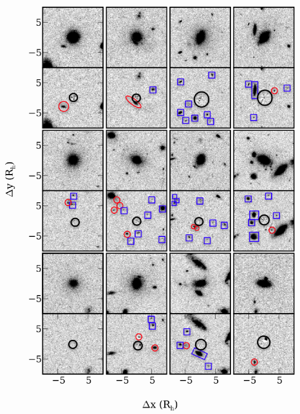
Figure 2.— Demonstration of galaxy modeling for a range of host ellipticities and sizes. Original images are shown with residuals after host model subtraction immediately below. Host galaxy physical size and ellipticity decrease downwards and to the left. All images are 20 $R_{\rm h}$ on a side. New object detections, made possible by the host light subtraction, are circled in red. Objects that were detected in the GOODS catalogs and that have complete photometry within the cutout (i.e. did not raise a SExtractor flag greater than 2) are identified by blue squares. Some objects visible to the eye were omitted from our final catalog because they were fainter than our detection limit (for instance, the object just outside of the excluded region in the top right galaxy). The central region of the host, excluded in our analysis, is identified by a black circle.

3.3. Objects Detected in Cutout Regions

The host light subtraction has two important effects on our measurement of objects near the host galaxy. The first is that it removes host light contamination and allows for accurate photometry of nearby objects, as shown in Figure 3. This figure compares GOODS photometry to host-subtracted photometry for objects that had already been identified in the GOODS catalogs. As expected, we measure object magnitudes to be slightly fainter than the GOODS photometry after host subtraction, with a mean difference of 0.12 $\pm$ 0.02 magnitudes for objects within 8 $R_{\rm h}$ ($\sim$ 4″) of the host galaxy. Our photometry is identical to GOODS photometry without host subtraction (see Appendix B), and we confirmed that the host light removal was accurate by simulating faint point sources near the hosts and ensuring that they were recovered with accurate photometry. Thus the difference in magnitude after host subtraction shown in Figure 3 is entirely due to the removal of the host light contamination which has a significant impact on photometry performed near bright objects.

Figure 3.— Comparison of photometry before (z_850,G) and after ($z_{850}$) host subtraction for objects in cutout regions which had already been identified in the GOODS catalogs prior to host subtraction.

The second important effect of host light subtraction is that it allows us to detect new objects. If the newly detected objects are real rather than artifacts of the host light subtraction, then we expect that object properties such as brightness and elongation will be similar to the properties of objects that had already been detected in the GOODS fields. The effect of weak lensing on magnification and shear is negligible for the small number of background sources close to the host Einstein radii in projection (the affected region is typically an annulus of $\sim$ 1$\farcs$0 $\pm$ 0$\farcs$2 for massive ellipticals). One way to see this is using the fact that the effect of weak lensing on the background number counts goes as $N_{\rm obs}/N_{\rm true}=1/\mu^{(\beta-1)}$ where $\mu$ is the magnification due to the host galaxy and $\beta$ is the power-law slope of the faint end of the background galaxy flux distribution (see Equation 111 of Part 1 of Schneider, Kochanek and Wambsganss 2006). In the case of $z_{850}$, $\beta$ is fairly close to one (about 0.7) and thus we do not expect weak lensing to have a significant impact on our object detection.

In the top panel of Figure 4, we compare the distributions of the axis ratios of the GOODS catalog sources and the newly detected objects near the host galaxies. The two distributions are indistinguishable, with a Komogorov-Smirnoff (KS) probability of being drawn from the same distribution of 0.96. The second panel of Figure 4 shows the distribution of contrast in MAG_AUTO ($\delta$m$=m-m_{\rm h}$) between host and detected objects. Note the use of lower-case $\delta$, which denotes a specific contrast from the host and is different from $\Delta m$ which describes the allowed maximum contrast between host and neighboring objects for a particular data set. The KS value for the two distributions being the same is $0.14$. This value is low, but not low enough to rule out the possibility that the distributions are the same. Note that our improved host galaxy light subtraction procedure is important for detecting companion objects fainter than about $\delta$m$=2.5$ magnitudes (which is about 0.5 magnitudes fainter than the magnitude contrast between the Milky Way and the Large Magellanic Cloud).

As expected, the number density radial profiles are very different for newly detected objects and objects that had already been detected in GOODS (bottom panel of Figure 4), with a KS probability of $6.0\cdot 10^{-25}$ for new and GOODS objects being drawn from the same spatial distribution. The number density of new detections increases steadily towards the center of the host, while the number density of objects already in the GOODS catalogs decreases. Host light subtraction triples the number density of detected objects in the inner 3″.

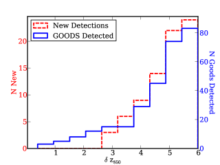
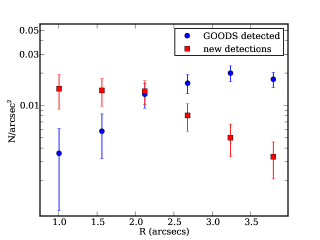
Figure 4.— Comparison of the properties of objects detected in the GOODS catalogs to those of newly detected objects. Top: The distribution of object ellipticities ($1-q=1-b/a$). Middle: The distribution of magnitude differences from hosts ($\delta$m$=m-m_{h}$). Bottom: Number density of objects as a function of distance from the host. Newly detected objects are closer to the host than those in the GOODS catalogs.

4. First Look

The host light subtraction discussed in Section 3 allows us to create an enhanced catalog of objects near the host galaxies. In this section, we show the radial and angular profiles of objects in spatial bins in order to provide a qualitative sense of the properties of objects near the hosts. Binning is useful because it provides a visual representation of data. However, it is inherently limited because it requires data points to be averaged, thereby losing valuable information. Thus we do not perform our analysis on the binned data but instead use this section to justify our model choices in Section 5.

4.1. Radial Distribution

Figure 5.— Average number density of objects as a function of distance from the host in units of the second order moment of the host intensity profile along the major axis ($R_{\rm h}$).

In Figure 5 we show the average number density of objects as a function of distance from the hosts. The number density of sources increases dramatically near the hosts. At large radii the number density becomes dominated by the isotropic and homogeneous distribution of objects not associated with the hosts. In Section 5 we will describe how we analyze the number density signal by inferring the combined properties of the satellite and background/foreground populations.

4.2. Angular Distribution

In Figure 6 we plot the angular distribution of objects within 20 $R_{\rm h}$ of the host galaxies, where $\phi=0$ is aligned with the host major axes. We show the distribution of $|\phi|$ only for hosts with q$<0.6$ in order to ensure all object angles are well measured (for round hosts it becomes more difficult to measure the host position angle). The figure shows that objects appear with more frequency towards $\phi=0$ than would be expected for a uniform distribution (shown by a dashed line). We also compare the observed angular distribution of objects to a uniform distribution by applying a KS test which rules out the angular distribution being uniform with 95 % confidence. Recall that this is without any kind of attempt to separate the background signal from the satellite signal. We investigate this asymmetry more rigorously in Section 5.

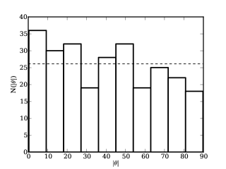
Figure 6.— Number of objects at angle $\theta$ where $\theta=0$ is aligned with the host major axis within radius of 20 $R_{\rm h}$ for hosts with axis ratio less than 0.6. The dashed line shows the average bin heights for a uniform distribution.

5. Joint Modeling of Satellite and Background Galaxy Populations

We have shown that the neighboring galaxies to the GOODS host galaxies exhibit non-trivial radial and angular distributions, and we now seek to model these distributions. We start in § 5.1 by defining the satellite model and the parameters we aim to constrain. In § 5.2 we discuss the background model and the priors we will be using. In § 5.3 we summarize our inference methodology, which is described in more detail in Appendix D. A summary of all model parameters and their priors is given in Table  1. Our implementation of the model and inference algorithm has been extensively tested by means of simulated data. To guide the reader, a schematic of a possible realization of our satellite plus background model is shown in Figure 7.

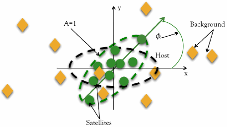
Figure 7.— Schematic illustrating a possible realization of our model.

5.1. Satellites

The scale-free nature of $\Lambda$CDM results motivates us to construct our model for the spatial distribution of the satellite number density as a function of corresponding host parameters. For simplicity, and owing to the relatively low signal-to-noise ratio of our measurement, we do not allow for intrinsic scatter in these scaling functions. Thus our inferences connecting host and satellite properties are averages for the entire population; individual systems will differ from the average.

We divide our discussion of our model for the satellite population into three subsections. We describe the probability of finding a satellite at a certain position in Subsection 5.1.1. We discuss choosing a region in which to search for satellites in order to normalize the spatial distribution in Subsection 5.1.2. Finally the probability of finding a certain number of objects around each host is discussed in Subsection 5.1.3.

5.1.1 Satellite Spatial Distribution

$\Lambda$CDM simulations indicate that the number density of satellites follows the mass density profile of their host galaxy (Kravtsov 2010). In turn, observations indicate that the three dimensional total mass density profile of elliptical galaxies can be approximated by a power law $\rho^{-\gamma^{\prime}}$ with $\gamma^{\prime}\approx 2$, (with $<$10% scatter) (e.g. Koopmans et al., 2009; Auger et al., 2010). The power law profile seems to extend as far as 100 $R_{\rm e}$ (e.g.  Gavazzi et al., 2007; Lagattuta et al., 2010) which corresponds to approximately 70 $R_{\rm h}$. We will thus model the radial distribution of satellites as a power law, with projected logarithmic slope $\gamma_{\rm p}=1-\gamma^{\prime}$.

We relate the angular light profile of the hosts to the mass profile following the results from the Sloan Lens ACS (SLACS) by Bolton et al. (2008, hereafter B08). B08 used gravitational lensing to study the relationship between the mass and light distributions of massive elliptical galaxies. B08 found that the major axes of the light profiles of the galaxies they studied were well aligned with the total central mass profiles and that the axis ratios of the light and mass profiles were the same within measurement errors; note that this agreement was established within the Einstein radii of the lensed galaxies, which corresponds to roughly $\sim$ 1″(see also Kochanek, 2002). The majority of our hosts are well represented by the properties of the SLACS lenses which are massive elliptical galaxies with stellar masses in the range $\sim 10^{10.5}$ to $10^{12}M\odot$ (Auger et al., 2009). This implies that we can expect the angular distribution of satellites to roughly follow that of host light and therefore that it is reasonable to construct a model of the satellite angular profile which is related to parameters which describe the host light angular profile.

We model the satellite distribution in an elliptical coordinate system described by an angle $\theta$ which is the same as the normal polar angle, and a radial coordinate $R^{\prime}$ related to Cartesian coordinates x, y by:

$$R^{\prime}=\sqrt{x^{2}+y^{2}/q^{2}}$$ (1)

Where $q$ is the ratio between minor and major axes of the elliptical coordinate system. The probability of finding a satellite on an elliptical contour within the area element $R^{\prime}dR^{\prime}d\theta^{\prime}$, goes as a power law with power $\gamma_{\rm p}$

$$P_{\rm s}(R^{\prime})R^{\prime}dR^{\prime}d\theta^{\prime}\propto(x^{2}+y^{2}/q^{2})^{\gamma_{\rm p}/2}dxdy.$$ (2)

Changing to polar coordinates gives

$$\begin{array}[]{l}P_{\rm s}(r,\theta|\phi,q,\gamma_{\rm p})\propto\\ \\ r^{\gamma_{\rm p}}[\cos^{2}{(\theta-\phi)}+1/q^{2}\sin^{2}{(\theta-\phi)}]^{\gamma_{\rm p}/2}rdrd\theta\end{array}$$ (3)

where we introduce $\phi$ to allow for some offset between the major axis of the satellite elliptical coordinate system and the major axis of the host galaxy; $\phi=0^{o}$ corresponds to parallel alignment, and $\phi=90^{o}$ corresponds to perpendicular alignment (see Figure 7). This is different from the coordinate $\theta$, which describes the offset between a particular object and the host major axis. We are only interested in the magnitude of the offset between the host light profile and the satellite population so we infer $|\phi|$, the absolute value of the offset of the distribution from the host major axis.

In general the offset $\phi$ in 3 dimensions is related to the 2D projected offset in a non-trivial way because of the random orientation of the host-satellite system in the plane perpendicular to the projection plane. However, for many interesting and plausible scenarios, the alignment in 3 dimensions relates in an obvious way to the observed, projected offset $\phi$. Namely, if the satellites are aligned with the host light distribution in 3D then the projection of the two systems will also appear aligned. Similarly, if the systems are anti-aligned, the satellites will appear perpendicular to the host in projection. Finally, if the satellites are oriented randomly with respect to the host in 3 dimensions, their projection will appear isotropic. Thus the projected relationship between the satellite spatial distribution and the host light profile contains relevant information about the 3D distribution.

We also aim to determine the connection between the ellipticity of the host light and that of the satellite distribution. For this purpose, we define the ellipticity to be:

$$\epsilon=\frac{1-q^{2}}{1+q^{2}},$$ (4)

We introduce a parameter $A$ to relate the ellipticity of the host profile, $\epsilon_{\rm h}$, to that of the satellite distribution, $\epsilon_{\rm s}$:

$$\epsilon_{\rm s}=\frac{\epsilon_{\rm h}A}{1+\epsilon_{\rm h}(A-1)}$$ (5)

We choose this parametrization because it returns valid ellipticities ($0<\epsilon<1$) for all values of $A>0$. This is convenient when exploring the $A$ parameter space with our MCMC code. The parameter $A$ can be understood as follows: when $A=0$, the satellite distribution is always round regardless of how flat the host distribution is; when $A=1$ the satellite distribution has the same flattening as the host distribution; and for values of $A>1$, the satellite distribution is more flat than the host light distribution. Note that formally $A$ goes from zero to infinity. As $A$ approaches infinity, the satellite distribution approaches $q=0$. We are interested in a qualitative characterization of the satellite flattening so we simplify our inference on $A$ by restricting our analysis to $0<A<2$, which will allow us to distinguish between isotropic and flattened satellite distributions without having to explore an unnecessarily large parameter space.

5.1.2 Spatial Normalization

We choose a maximum and minimum radius in which to search for satellites in order to normalize our distribution. These radii are determined by observational constraints. The inner radius is constrained to be $r_{\rm min}=1.5R_{\rm h}$ by our ability to accurately measure faint object magnitudes near the host (see Section 3.2). For the outer radius we choose $r_{\rm max}=45R_{\rm h}$ which corresponds to approximately 140 kpc. This choice is a compromise between studying an area large enough to find LMC/SMC equivalent objects (which are $\sim$ 60 kpc from the Milky Way), and keeping the area small enough to limit overlap between host galaxies and allowing us to reasonably apply a background prior determined by the entire field.

The normalized radial probability distribution is thus:

$$P_{\rm s}(r|\gamma_{\rm p})=\left(\frac{\gamma_{\rm p}+2}{r_{\rm max}^{\gamma_{\rm p}+2}-r_{\rm min}^{\gamma_{\rm p}+2}}\right)r^{\gamma_{\rm p}+1},$$ (6)

The normalization of the angular distribution is given by a generalized elliptical integral.

As discussed in Section 3.2, a few of our systems are not complete to the same inner radius due to issues with light modeling for highly flattened hosts. Furthermore, some of the regions far from the hosts are not complete to 45 $R_{\rm h}$ due to GOODS field edge effects. We discuss how we account for this incompleteness in Appendix C.

5.1.3 Number of satellites per host

Multiple dark matter simulations have found that the number of satellites with a given mass relative to the host mass is constant (Moore et al., 1999; Kravtsov et al., 2004; Gao et al., 2004). With this in mind, we model the number of satellites within a fixed magnitude range from the host as being drawn from a Poisson distribution with some constant mean $N_{\rm s}$.

It is important to keep in mind the following caveats. Due to baryonic physics, the observable properties of galaxies are not exactly scale invariant. In fact, the virial mass to light ratio is not a universal function and we expect it to vary for the host galaxies and satellites. This means that in a fixed magnitude range we are not actually probing a fixed virial mass range, but only a fixed range in luminosity ratio. However, it should be noted that our host galaxies are typically luminous enough (several $10^{10}L_{\odot}$) that their satellites are also significantly brighter than the typical Local Group dwarf galaxies where the M/L is believed to be much higher than in massive ellipticals. Thus our satellite mass range is better characterized by the relative luminosity between host and satellites than it would be for the Local Group.

Naturally, these assumptions will have no effect on our inference of the parameters of the satellite spatial distribution, provided that it is also independent of host galaxy luminosity within the spatial and mass ranges considered here.

5.2. Background/Foreground Objects

In addition to satellites, each of the host galaxies is surrounded in projection by background/foreground objects. We isolate the satellite signal by using the properties of the entire GOODS fields to provide a strong constraint on the background number density.

Galaxies tend to cluster on scales of order a typical galaxy virial radius, or $\sim 400$ kpc (e.g. Totsuji & Kihara, 1969; Peebles, 1974; Brainerd et al., 1995; Villumsen et al., 1997; Zehavi et al., 2002; Morganson & Blandford, 2009). This clustering is believed to be due to the accretion of matter along dark matter filaments (e.g. Benson, 2010, and references therein). Because of clustering, the density of objects tends to be higher in regions near bright galaxies and to have fluctuation amplitudes larger than Poissonian. Chen et al. (2006) tested a variety of methods for removing ‘interloper’ (background/foreground) contamination from their satellite signal using a set of $\Lambda$CDM simulations. Chen et al. (2006) found that simply estimating the number density of background objects by studying randomly selected regions in their field significantly underestimated the contamination from foreground/background objects that appeared near their hosts in projection. They found the most reliable estimate of the background was obtained by measuring the background in annuli centered on their hosts and just outside of the area in which they studied the satellite population. We adopt this method to build a prior on the background near the hosts. We study the background in annuli between 45 and 60 $R_{\rm h}$ (typically 140-180 kpc). We choose this distance range to ensure that we are not including satellites in our estimate, while still accurately characterizing the clustering of galaxies near the hosts. We find that the density of objects near the hosts with magnitudes within our detection range ($21<z_{850}<26.5$) is $\Sigma_{b,o}=125\pm 2$ arcmin^-2. As expected, this is higher than the average density of objects in the GOODS fields ($117\pm 0.6$) and has larger fluctuations than one would predict from Poisson noise.

Recall that we are studying objects brighter than a fixed magnitude contrast from the host magnitudes. This means that the number of objects we study around a given host is a fraction of the density of objects brighter than $z_{850}=26.5$. We correct for this around each of the hosts by representing the cumulative distribution function (CDF) of the background number counts by a power-law (e.g. Benitez et al., 2003)

$$N_{b}(<m_{\rm max})\propto 10^{\alpha_{\rm b}m_{\rm max}}$$ (7)

where $\alpha_{\rm b}$ is the slope of the background number counts. The maximum magnitude $m_{\rm max}$ for a particular host system is

$$m_{\rm max}=m_{\rm h}+\Delta m.$$ (8)

Thus for a given choice of $\Delta m$, the expected number density of background/foreground objects around the $j^{\rm th}$ host is

$$\Sigma_{\rm b,j}=\Sigma_{\rm b,o}10^{\alpha_{\rm b}(m_{\rm{h},j}+\Delta m-m_{\rm lim})}.$$ (9)

We measure the background slope to be $\alpha_{\rm b}=0.28\pm 0.01$ in the same annuli near the hosts in which we estimate the number density of the background.

5.3. Analysis

In the previous two subsections we constructed a model which describes the probability of a satellite or foreground/background object appearing a given distance from the host dependent on a choice of parameters. The parameters and their priors are listed in Table 1. Of key importance in our work is that our results are unbinned and analyzed in a fully Bayesian fashion. This means that for each parameter our result is a posterior probability distribution function (PDF) which describes the probability of a value of a parameter being true given our data (the likelihood) and our prior knowledge of the parameter (the prior).

In Appendix D we discuss the details of constructing the posterior probability function (Equation D4) which we use to study our parameter posterior PDFs. We compute the posterior PDFs using a Markov Chain Monte Carlo (MCMC) method. At least $10^{6}$ iterations per chain are performed in order to ensure convergence.

Table 1 Summary of model parameters

Parameter	Description	Prior
Satellite Model
Ns	Number of satellites per host	U(0,20)
$\gamma_{\rm p}$	Logarithmic slope of the satellite radial distribution	U(-5,0)
$A$	Flattening of the satellite number density distribution relative to host light flattening	U(0,2)
$|\phi|$	Offset between the major axis of satellite spatial distribution and the major axis of the host light profile.	U(0,$\pi/2$)
Background Model
$\Sigma_{\rm b,o}$	Number density of background objects with magnitudes between $21<z_{850}<26.5$	N(125,2)
$\alpha_{b}$	Logarithmic slope of the $z_{850}$ background number counts	N(0.28,0.01)

6. Results

We first discuss the results for the $\Delta m=5.5$ magnitude bin, which has the strongest signal. Table 2 contains a summary of the results of the inference. The posterior PDF for each variable is shown in Figure 8.

The first main result is the clear detection of a peak in the posterior PDF for $N_{\rm{s}}$ which is well removed from zero, indicating the detection of a population of satellites. Secondly, we find that the radial density profile of the satellite spatial distribution is consistent with isothermal ($\gamma_{\rm p}=-1$). Thirdly, the posterior PDF of $\phi$ is peaked at zero indicating that the satellite spatial distribution is preferentially aligned with that of the host. A KS test shows that a uniform distribution of angles is ruled out at more than a 99.99% CL.

Our results are inconclusive for the relationship between ellipticity of the satellite distribution and that of the host, described by the parameter $A$ (see Figure 8). This is not surprising as it takes a stronger signal to measure the ellipticity of a distribution than to measure its alignment. Our inability to infer $A$ is in part due to a degeneracy between $\phi$ and $A$. If $A$ is zero, all values of $\phi$ are equally probable. This can be seen in the contour plot shown in Figure 8. We show the effects of removing this degeneracy by performing a separate analysis on the $\Delta m=5.5$ data set, keeping $\phi$ fixed at zero. The results for this are shown in Figure 9. When $\phi$ is fixed at zero, the inference disfavors small values of A, which implies a disfavoring of satellite distributions that are rounder that that of the stars.

We also verified that our results are robust to small changes in limiting magnitude by repeating the analysis for $\Delta m=6.0$ and 5.0 magnitude bins. The $\Delta m=6.0$ bin clearly shows the presence of a satellite population, with the same isothermal slope observed for the $\Delta m=5.5$ range and the same angular alignment with the host major axis. The inferred satellite number is also consistent with the $\Delta m=5.5$ measurement, although there is a longer tail towards higher satellite numbers which might indicate a slightly higher number, as expected given the fainter limit. As discussed in Section 2, the number of hosts that are complete almost halves from $\Delta m=5.5$ to $6.0$ so the errors are larger for the $\Delta m=6.0$ inference overall. Interestingly, the analysis for $\Delta m=5.0$ did not conclusively detect a satellite population; the number of satellites is marginally more than 1-$\sigma$ greater than zero, and the uncertainties on the parameters describing the spatial distribution are similarly larger. This shows the crucial need for deep data in performing this kind of measurement. In all cases we recover our priors on the background parameters $\alpha_{b}$ and $\Sigma_{\rm b,o}$. We are not able to constrain these numbers further because in our model they are both degenerate with each other and with the number of satellites.

An important degeneracy is that between $N_{\rm s}$ and $\gamma_{\rm p}$. The inferred number of satellites is larger for a shallow radial profile and vice-versa. From theoretical and observational arguments (see the Introduction) we expect the radial profile to be close to isothermal and we expect alignment between host and satellites. It is thus instructive to repeat the analysis by fixing these parameters to their expected values $\gamma_{\rm p}=-1$ and $\phi=0$, thereby eliminating many of the degeneracies. The resulting posterior PDFs for $\Delta m=5.5$ are shown in Figure 10, while results for all magnitude ranges are summarized in Table 3.

As expected, fixing $\gamma_{\rm p}$ and $\phi$ lowers the uncertainty of our inference and the detection of satellites becomes more significant. It is also easier to compare the results across magnitude bins, and we see how the number of satellites indeed increases with $\Delta m$ and is consistent with a cumulative luminosity function going as $L^{-1}$ (i.e. similar to the cumulative mass function predicted from theory assuming $m\propto L^{-2}$), albeit with large errors. Furthermore, the posterior PDF of $A$ begins to disfavor a satellite population that is more isotropic than the stars in the galaxy. This is also broadly in line with expectations, as we expect that the distribution of stars has been made rounder than the host halo by dissipational processes.

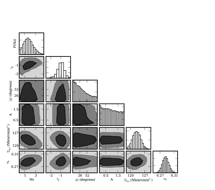
Figure 8.— Bivariate posterior PDFs for all model parameters for the $\Delta m=5.5$ data set. The dark and light contours contain regions of 68 and 95% of the probability respectively. The diagonal shows the marginalized PDF for each parameter.

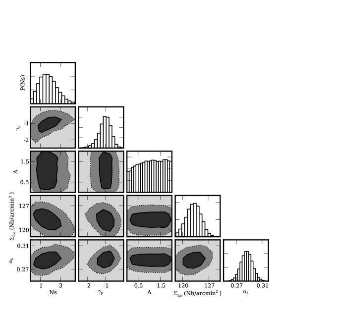
Figure 9.— Same as Figure 8, but with $\phi$ fixed at 0.

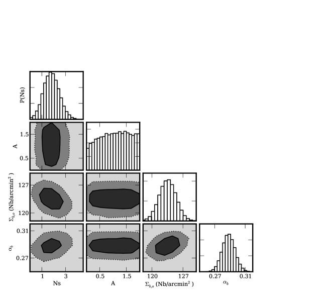
Figure 10.— Same as Figure 8, but with fixed $\phi=0$ and $\gamma_{\rm p}=-1$.

Table 2 Posterior Medians/Confidence Intervals

$\Delta m$	$\gamma_{\rm p}$	Ns	$|\phi|$	A	$\Sigma_{\rm b,o}$(N${}_{\rm b}/$arcmin2)	$\alpha_{b}$
			(68% confidence)
6.0	$-1.1^{+0.5}_{-0.6}$	$3^{+1}_{-1}$	$<44$	-	$123^{+2}_{-2}$	$0.283^{+0.009}_{-0.009}$
5.5	$-1.0^{+0.3}_{-0.4}$	$1.7^{+0.9}_{-0.8}$	$<42$	-	$123^{+2}_{-2}$	$0.286^{+0.009}_{-0.009}$
5.0	$-0.5^{+0.4}_{-0.8}$	$0.5^{+0.8}_{-0.4}$	$<56$	-	$124^{+2}_{-2}$	$0.282^{+0.009}_{-0.008}$

Table 3 Posterior Medians/Confidence Intervals with fixed parameters

Fixed parameter	$\Delta m$	$\gamma_{\rm p}$	Ns	A	$\Sigma_{\rm b,o}$(N${}_{\rm b}/$arcmin2)	$\alpha_{b}$
				(68% confidence)
$\phi=0$	5.5	$-1.0^{+0.3}_{-0.4}$	$1.7^{+1.0}_{-0.8}$	$>0.73$	$123^{+2}_{-2}$	$0.286^{+.009}_{-0.009}$
$\phi=0$, $\gamma_{\rm p}=-1$	6.0	-	$2^{+1}_{-1}$	$>0.83$	$124^{+2}_{-2}$	$0.285^{+0.009}_{-0.009}$
$\phi=0$, $\gamma_{\rm p}=-1$	5.5	-	$1.8^{+0.7}_{-0.6}$	$>0.72$	$124^{+2}_{-2}$	$0.288^{+0.008}_{-0.008}$
$\phi=0$, $\gamma_{\rm p}=-1$	5.0	-	$0.4^{+0.4}_{-0.3}$	$>0.73$	$124^{+2}_{-2}$	$0.281^{+0.008}_{-0.008}$

7. Discussion

This is the first measurement of the numbers and spatial distribution of faint satellites of early-type galaxies at intermediate redshift so it is useful to provide some context for our result. Our measurement of the radial slope of the satellite spatial distribution is consistent with an isothermal distribution, i.e. $\gamma_{\rm p}\approx-1$. This result is similar to that found in W10, and the radial distribution of satellites appears to be consistent with that of the total mass distribution measured in lensing studies (e.g., Koopmans et al., 2009; Auger et al., 2010). However, given the uncertainty on the inferred slope, the spatial distribution of satellites is also consistent with the NFW profile inferred by C08. In the radial range covered by our work ($\sim$5–140 kpc), an NFW profile is characterized by a radially averaged projected logarithmic slope of approximately $\gamma_{\rm p}\sim-1$, with large variations depending on host scale radius. More accurate measurements of the radial density profile of satellites are needed, in addition to a comparison of the radial profile around different host masses, in order to determine whether the distribution of satellites follows that of the total mass or that of the dark matter component.

The distribution of satellites is anisotropic and is preferentially aligned along the major axis of the host light profile. This host-satellite alignment is consistent with observations of host-satellite systems in SDSS (e.g. Brainerd, 2005). Furthermore, alignment is predicted by $\Lambda$CDM simulations which show satellites accreting anisotropically along filaments and appearing aligned with the major axis of the host mass profile (e.g., Aubert et al., 2004). Previous observations have established that the host light profile aligns with the host mass profile (B08), and our observation of the satellite-host light alignment therefore implies alignment between the satellite distribution and the host mass, in agreement with simulations. This alignment between host mass and satellite spatial distribution has important implications for the frequency of flux ratio anomalies, as we discuss below.

Although we do not expect the number of satellites of intermediate redshift elliptical galaxies to be exactly equal to that of galaxies at lower redshift due to baryonic processes and evolution, it is instructive to compare the GOODS satellites to other satellite populations. Figure 11 compares the cumulative luminosity function (CLF) of our satellites to the CLF of the Milky Way and Andromeda satellites (adopted from Tollerud et al., 2008), with one sigma uncertainties calculated from Gehrels (1986), and to the CLF of SDSS satellites of hosts with varying morphologies adopted from C08. Ideally, we would have also liked to compare our study to J10 which is one of the few studies of satellites of high redshift objects. However, the maximum value of $\Delta m$ in that survey was about 2.5 magnitudes which is too bright to be compared to our measurement in a meaningful way.

C08 measured the number of satellites and their radial profile between approximately 20 and 350 kpc. In order to compare our results appropriately, we use the C08 ‘interloper subtracted’ fit to a radial power law given in their Table 2 in order to extrapolate their measurement inward toward the host. We assume that the power law is constant in the inner regions and use a fiducial value of $R_{\rm h}\sim 3$ kpc to estimate the number of satellites C08 would have seen in the region that we studied (i.e., as close as 1.5 $R_{\rm h}$). The Milky Way CLF is complete in the same equivalent region as ours so we did not have to make any adjustments in order to compare our numbers. All three studies measured magnitudes in different filters; C08 used $r$ band magnitudes at an effective redshift of $z=0.1$, we use observed-frame $z_{850}$ magnitudes, and Milky Way measurements are in rest-frame $V$. However, the corrections required to convert from $r$ at redshift $\sim 0.1$ and observed $z_{850}$ at redshifts of $\sim 0.5$ into rest-frame V are negligible compared to the sizes of the bins of $\Delta m$ that we study, and we therefore do not include explicit $k$-corrections in our analysis. The three satellite CLFs are roughly consistent where the measurements overlap, given the relatively large error bars (Figure 11). It is worth noting that our GOODS satellite measurements have significantly smaller error bars than those for the Local Group by virtue of the large sample of hosts we study which allows us to reduce the sampling error. Furthermore, we are able to observe much fainter satellites than the SDSS study.

It is also instructive to compare our inferred satellite number to the number of minor mergers our hosts are expected to undergo in the time span we study. As many of our satellites are very near their host galaxies, we expect that some of them will be close to merging and that our estimate of the satellite number should account for the predicted minor merger rate in the mass range we study. The merger rate depends on the ratio between the host and satellite virial masses (e.g., Fakhouri et al., 2010). Our typical host has a stellar mass of M* $\sim 10^{10.5}$ M$\odot$ (see Figure 1). From abundance matching techniques (e.g., Behroozi et al., 2010), this corresponds to a halo mass of about $10^{12}~{}{\rm M}\odot$. In the luminosity range of our satellites the stellar mass to light ratio of the satellites should be approximately in the range 30-100% of that of the host galaxy (e.g., Kauffmann et al., 2003). Using this, the stellar mass of the satellites we study is in the range of $0.6-2\cdot 10^{8}$ M_⊙. This corresponds to virial masses of $\sim 2-8\cdot 10^{10}$ M_⊙, according to the best fit to Equation 21 in Behroozi et al. (2010). Thus the we can detect satellites with virial masses of order a percent of that of their hosts. This estimate is subject to large uncertainties, including those arising from tidal forces that tend to remove dark matter from satellites as they move closer to their host galaxy, thus reducing their virial mass. Using the best fit to Equation 1 in Fakhouri et al. (2010), we estimate that the majority of our hosts (60%) will undergo about 0.4-0.5 mergers (depending on the satellite stellar mass to luminosity fraction) between redshifts 0.1 and 0.8. It is reassuring that this number can be easily accounted for by our inferred satellite number. Of course, a quantitative comparison requires a detailed evaluation of the merging and visibility timescales, which is beyond the scope of this paper. However, we will re-visit this point in a future paper, as minor mergers have been suggested to play an important role in the evolution of early-type galaxies (e.g. Bundy et al., 2007; Boylan-Kolchin et al., 2008; Naab et al., 2009; Nipoti et al., 2009; Kaviraj et al., 2009; Hopkins et al., 2010; Kaviraj et al., 2011).

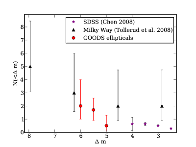
Figure 11.— Comparison of the measured number of GOODS satellites to those found for the Milky Way and SDSS galaxies.

Finally we discuss the effects our detected satellite population would have on flux ratio anomalies in quadruply-imaged strong gravitational lens systems. We limit our discussion here to order of magnitude estimates and general trends, leaving a rigorous quantitative analysis to a future paper.

Dalal & Kochanek (2002, hereafter D02) used the magnifications of images in five quad lenses to infer a mass profile for the lens galaxies. In order to reproduce the observed magnifications, D02 inferred the presence of a non-smooth component to the mass distribution with a mass fraction between 0.6 and 7 % near the lensed images. Mao et al. (2004) and more recently Xu et al. (2009, hereafter X09) used $\Lambda$CDM simulations to test whether dark substructure embedded within smooth halos could produce the flux ratio anomalies observed by D02. These studies estimated that the mass fraction of CDM substructure from their simulations would only be about 0.1 % near image positions, which is insufficient to produce the flux ratios studied by D02. The inclusion of globular cluster populations and baryonic processes does not change this result (Xu et al., 2010) and underscores the importance of constraining the satellite population through direct observations.

From our inference, a few percent of our hosts have a satellite within the annulus that would include the typical lens image positions studied by X09 (the Einstein radius is approximately 1″). We therefore find that the average mass fraction in this annulus is of order a few percent. Using the mass function ($dn/dm\propto m^{-1.9}$) described by X09, we estimate that the average satellite mass fraction they would have observed in our mass range is of order a percent, which is consistent with our result. It is worth considering the possibility that the presence of a few relatively massive satellites may increase the lensing cross-section significantly so that any attempt to measure the satellite mass function using gravitational lenses would be automatically biased towards very high mass fractions near the lens Einstein radius; we will explore this possibility in more detail in paper III.

It is interesting to note that, although our typical hosts have similar halo masses to those studied in X09, the most massive subhalo X09 observed in any of their simulations has a virial mass of $\sim 10^{10}~{}{\rm M}~{}\odot$, which is on the very low mass end of the subhalos studied in this work. Our simple extension of the virial to stellar mass relationship led us to estimate that our hosts will have on average more than one halo at least this massive even assuming that the mass to light ratio of our satellites is only a few percent of that of the host halo. This discrepancy may be due to the fact that our mass estimate is very approximate and, as already discussed, may not be appropriate for systems undergoing strong interactions such as tidal stripping. On the other hand, the difference in estimated satellite masses may indicate the importance of baryonic condensation in preserving the mass in subhalos during accretion (see e.g., Weinberg et al., 2008; Romano-Díaz et al., 2009).

Our observation that satellites appear preferentially along the host major axis may offer an additional route to reduce or eliminate the apparent discrepancy in the satellite mass fraction as inferred by flux ratio anomalies. As pointed out by Zentner (2006), an anisotropic satellite distribution can increase the effective projected mass of the host ‘felt’ by a lensed image by as much as a factor of six. Thus, the mass associated with our observed luminous satellites could in principle be sufficient to explain the anomalies detected by D02.

Our satellites are much fainter than a typical lensed quasar image and thus would be easily obscured in any of these lensing studies. Our result highlights the importance of studying the satellite population in non-lens systems in conjunction with the analysis of perturbations in lens systems in order to attain an understanding of the mass and luminosity functions of satellites.

To conclude, it is important to point out that the largest discrepancies between the luminosity and mass function are seen for even fainter satellites than the ones probed by this study (Kravtsov, 2010). It is thus desirable to push the analysis of both the luminosity and the mass function of satellites to even smaller fractions of the host galaxy properties.

8. Summary

We use an advanced host light subtraction method to study the spatial distribution of faint galaxies around 127 early-type galaxies in the GOODS fields between redshifts 0.1 and 0.8. We employ a self-consistent model in the framework of Bayesian inference to disentangle the satellite population from background/foreground galaxies. Exploiting the depth and resolution of the HST images, we detect satellites up to 5.5 magnitudes fainter than the host galaxy and as close as 0$\farcs$5/2.5 kpc to the host. Our main results can be summarized as follows:

1. Intermediate redshift, massive, early-type galaxies have on average $1.7^{+0.9}_{-0.8}$ satellites within our luminosity ratio limit. This is consistent with the number of satellites observed in the Milky Way.

2. The number density of satellites follows an approximately isothermal radial power law profile $P(r)\propto r^{\gamma_{\rm p}}$ with $\gamma_{\rm p}=-1.0^{+0.3}_{-0.4}$.

3. The satellites are preferentially aligned along the major axis of the host light profile with $|\phi|<42^{o}$ at the 68% confidence level.

4. When the offset $\phi$ between the satellite population and host light profile is fixed at 0 degrees, the satellite distribution is inferred to be preferentially more elongated than the distribution of host galaxy light.

5. When the satellite number density profile is assumed to be isothermal, the average number of satellites is inferred to be 1.8${}^{+0.7}_{-0.6}$.

Appendix A Host Galaxy Light Subtraction

As we showed in Section 3, the detectability of satellite galaxies is quite sensitive to the presence of light from the much brighter host galaxy. In this appendix we give more details on how the light from the host galaxy was subtracted in order to allow the faint satellites to be detected. Host galaxy surface brightness modeling is a two step process. In the first step, we identify and mask all objects other than the host in the region in which we want to model host galaxy light. This ensures that our host model does not attempt to fit the light of nearby objects. Once the objects are identified and the mask is created, in the second step we model the host galaxy surface brightness in 2D using the unmasked parts of the image, interpolate over the masked parts, and subtract this model from our original image.

A.1. Masking

The masking is done automatically using the segmentation map produced by an initial SExtractor run, with parameters tuned to optimize the detection of small faint objects in the presence of the host light. This optimization was performed by simulating faint companion objects at varying positions around our hosts. We found that using the GOODS SExtractor parameters at this stage gave unsatisfactory results, in that objects we simulated near the hosts were not being masked. We found that, in order to properly account for both faint point sources near our hosts and diffuse sources further from our hosts, we needed to use a superposition of masks created with two different sets of SExtractor parameters. These parameters are listed in Table 4. With this masking routine, we were able to accurately recover magnitude 27 point sources as close as 1.5 $R_{\rm h}$ (typically $\sim$ 0$\farcs$9) from our host galaxy centroids.

Table 4 SExtractor Parameters

Parameter	Value
	Large Object Mask	Point Object Mask	Final Photometry
DETECT_MINAREA	10	5	–
DEBLEND_NTHRESH	64	–	–
DEBLEND_MINCONT	0.001	–	–
DETECT_THRESH	–	2.5	–
ANALYSIS_THRESH	–	2.5	–
FILTER_NAME	–	gauss_2.0_3x3.conv	–
BACK_TYPE	MANUAL	MANUAL	MANUAL
BACK_VALUE	0.0	0.0	0.0

Note. — Parameters not listed, or marked as “–”, are those used by the GOODS team and can be found at. http://archive.stsci.edu/pub/hlsp/goods/catalog_r2

A.2. B-spline model subtraction

In Figure 2 we show some representative examples of our host galaxy light subtraction process. Some of our hosts are very elongated or show disk-like features. The surface brightness distribution of these objects is more difficult to model and tends to leave residuals at larger radii than the rounder hosts. Residuals are easily identifiable because of the symmetric pattern and distinct elongated shape that they appear in (see, e.g., the residuals of the upper right host in Figure 2). We deal with this small number ($\sim 20$) of more disky/extended sources in two ways. The first way is to increase the amount of flexibility in the B-spline fit, increasing the number of multipoles fitted in each of our spline rings around the ellipse. The second thing we do is to exclude a larger inner region from our analysis to ensure we are not identifying any residuals as objects.

Appendix B Source Extractor Parameters and Photometry Comparison

After subtracting the main galaxy light out of the image we run SExtractor on the residual image to identify the remaining objects. In this step we modify our SExtractor parameters by increasing the deblending threshold in order to match the parameters used when making the GOODS catalogs. A full list of our SExtractor parameters is listed in Table 4.

Even after matching the deblending parameters, there are two minor differences between our final SExtractor parameters and GOODS SExtractor parameters. The first is that GOODS estimates the background by measuring the noise in an annulus with 100 pixel (3″) width around each object. This method of background subtraction is not optimal for our measurement because we are focusing on a relatively small area (typical image size was $\sim 200$x$200$ pixels), within which we expect to have a relatively high object density. Instead, we estimate the background by calculating the 3 $\sigma$ clipped mean within our image. Furthermore, the GOODS team made modifications to SExtractor that changed the deblending process slightly.

We compare the MAG_AUTO output from SExtractor for the two methods in a 4 arcmin² cutout from the GOODS field in order to study the effects of the different background subtraction and deblending (see Figure 12). Using our parameters, we identify 484 objects with MAG_AUTO$<$26.5. Of these, 22 objects do not have a center within 0$\farcs$3 of an object in the GOODS catalog. The major outliers in the MAG_AUTO comparison are all in areas of high object density and thus most likely due to differences in deblending. The mean difference (not including major outliers) in the MAG_AUTO estimate is $(-1.9\pm 6.0)\cdot 10^{-3}$.

Figure 12.— Comparison of our photometry with GOODS in a 4 arcmin² field cutout with no host galaxy subtraction.

Appendix C Completeness

In Section 5 we discuss our model for the spatial distribution of satellites which we can use to calculate the probability that there are a certain number of objects $\hat{N}$ within $1.5<r/R_{h}<45$, with positions $\bm{x}$. Before comparing a particular model prediction to the data it is necessary to account for observational limitations such as field edge effects. In this section we explain how we account for these observational limitations when inferring our model parameters.

Following Kelly (2007), we define a completeness function, $P(I|\bm{x})$, which describes the probability of observing an object at position $\bm{x}$, where $I=1$ indicates an object is detected and $I=0$ indicates a non-detection. Note that because we have chosen to study only magnitude ranges in which we are complete, our completeness function will only depend on position in a given field. As discussed in Appendix A, we measure our completeness near the host galaxy by placing simulated objects around the host and calculating our recovery rate and the accuracy of our photometry as a function of position. Far from the host, we estimate our completeness in annuli to account for field edge effects. To simplify this analysis, we ignore regions of partial completeness so that a region in the field is either 100% complete or 0% complete.

Taking completeness into account, the likelihood of detecting $N^{\rm obs}$ total objects (satellites and background),with positions $\{\bm{x}\}$, given model parameters $\bm{\theta}$, becomes

$${\rm Pr}(N^{\rm obs},\{\bm{x}\}|\bm{\theta})={\rm Pr}(I|\{\bm{x}\}){\rm Pr}(\hat{N},\{\bm{x}\}|\bm{\theta})$$ (C1)

Our fields have varying sizes but the model parameter $\hat{N}$ gives the number of objects we expect to find in an ideal field where we have 100% completeness between $1.5$ and $45$ $R_{\rm h}$. As discussed above, some of our host systems have restricted areas, between $r_{mn}$ and $r_{mx}$, where the total area is smaller than in the ideal case. In these cases we must scale the model prediction by the probability of finding the object in the reduced area compared to the probability of finding the object in the ideal area, and we therefore define an updated prediction for the number of objects $\hat{N}^{\prime}$ given by

$$\hat{N}^{\prime}=\hat{N}\frac{\int_{r_{mn}}^{r_{mx}}{\rm Pr}(\bm{x}^{\prime}|\bm{\theta})d\bm{x}^{\prime}}{\int_{1.5}^{45}{\rm Pr}(\bm{x}^{\prime}|\bm{\theta})d\bm{x}^{\prime}}$$ (C2)

Note that $\hat{N}$ is a smooth model prediction of the number of true objects in a field. In order to properly account for the fact that the true number of objects in a field is discrete, we must introduce a Poisson probability, which relates the “true” discrete number of objects to the model number of objects. The likelihood that we observe $N^{\rm obs}$ objects at positions $\bm{x}$ given our model parameters, is a product over the likelihood of each of those positions being true given our model parameters

$${\rm Pr}(\{\bm{x}\}|\bm{\theta})=\prod_{i}^{N^{\rm obs}}{\rm Pr}(\bm{x}_{i}|\bm{\theta})$$ (C3)

Thus the probability that we observe $N^{\rm obs}$ given a set of model parameters, taking into account varying total areas of completeness, is given by:

$${\rm Pr}(N^{\rm obs},\{\bm{x}\}|\bm{\theta})={\rm Pr}(N^{\rm obs}|\hat{N}^{\prime})\prod_{i}^{N^{\rm obs}}{\rm Pr}(\bm{x}_{i}|\bm{\theta}).$$ (C4)

Properly, we should also include a term which accounts for the probability of not observing $N-N^{\rm obs}$ objects. However, in our case, the region of parameter space we exclude due to observational limitations is always much smaller than the region we do study, and thus the number of objects our model predicts that we expect to observe is much larger than the number that we cannot observe. Therefore, for simplicity, we do not include this term in our analysis.

Appendix D Inference methodology

In this section we discuss in detail how we characterize the posterior PDFs for our satellite model parameters $\bm{\theta}_{\rm s}=\{N_{s},\gamma_{\rm p},A,\phi\}$, and our background model parameters $\bm{\theta}_{\rm b}=\{\Sigma_{\rm b,o},\alpha_{b}\}$. We present a top-down description of our model in which we start with the posterior PDF we would like to obtain and break it apart to show where we have inserted different pieces of information.

Our final data set, $\bm{D}$, is composed of a set of measurements for all of our host-field systems, $\bm{D}=\{\bm{D}_{1},\bm{D}_{2},...,\bm{D}_{N_{h}}\}$ Where $\bm{D}_{j}=\{\bm{h}_{j},\bm{d}_{j}\}$, and $\bm{h}_{j}$ is the set of measurements of the magnitude, axis ratio and RMS of the $j^{th}$ host light profile, and $\bm{d}_{j}=\left[N^{\rm obs}_{j},\{(\bm{x}_{1}),(\bm{x}_{2}),...(\bm{x}_{N^{\rm obs}_{j}})\}\right]$ is the number of objects observed around the $j^{th}$ host and their positions. Using Bayes’ theorem we can express the probability of a set of model parameters being true given the data by:

$${\rm Pr}(\bm{\theta}|\bm{D})\propto{\rm Pr}(\bm{D}|\bm{\theta}){\rm Pr}(\bm{\theta})$$ (D1)

In the above equation the term ${\rm Pr}(\bm{D}|\bm{\theta})$ is the likelihood of the data being true given a set of model parameters and ${\rm Pr}(\bm{\theta})$ is the prior information we have about the model parameters. Our model parameters and their priors are listed in Table 1.

The first term on the right of Equation D1 is a product of likelihoods for individual host systems:

$${\rm Pr}(\bm{D}|\bm{\theta})=\prod_{j}^{N_{\rm h}}{\rm Pr}(\bm{d}_{j}|\bm{\theta},\bm{h}_{j})$$ (D2)

Notice that in our model, the measurements of the host light profile are treated as model parameters which we assume are known exactly. This is because we have constructed our model such that its parameters do not predict the properties of the host light profile.

Equation D2 is itself composed of a product of the likelihood of measuring $N^{\rm obs}_{j}$ objects around each host times the probability for measuring each object position,

$${\rm Pr}(\bm{d}_{j}|\bm{\theta},\bm{h}_{j})={\rm Pr}(N^{\rm obs}_{j}|\bm{\theta})\prod_{i}{\rm Pr}(\bm{x}_{i}|\bm{\theta},\bm{h}_{j})$$ (D3)

Recall that in Section 5 we built a model that was composed of separate contributions from a satellite and background population. This means that the probability of finding any object at a given location is the sum of the probability of finding a background object at that location with the probability of a finding a satellite at that location:

$${\rm Pr}(\bm{d}_{j}|\bm{\theta},\bm{h}_{j})={\rm Pr}(N^{\rm obs}|\bm{\theta})\prod_{i}{\rm Pr}(\bm{x}_{i}|\bm{\theta},\bm{h}_{j},S){\rm Pr}(S|\bm{\theta},\bm{h}_{j})+{\rm Pr}(\bm{x}_{i}|\bm{\theta},\bm{h}_{j},B){\rm Pr}(B|\bm{\theta},\bm{h}_{j})$$ (D4)

The term ${\rm Pr}(\bm{x}_{i}|\bm{\theta},\bm{h}_{j},S)$ is the probability of finding a satellite at a certain position (given by Equation 3) and ${\rm Pr}(\bm{x}_{i}|\bm{\theta},\bm{h}_{j},B)$ is the probability of finding a background/foreground object at a certain position (which is uniform). The term ${\rm Pr}(S|\bm{\theta},\bm{h}_{j})$ is the probability of an object being a satellite given only the model parameters,

$${\rm Pr}(S|\bm{\theta},\bm{h}_{j})=\frac{N_{s}}{N_{s}+N_{b}}$$ (D5)

and ${\rm Pr}(B|\bm{\theta},\bm{h}_{j})$ is defined in an analogous way for the line-of-sight interlopers. The functions that determine $N_{s}$ and $N_{b}$ in terms of model parameters are discussed in Section 5.

References

- Agustsson & Brainerd (2010) Agustsson, I., & Brainerd, T. G. 2010, ApJ, 709, 1321
- Aubert et al. (2004) Aubert, D., Pichon, C., & Colombi, S. 2004, MNRAS, 352, 376
- Auger et al. (2009) Auger, M. W., Treu, T., Bolton, A. S., Gavazzi, R., Koopmans, L. V. E., Marshall, P. J., Bundy, K., & Moustakas, L. A. 2009, ApJ, 705, 1099
- Auger et al. (2010) Auger, M. W., Treu, T., Bolton, A. S., Gavazzi, R., Koopmans, L. V. E., Marshall, P. J., Moustakas, L. A., & Burles, S. 2010, ArXiv e-prints
- Behroozi et al. (2010) Behroozi, P. S., Conroy, C., & Wechsler, R. H. 2010, ApJ, 717, 379
- Bell et al. (2006) Bell, E. F., Phleps, S., Somerville, R. S., Wolf, C., Borch, A., & Meisenheimer, K. 2006, ApJ, 652, 270
- Benitez et al. (2003) Benitez, N., Ford, H., Bouwens, R., Menanteau, F., Blakeslee, J., Gronwall, C., Illingworth, G., Meurer, G., Broadhurst, T. J., Clampin, M., Franx, M., Hartig, G., Magee, D., Sirianni, M., Ardila, D. R., Bartko, F., Brown, R. A., Burrows, C. J., Cheng, E. S., Cross, N. J. G., Feldman, P. D., Golimowski, D. A., Infante, L., Kimble, R. A., Krist, J. E., Lesser, M. P., Levay, Z., Martel, A. R., Miley, G. K., Postman, M., Rosati, P., Sparks, W. B., Tran, H. D., Tsvetanov, Z. I., White, R. L., & Zheng, W. 2003, ArXiv Astrophysics e-prints
- Benson (2010) Benson, A. J. 2010, Phys. Rep., 495, 33
- Bertin & Arnouts (1996) Bertin, E., & Arnouts, S. 1996, A&AS, 117, 393
- Blumenthal et al. (1986) Blumenthal, G. R., Faber, S. M., Flores, R., & Primack, J. R. 1986, ApJ, 301, 27
- Bolton et al. (2005) Bolton, A. S., Burles, S., Koopmans, L. V. E., Treu, T., & Moustakas, L. A. 2005, ApJ, 624, L21
- Bolton et al. (2006) —. 2006, ApJ, 638, 703
- Bolton et al. (2008) Bolton, A. S., Treu, T., Koopmans, L. V. E., Gavazzi, R., Moustakas, L. A., Burles, S., Schlegel, D. J., & Wayth, R. 2008, ArXiv e-prints, 805
- Boylan-Kolchin et al. (2008) Boylan-Kolchin, M., Ma, C., & Quataert, E. 2008, MNRAS, 383, 93
- Brainerd (2005) Brainerd, T. G. 2005, ApJL, 628, L101
- Brainerd et al. (1995) Brainerd, T. G., Smail, I., & Mould, J. 1995, MNRAS, 275, 781
- Bundy et al. (2005) Bundy, K., Ellis, R. S., & Conselice, C. J. 2005, VizieR Online Data Catalog, 7246, 0
- Bundy et al. (2009) Bundy, K., Fukugita, M., Ellis, R. S., Targett, T. A., Belli, S., & Kodama, T. 2009, ApJ, 697, 1369
- Bundy et al. (2007) Bundy, K., Treu, T., & Ellis, R. S. 2007, ApJL, 665, L5
- Chen (2008) Chen, J. 2008, A&A, 484, 347
- Chen et al. (2006) Chen, J., Kravtsov, A. V., Prada, F., Sheldon, E. S., Klypin, A. A., Blanton, M. R., Brinkmann, J., & Thakar, A. R. 2006, ApJ, 647, 86
- Cohn et al. (2001) Cohn, J. D., Kochanek, C. S., McLeod, B. A., & Keeton, C. R. 2001, ApJ, 554, 1216
- Colín et al. (2000) Colín, P., Avila-Reese, V., & Valenzuela, O. 2000, ApJ, 542, 622
- Dalal & Kochanek (2002) Dalal, N., & Kochanek, C. S. 2002, ApJ, 572, 25
- de Rijcke et al. (2009) de Rijcke, S., Penny, S. J., Conselice, C. J., Valcke, S., & Held, E. V. 2009, MNRAS, 393, 798
- Fakhouri et al. (2010) Fakhouri, O., Ma, C., & Boylan-Kolchin, M. 2010, MNRAS, 406, 2267
- Faltenbacher et al. (2008) Faltenbacher, A., Jing, Y. P., Li, C., Mao, S., Mo, H. J., Pasquali, A., & van den Bosch, F. C. 2008, ApJ, 675, 146
- Faltenbacher et al. (2007) Faltenbacher, A., Li, C., Mao, S., van den Bosch, F. C., Yang, X., Jing, Y. P., Pasquali, A., & Mo, H. J. 2007, ApJL, 662, L71
- Gao et al. (2004) Gao, L., White, S. D. M., Jenkins, A., Stoehr, F., & Springel, V. 2004, MNRAS, 355, 819
- Gavazzi et al. (2007) Gavazzi, R., Treu, T., Rhodes, J. D., Koopmans, L. V., Bolton, A. S., Burles, S., Massey, R., & Moustakas, L. A. 2007, ArXiv Astrophysics e-prints
- Gehrels (1986) Gehrels, N. 1986, ApJ, 303, 336
- Giavalisco et al. (2004) Giavalisco, M., et al. 2004, ApJL, 600, L93
- Gnedin (2000) Gnedin, N. Y. 2000, ApJL, 535, L75
- Gnedin et al. (2004) Gnedin, O. Y., Kravtsov, A. V., Klypin, A. A., & Nagai, D. 2004, ApJ, 616, 16
- Hopkins et al. (2010) Hopkins, P. F., Bundy, K., Croton, D., Hernquist, L., Keres, D., Khochfar, S., Stewart, K., Wetzel, A., & Younger, J. D. 2010, ApJ, 715, 202
- Jackson et al. (2010) Jackson, N., Bryan, S. E., Mao, S., & Li, C. 2010, MNRAS, 403, 826
- Kamionkowski & Liddle (2000) Kamionkowski, M., & Liddle, A. R. 2000, Physical Review Letters, 84, 4525
- Kauffmann et al. (2003) Kauffmann, G., Heckman, T. M., White, S. D. M., Charlot, S., Tremonti, C., Brinchmann, J., Bruzual, G., Peng, E. W., Seibert, M., Bernardi, M., Blanton, M., Brinkmann, J., Castander, F., Csábai, I., Fukugita, M., Ivezic, Z., Munn, J. A., Nichol, R. C., Padmanabhan, N., Thakar, A. R., Weinberg, D. H., & York, D. 2003, MNRAS, 341, 33
- Kaufmann et al. (2008) Kaufmann, T., Bullock, J. S., Maller, A., & Fang, T. 2008, in American Institute of Physics Conference Series, Vol. 1035, The Evolution of Galaxies Through the Neutral Hydrogen Window, ed. R. Minchin & E. Momjian, 147–150
- Kaviraj et al. (2009) Kaviraj, S., Peirani, S., Khochfar, S., Silk, J., & Kay, S. 2009, MNRAS, 394, 1713
- Kaviraj et al. (2011) Kaviraj, S., Tan, K., Ellis, R. S., & Silk, J. 2011, MNRAS, 84
- Kelly (2007) Kelly, B. C. 2007, ApJ, 665, 1489
- Klypin et al. (1999) Klypin, A., Kravtsov, A. V., Valenzuela, O., & Prada, F. 1999, ApJ, 522, 82
- Knebe et al. (2004) Knebe, A., Gill, S. P. D., Gibson, B. K., Lewis, G. F., Ibata, R. A., & Dopita, M. A. 2004, ApJ, 603, 7
- Kochanek (2002) Kochanek, C. S. 2002, in The Shapes of Galaxies and their Dark, ed. P. Natarajan, 62–+
- Koopmans (2005) Koopmans, L. V. E. 2005, MNRAS, 363, 1136
- Koopmans et al. (2009) Koopmans, L. V. E., Bolton, A., Treu, T., Czoske, O., Auger, M. W., Barnabè, M., Vegetti, S., Gavazzi, R., Moustakas, L. A., & Burles, S. 2009, ApJL, 703, L51
- Koopmans et al. (2006) Koopmans, L. V. E., Treu, T., Bolton, A. S., Burles, S., & Moustakas, L. A. 2006, ApJ, 649, 599
- Kravtsov (2010) Kravtsov, A. 2010, Advances in Astronomy, 2010
- Kravtsov et al. (2004) Kravtsov, A. V., Gnedin, O. Y., & Klypin, A. A. 2004, ApJ, 609, 482
- Lagattuta et al. (2010) Lagattuta, D. J., Fassnacht, C. D., Auger, M. W., Marshall, P. J., Bradač, M., Treu, T., Gavazzi, R., Schrabback, T., Faure, C., & Anguita, T. 2010, ApJ, 716, 1579
- Le Fèvre et al. (2000) Le Fèvre, O., Abraham, R., Lilly, S. J., Ellis, R. S., Brinchmann, J., Schade, D., Tresse, L., Colless, M., Crampton, D., Glazebrook, K., Hammer, F., & Broadhurst, T. 2000, MNRAS, 311, 565
- MacLeod et al. (2009) MacLeod, C. L., Kochanek, C. S., & Agol, E. 2009, ApJ, 699, 1578
- Mao et al. (2004) Mao, S., Jing, Y., Ostriker, J. P., & Weller, J. 2004, ApJL, 604, L5
- McKean et al. (2005) McKean, J. P., Browne, I. W. A., Jackson, N. J., Koopmans, L. V. E., Norbury, M. A., Treu, T., York, T. D., Biggs, A. D., Blandford, R. D., de Bruyn, A. G., Fassnacht, C. D., Mao, S., Myers, S. T., Pearson, T. J., Phillips, P. M., Readhead, A. C. S., Rusin, D., & Wilkinson, P. N. 2005, MNRAS, 356, 1009
- Metz et al. (2009) Metz, M., Kroupa, P., & Jerjen, H. 2009, MNRAS, 394, 2223
- Moore et al. (1999) Moore, B., Ghigna, S., Governato, F., Lake, G., Quinn, T., Stadel, J., & Tozzi, P. 1999, ApJL, 524, L19
- Morganson & Blandford (2009) Morganson, E., & Blandford, R. 2009, MNRAS, 398, 769
- Naab et al. (2009) Naab, T., Johansson, P. H., & Ostriker, J. P. 2009, ApJL, 699, L178
- Navarro et al. (1996) Navarro, J. F., Frenk, C. S., & White, S. D. M. 1996, ApJ, 462, 563
- Nipoti et al. (2009) Nipoti, C., Treu, T., Auger, M. W., & Bolton, A. S. 2009, ApJL, 706, L86
- Oguri & Marshall (2010) Oguri, M., & Marshall, P. J. 2010, MNRAS, 587
- Oke (1974) Oke, J. B. 1974, ApJS, 27, 21
- Patton & Atfield (2008) Patton, D. R., & Atfield, J. E. 2008, ApJ, 685, 235
- Peebles (1974) Peebles, P. J. E. 1974, A&A, 32, 197
- Robaina et al. (2010) Robaina, A. R., Bell, E. F., van der Wel, A., Somerville, R. S., Skelton, R. E., McIntosh, D. H., Meisenheimer, K., & Wolf, C. 2010, ApJ, 719, 844
- Romano-Díaz et al. (2009) Romano-Díaz, E., Shlosman, I., Heller, C., & Hoffman, Y. 2009, ApJ, 702, 1250
- Scoville et al. (2007) Scoville, N., Abraham, R. G., Aussel, H., Barnes, J. E., Benson, A., Blain, A. W., Calzetti, D., Comastri, A., Capak, P., Carilli, C., Carlstrom, J. E., Carollo, C. M., Colbert, J., Daddi, E., Ellis, R. S., Elvis, M., Ewald, S. P., Fall, M., Franceschini, A., Giavalisco, M., Green, W., Griffiths, R. E., Guzzo, L., Hasinger, G., Impey, C., Kneib, J., Koda, J., Koekemoer, A., Lefevre, O., Lilly, S., Liu, C. T., McCracken, H. J., Massey, R., Mellier, Y., Miyazaki, S., Mobasher, B., Mould, J., Norman, C., Refregier, A., Renzini, A., Rhodes, J., Rich, M., Sanders, D. B., Schiminovich, D., Schinnerer, E., Scodeggio, M., Sheth, K., Shopbell, P. L., Taniguchi, Y., Tyson, N. D., Urry, C. M., Van Waerbeke, L., Vettolani, P., White, S. D. M., & Yan, L. 2007, ApJS, 172, 38
- Springel (2010) Springel, V. 2010, ARAA, 48, 391
- Strigari et al. (2007) Strigari, L. E., Bullock, J. S., Kaplinghat, M., Diemand, J., Kuhlen, M., & Madau, P. 2007, ApJ, 669, 676
- Thoul & Weinberg (1996) Thoul, A. A., & Weinberg, D. H. 1996, ApJ, 465, 608
- Tollerud et al. (2008) Tollerud, E. J., Bullock, J. S., Strigari, L. E., & Willman, B. 2008, ApJ, 688, 277
- Totsuji & Kihara (1969) Totsuji, H., & Kihara, T. 1969, PASJ, 21, 221
- Treu (2010) Treu, T. 2010, ARAA, 48, 87
- Treu et al. (2005) Treu, T., Ellis, R. S., Liao, T. X., & van Dokkum, P. G. 2005, ApJL, 622, L5
- Treu & Koopmans (2004) Treu, T., & Koopmans, L. V. E. 2004, ApJ, 611, 739
- Trujillo et al. (2006) Trujillo, I., et al. 2006, ApJ, 650, 18
- Vegetti et al. (2009) Vegetti, S., Koopmans, L. V. E., Bolton, A., Treu, T., & Gavazzi, R. 2009, ArXiv e-prints
- Vegetti et al. (2010) —. 2010, MNRAS, 408, 1969
- Villumsen et al. (1997) Villumsen, J. V., Freudling, W., & da Costa, L. N. 1997, ApJ, 481, 578
- Wang et al. (2008) Wang, Y., Yang, X., Mo, H. J., Li, C., van den Bosch, F. C., Fan, Z., & Chen, X. 2008, MNRAS, 385, 1511
- Watson et al. (2010) Watson, D. F., Berlind, A. A., McBride, C. K., & Masjedi, M. 2010, ApJ, 709, 115
- Weinberg et al. (2008) Weinberg, D. H., Colombi, S., Davé, R., & Katz, N. 2008, ApJ, 678, 6
- Williams et al. (2010) Williams, R. J., Quadri, R. F., Franx, M., van Dokkum, P., Toft, S., Kriek, M., & Labbé, I. 2010, ApJ, 713, 738
- Wolf et al. (2004) Wolf, C., Meisenheimer, K., Kleinheinrich, M., Borch, A., Dye, S., Gray, M., Wisotzki, L., Bell, E. F., Rix, H., Cimatti, A., Hasinger, G., & Szokoly, G. 2004, A&A, 421, 913
- Xu et al. (2010) Xu, D. D., Mao, S., Cooper, A. P., Wang, J., Gao, L., Frenk, C. S., & Springel, V. 2010, MNRAS, 408, 1721
- Xu et al. (2009) Xu, D. D., Mao, S., Wang, J., Springel, V., Gao, L., White, S. D. M., Frenk, C. S., Jenkins, A., Li, G., & Navarro, J. F. 2009, MNRAS, 398, 1235
- Yang et al. (2006) Yang, X., van den Bosch, F. C., Mo, H. J., Mao, S., Kang, X., Weinmann, S. M., Guo, Y., & Jing, Y. P. 2006, MNRAS, 369, 1293
- Zehavi et al. (2002) Zehavi, I., Blanton, M. R., Frieman, J. A., Weinberg, D. H., Mo, H. J., Strauss, M. A., Anderson, S. F., Annis, J., Bahcall, N. A., Bernardi, M., Briggs, J. W., Brinkmann, J., Burles, S., Carey, L., Castander, F. J., Connolly, A. J., Csabai, I., Dalcanton, J. J., Dodelson, S., Doi, M., Eisenstein, D., Evans, M. L., Finkbeiner, D. P., Friedman, S., Fukugita, M., Gunn, J. E., Hennessy, G. S., Hindsley, R. B., Ivezić, Ž., Kent, S., Knapp, G. R., Kron, R., Kunszt, P., Lamb, D. Q., Leger, R. F., Long, D. C., Loveday, J., Lupton, R. H., McKay, T., Meiksin, A., Merrelli, A., Munn, J. A., Narayanan, V., Newcomb, M., Nichol, R. C., Owen, R., Peoples, J., Pope, A., Rockosi, C. M., Schlegel, D., Schneider, D. P., Scoccimarro, R., Sheth, R. K., Siegmund, W., Smee, S., Snir, Y., Stebbins, A., Stoughton, C., SubbaRao, M., Szalay, A. S., Szapudi, I., Tegmark, M., Tucker, D. L., Uomoto, A., Vanden Berk, D., Vogeley, M. S., Waddell, P., Yanny, B., & York, D. G. 2002, ApJ, 571, 172
- Zentner (2006) Zentner, A. R. 2006, in EAS Publications Series, Vol. 20, EAS Publications Series, ed. G. A. Mamon, F. Combes, C. Deffayet, & B. Fort, 41–46
- Zentner & Bullock (2003) Zentner, A. R., & Bullock, J. S. 2003, ApJ, 598, 49
- Zentner et al. (2005) Zentner, A. R., Kravtsov, A. V., Gnedin, O. Y., & Klypin, A. A. 2005, ApJ, 629, 219