Diversity of MMSE MIMO Receivers

Abstract

In most MIMO systems, the family of waterfall error curves, calculated at different spectral efficiencies, are asymptotically parallel at high SNR. In other words, most MIMO systems exhibit a single diversity value for all fixed rates. The MIMO MMSE receiver does not follow this pattern and exhibits a varying diversity in its family of error curves. This work analyzes this interesting behavior of the MMSE MIMO receiver and produces the MMSE MIMO diversity at all rates. The diversity of the quasi-static flat-fading MIMO channel consisting of any arbitrary number of transmit and receive antennas is fully characterized, showing that full spatial diversity is possible if and only if the rate is within a certain bound which is a function of the number of antennas. For other rates, the available diversity is fully characterized. At sufficiently low rates, the MMSE receiver has a diversity similar to the maximum likelihood receiver (maximal diversity), while at high rates it performs similarly to the zero-forcing receiver (minimal diversity). Linear receivers are also studied in the context of the MIMO multiple access channel (MAC). Then, the quasi-static frequency selective MIMO channel is analyzed under zero-padding (ZP) and cyclic-prefix (CP) block transmissions and MMSE reception, and lower and upper bounds on diversity are derived. For the special case of SIMO under CP, it is shown that the above-mentioned bounds are tight.

I Introduction

Linear receivers are widely used for their low complexity compared to maximum likelihood (ML) receivers. In the context of MIMO systems, linear receivers such as the minimum mean square error (MMSE) receiver are adopted in some of the emerging standards, e.g. IEEE 802.11n and 802.16e. Therefore the analysis of MMSE receivers is strongly motivated by both theoretical and practical considerations.

A significant amount of research has focused on linear receivers, however, their performance is not fully understood in the MIMO channel. For instance, the distribution of the output signal-to-interference-plus-noise ratio (SINR) of the linear MIMO receiver is still unknown except in asymptotic regimes (large number of antennas, and high/low SNR) [1, 2, 3, 4]. The outage and diversity of MMSE receiver have also been a subject of interest. It has been observed [5, 6, 7] that while the MMSE receiver can extract the full spatial diversity of the MIMO quasi-static channel at low rates, it does not enjoy this feature at high rates.

Figure 1 shows the outage probabilities (for various spectral efficiencies $R$ bps/Hz) of MMSE and ML receivers respectively. Clearly, one of the main differences between the two characteristics is the slope of the error curves, i.e., the diversity. Figure 1 shows that in a $2\times 2$ MIMO system the ML receiver achieves diversity 4 at all rates. However, the MMSE receiver diversity varies with the operating spectral efficiency. From a system design perspective, obtaining the MMSE diversity is important in order to understand the broad tradeoffs involved in the determination of the operating point of the system and predicting its performance.

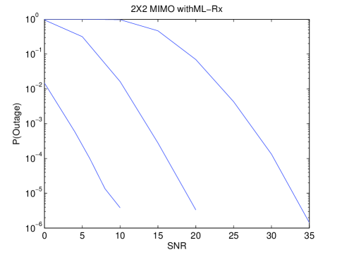
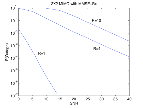
Figure 1: Outage probability of ML receiver (left) and MMSE (right) with $M=N=2$ antennas and for rates R= 1, 4, and 10 bps/Hz

In this work we seek answers for the following questions: when can the MMSE receiver exploit the full diversity in MIMO channel? More generally, how does the diversity of the MMSE receiver vary with the system parameters such as spectral efficiency $R$, the number of antennas, and in case of inter-symbol interference channel (ISI), the channel memory?

The well-known and powerful framework of diversity-multiplexing tradeoff (DMT) is not sufficient to answer the above questions, because the DMT framework cannot distinguish between different spectral efficiencies that correspond to the same multiplexing gain. In the MIMO MMSE receiver, rates that correspond to the same multiplexing gain can produce different diversities.

We approach the problem of MMSE reception in MIMO flat fading channels through a rate-dependent approximation of the outage probability and then proceed with bounding the pairwise error probability (PEP) from both sides using the outage. This leads to a closed-form expression for the diversity-rate tradeoff which reveals the relationship between diversity, spectral efficiency, and number of transmit and receive antennas. The approximation of outage and PEP as functions of rate requires more delicate handling compared with the DMT analysis, as certain ratios and terms that simply vanish in the DMT analysis are in our case relevant and must be carefully handled.

We then analyze the frequency-selective, quasi-static MIMO channel. Specifically we consider single carrier (SC) MMSE equalization under zero-padding (ZP) and cyclic-prefix (CP) transmission. SC-MMSE provides an attractive alternative to orthogonal frequency division multiplexing (OFDM) due to its low complexity and natural avoidance of the peak-to-average power ratio problem. The use of cyclic prefix and zero padding has been investigated in the literature, but the explicit tradeoff between the spectral efficiency and diversity of MIMO SC-MMSE under these two schemes has been unknown and is the subject of our work. We show that the diversity is a function of number of antennas, channel memory and spectral efficiency, and obtain the explicit tradeoff in the special case of SIMO under CP transmission.

The results of this paper fully characterize the MIMO MMSE diversity in the fixed rate flat quasi-static regime. We analyze both the cases $N\geq M$ and $N<M$, showing that in either case it is possible for the system to be limited to a diversity strictly less than $MN$. More specifically, the central result of the paper is as follows: with $M$ transmit and $N$ receive antennas (for any $N$ and $M$) the diversity is $d=\lceil\big{(}M2^{-\frac{R}{M}}-(M-N)^{+}\big{)}^{+}\rceil^{2}+|N-M|\lceil\big{(}M2^{-\frac{R}{M}}-(M-N)^{+}\big{)}^{+}\rceil$, where $(\cdot)^{+}=\max(0,\cdot)$ and $\lceil\cdot\rceil$ denotes rounding up to the next higher integer. Our results confirm and refine the earlier approximate results on the diversity of MMSE MIMO receivers that were obtained for very high and very low rates [6, 5, 7]. The MIMO MAC channel is also studied.

Some of the related literature is as follows. The performance of MMSE receiver in terms of reliability goes back to [8] where outage analysis was performed for MMSE SIMO diversity combiner in a Rayleigh fading channel with multiple interferers. In the context of point-to-point MIMO systems, Gore et al. [9] compared the performance of MMSE D-BLAST with the ordered successive cancellation V-BLAST. They show that the former has better throughput at low- and moderate SNR. Onggosanusi et al. [5] studied MMSE and zero-forcing (ZF) MIMO receivers and noticed their distinct outage performance at high-SNR, specifically for large number of transmit antennas and low spectral efficiencies $R$, but provided no analysis.

Hedayat and Nosratinia [6] considered the outage probability as a function of fixed rates $R$ under joint and separate spatial encoding, but for MMSE they obtained results only in the extremes of very high and very low rates. Kumar et al. [7] provided a DMT analysis for the system of [6] and observed that the DMT analysis does not predict the diversity of MMSE receivers at lower rates. We note that all existing analyses are limited to the case where the number of receive antennas ($N$) is greater than or equal the number of the transmit antennas ($M$).

This paper is organized as follows. Section II describes the system model. Section III finds the exponential order of outage. Section IV bounds the codeword error probabilities using the outage values, and derives the final result. Section V extends the result to the MAC channel. Section VI calculates the diversity of MIMO MMSE reception in frequency-selective block-transmission systems. Section VII provides simulations that illuminate our results.

II Linear Receivers

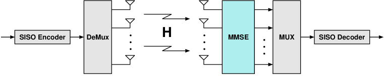
Figure 2: MIMO system with linear MMSE receiver

The input-output system model for flat fading MIMO channel with $M$ transmit and $N$ receive antennas is given by

$${\mathbf{y}}={\mathbf{H}}{\mathbf{x}}+{\mathbf{n}}$$ (1)

where ${{\mathbf{H}}\in\mathbb{C}^{N\times M}}$ is the channel matrix whose entries are independent and identically distributed complex Gaussian, ${{\mathbf{x}}\in\mathbb{C}^{\ M\times 1}}$ is the transmitted vector, ${{\mathbf{n}}\in\mathbb{C}^{\ N\times 1}}$ is the Gaussian noise vector. The vectors ${{\mathbf{x}}}$ and ${{\mathbf{n}}}$ are assumed independent. We assume a quasi-static flat fading channel and perfect channel state information (CSI) at the receiver (CSIR) and no CSI at the transmitter (CSIT), therefore transmit antennas operate with equal power.

We aim to characterize the diversity gain, $d(R,M,N)$, as a function of the spectral efficiency $R$ (bits/sec/Hz) and the number of transmit and receive antennas. This requires a pairwise error probability (PEP) analysis which is not directly tractable. Instead, we find the exponential order of outage probability and then demonstrate that outage and PEP exhibit identical exponential orders.

Following the notation of [10], we define the outage-type quantities

$$P_{out}(R,N,M) \triangleq{\mathbb{P}}(I({\mathbf{x}};{\mathbf{y}})<R)$$ (2)

$$d_{out}(R,N,M) \triangleq-\lim_{\rho\rightarrow\infty}\frac{\log P_{out}(R,M,N)}{\log\rho}$$ (3)

where $\rho$ is the per-stream signal-to-noise ratio (SNR).

We say that the two functions $f(\rho)$ and $g(\rho)$ are exponentially equal, denoted by $f(p)\doteq g(p)$ when

$$\lim_{\rho\rightarrow\infty}\frac{\log f(\rho)}{\log(\rho)}=\lim_{\rho\rightarrow\infty}\frac{\log g(\rho)}{\log(\rho)}$$

The ordering operators $\dot{\leqslant}$ and $\dot{\geqslant}$ are also defined accordingly. If $f(\rho)\doteq\rho^{d}$, we say that $d$ is the exponential order of $f(p)$.

II-A MMSE Equalizer

The equalizer, denoted by ${\mathbf{W}}$, decouples the $M$ transmitted data streams at the receiver (Figure 2). The MMSE equalizer is obtained by minimizing the mean square error (MSE) defined as ${\mathbb{E}}[||{\mathbf{x}}-{\mathbf{W}}^{H}{\mathbf{y}}||^{2}]$. It is usually assumed [6, 7] that the number of transmit antennas $M$ is no more than that of receive antennas $N$. In the following, we start with $N\geq M$ but later generalize it to $N<M$ as well.

For $N\geq M$, using the orthogonality principle, the MMSE equalizer is given by [5, 11]

$${\mathbf{W}} ={\mathbf{H}}^{H}({\mathbf{H}}{\mathbf{H}}^{H}+\rho^{-1}I)^{-1}$$

$$=({\mathbf{H}}^{H}{\mathbf{H}}+\rho^{-1}I)^{-1}{\mathbf{H}}^{H}$$ (4)

The corresponding signal-to-interference and noise ratio (SINR) of the output stream $k$ of the MMSE detector is

$$\gamma_{k} =\frac{1}{({\mathbf{I}}+\rho{\mathbf{H}}^{H}{\mathbf{H}})^{-1}_{kk}}-1,\quad 1\leqslant k\leqslant M$$ (5)

where $(\cdot)^{H}$ denotes matrix Hermitian, $(\cdot)^{-1}_{kk}$ denotes the diagonal element $k$ of the matrix inverse.

For the case $N<M$, it can be shown using a technique very similar to [8, Appendix A] that the SINR expression (5) is again valid.

The square matrix $\mathcal{W}={\mathbf{H}}^{H}{\mathbf{H}}$ is random, non-negative definite, and obeys the Wishart Distribution [12, 13]. In this work, the joint distribution of the eigenvalues of this equivalent channel matrix opens the door to the development of our analysis, as is also the case in many other MIMO results.

The equalizer output is

$${\mathbf{y}}={\mathbf{W}}{\mathbf{H}}{\mathbf{x}}+{\mathbf{W}}{\mathbf{n}}.$$ (6)

The signal streams of the transmit antennas may be either separately or jointly encoded. Separate encoding is simpler and has been fully analyzed [6], but we mention the central result for completeness.

Theorem 1 ([6, 7])

In a MIMO system consisting of $M$ transmit and $N$ receive antennas ($N\geqslant M$), under separate spatial encoding, the MMSE receiver achieves the diversity

$$d_{out}(R,N,M)=N-M+1$$ (7)

under either uniform or non-uniform rate assignment.

Furthermore, it has been established [6, 7] that the zero forcing equalizer achieves diversity $N-M+1$ under both joint or separate spatial encoding.

According to Theorem 1, a MMSE receiver operating under separate spatial encoding (e.g. horizontal encoding V-BLAST) will have no more diversity gain than ZF receiver.

III Outage Analysis

We now consider the MMSE diversity where the data stream is first encoded then multiplexed into $M$ sub-streams, each transmitted by one antenna. This approach is known to improve the performance compared with separate coding of the streams [14]. Outage occurs if the channel fails to support the target rate [12]. After channel equalization, the $M$ sub-streams $x_{k}$ are decoupled and thus the mutual information between the transmitted vector ${\mathbf{x}}$ and the received vector ${\mathbf{y}}$ given CSIR is [5]

$$I({\mathbf{x}},{\mathbf{y}})=\sum^{M}_{k=1}I(x_{k},y_{k})$$ (8)

Thus from (2) and (8), $P_{out}$ is given by

$$P_{out}={\mathbb{P}}\bigg{(}\sum^{M}_{k=1}\log(1+\gamma_{k})<R\bigg{)}$$ (9)

Substituting MMSE SINR $(\gamma_{k})$ from (5) in (9) we get

$$P_{out}={\mathbb{P}}\bigg{(}\sum^{M}_{k=1}\log({\mathbf{I}}+\rho\mathcal{W})^{-1}_{kk}>-R\bigg{)}$$ (10)

The dependence on the diagonal elements of the random matrix $({\mathbf{I}}+\rho\mathcal{W})^{-1}_{kk}$ makes further analysis intractable. We instead proceed to provide lower and upper bounds on the outage probability. In Section IV we will show that outage probability ($P_{out}$) and pairwise error probability (PEP) exhibit identical exponential error.

III-A Outage Upper Bound

Lemma 1

For an MMSE MIMO system consisting of $M$ transmit and $N$ receive antennas, under quasi-static Rayleigh fading, we have $P_{out}(R,M,N)\dot{\leqslant}\rho^{-d_{out}(R,M,N)}$ where

$$d_{out}(R,M,N) =\bigg{\lceil}\big{(}M2^{-\frac{R}{M}}-(M-N)^{+}\big{)}^{+}\bigg{\rceil}^{2}+$$

$$\hskip 10.0pt\big{|}N-M\big{|}\bigg{\lceil}\big{(}M2^{-\frac{R}{M}}-(M-N)^{+}\big{)}^{+}\bigg{\rceil}.$$ (11)

where $()^{+}$ denotes the $\max(0,\cdot)$.

Proof:

We begin by bounding the sum in (10) via Jensen’s inequality

$$\sum^{M}_{k=1}\log\big{(}{\mathbf{I}}+\rho\mathcal{W}\big{)}^{-1}_{kk} \leq M\log\big{(}\sum^{M}_{k=1}\frac{1}{M}({\mathbf{I}}+\rho\mathcal{W})^{-1}_{kk}\big{)}$$

$$=M\log\big{(}\frac{1}{M}\mathrm{tr}\big{(}({\mathbf{I}}+\rho\mathcal{W})^{-1}\big{)}\big{)}$$

$$=M\log\big{(}\frac{1}{M}\sum^{M}_{k=1}\frac{1}{1+\rho\lambda_{k}}\big{)}$$ (12)

where (12) is true because trace is equal to the sum of eigenvalues.

Notice that for $N<M$ only $N$ eigenvalues are non-zero. hence (12) can be written as

$$M\log\bigg{(}\frac{1}{M}\sum^{L}_{k=1}\frac{1}{1+\rho\lambda_{k}}+(M-N)^{+}\bigg{)}$$ (13)

where $L=\min(M,N)$.

Substituting (13) in (10), we have

$$P_{out}\leq{\mathbb{P}}\bigg{(}\sum^{L}_{k=1}\frac{1}{1+\rho\lambda_{k}}\geqslant M2^{-\frac{R}{M}}-(M-N)^{+}\bigg{)}$$ (14)

Define:

$$\alpha_{k}\triangleq-\frac{\log\lambda_{k}}{\log\rho},\quad\mathrm{for}\quad k=1,...,n\quad,$$ (15)

based on which we can write the exponential equality

$$\frac{1}{1+\rho\lambda_{k}}\doteq\begin{cases}\rho^{\alpha_{k}-1}&\mbox{$\alpha_{k}<1$ }\\ 1&\mbox{$\alpha_{k}>1$}\end{cases}$$ (16)

Define ${\boldsymbol{\alpha}}$ $=[\alpha_{1},...,\alpha_{n}]$ and a new random variable

$$M(\boldsymbol{\alpha)}\triangleq\sum_{\alpha_{k}>1}1$$ (17)

This definition is based on the observation that the term $\frac{1}{1+\rho\lambda_{k}}$ defined in (16) is either zero or one at high SNR, therefore to characterize $\sum_{k}\frac{1}{1+\rho\lambda_{k}}$ at high SNR we count the ones. Thus

$$\sum^{n}_{k=1}\frac{1}{1+\rho\lambda_{k}} \doteq\sum_{\alpha_{k}>1}1+\sum_{\alpha_{k}<1}\rho^{\alpha_{k}-1}$$ (18)

$$\doteq M({\boldsymbol{\alpha}})+\max_{\{\alpha_{k}:\alpha_{k}<1\}}{\rho^{\alpha_{k}-1}}$$ (19)

$M({\boldsymbol{\alpha}})$ inherits its randomness from $\lambda_{1},\ldots,\lambda_{n}$. The bound in (14) is evaluated by computing the probability of $\{{\boldsymbol{\alpha}}\in\mathcal{A}\}$, where $\mathcal{A}=\{\alpha:M({\boldsymbol{\alpha}})+\max_{\{\alpha_{k}:\alpha_{k}<1\}}{\rho^{\alpha_{k}-1}}>M2^{-\frac{R}{M}}-(M-N)^{+}\}$ denotes the outage event based on the approximation in (14). In order to evaluate the probability of this event we need the joint distribution of the eigenvalues, or equivalently the distribution of ${\boldsymbol{\alpha}}$. The distribution follows Wishart distribution and was initially discovered by [13] . The distribution of ${\boldsymbol{\alpha}}$ can be easily evaluated as follows [15].

Let ${\mathbf{R}}$ be an $m\times n$ ($m\geqslant n$) random matrix whose entries are $\mathcal{CN}(0,1)$. The joint PDF of the ordered random variables ${\boldsymbol{\alpha}}$ (defined in (15) for the eigenvalues of ${\mathbf{R}}^{H}{\mathbf{R}}$) is given by

$${\mathbb{P}}({\boldsymbol{\alpha}})=K^{-1}_{m,n} (\log\rho)^{n}\prod^{n}_{i=1}\rho^{-(m-n+1)\alpha_{i}}\times$$

$$\prod_{i<j}|\rho^{-\alpha_{i}}-\rho^{-\alpha_{j}}|^{2}\exp\bigg{[}-\sum_{i=1}^{n}\rho^{-\alpha_{i}}\bigg{]}$$ (20)

where $K^{-1}_{m,n}$ is a normalizing factor.

Using the distribution of ${\boldsymbol{\alpha}}$ for the defined matrix ${\mathbf{R}}$, the asymptotic outage bound is

$$P_{out}\dot{\leqslant}\int\limits_{\mathcal{A}}{\mathbb{P}}({\boldsymbol{\alpha}})d{\boldsymbol{\alpha}}$$

$$=K^{-1}_{m,n}(\log\rho)^{n}\int\limits_{\mathcal{A}}\prod^{n}_{i=1}\rho^{-(m-n+1)\alpha_{i}}\prod_{i<j}|\rho^{-\alpha_{i}}-\rho^{-\alpha_{j}}|^{2}\times$$

$$\hskip 80.0pt\exp\bigg{[}-\sum_{i=1}^{n}\rho^{-\alpha_{i}}\bigg{]}\;\text{d}{\boldsymbol{\alpha}}$$ (21)

The simplification of the integral follows from [15]. The term outside the integral has no effect on the exponent. The term $|\rho^{-\alpha_{i}}-\rho^{-\alpha_{j}}|$ is dominated by $\rho^{-\alpha_{i}}$ at high SNR. We now divide the integration range into $\mathcal{A^{\prime}}=\mathcal{A}\cap\mathbb{R}^{n}_{+}$ and its complement. If ${\boldsymbol{\alpha}}\notin\mathcal{A^{\prime}}$, the exponential term will dominate the other terms and will drive the integral to zero. If ${\boldsymbol{\alpha}}\in\mathcal{A^{\prime}}$, the exponential term is approximately 1 at high SNR and will disappear. Therefore

$$P_{out} \;\dot{\leqslant}\;\int\limits_{\mathcal{A^{\prime}}}\prod^{n}_{i=1}\rho^{-(m-n+1)\alpha_{i}}\prod_{i<j}|\rho^{-\alpha_{i}}-\rho^{-\alpha_{j}}|^{2}\;\text{d}{\boldsymbol{\alpha}}$$

$$\doteq\int\limits_{\mathcal{A^{\prime}}}\prod^{n}_{i=1}\rho^{-(2i-1+m-n)\alpha_{i}}\;\text{d}{\boldsymbol{\alpha}}$$ (22)

where

$$\mathcal{A^{\prime}} =\{M({\boldsymbol{\alpha}})>M2^{-\frac{R}{M}}-(M-N)^{+}\}$$

$$=\{\alpha_{1}>1,...,\alpha_{S}>1,\alpha_{S+1}>0,...\alpha_{L}>0\}$$ (23)

and $S=\big{\lceil}\big{(}M2^{-\frac{R}{M}}-(M-N)^{+}\big{)}^{+}\big{\rceil}$. The integration region $\mathcal{A^{\prime}}$ has boundaries that are parallel to nonnegative orthant $\mathbb{R}_{+}^{n}$, therefore the integration over multiple variables in (22) can be separated:

$$P_{out}\quad \dot{\leqslant}\quad\prod^{n}_{i=1}\int\limits_{\mathcal{A^{\prime}}}\rho^{-(2i-1+m-n)\alpha_{i}}\;\text{d}{\boldsymbol{\alpha}}$$ (24)

$$=\quad\rho^{-\sum_{i=1}^{S}(2i-1+m-n)}$$

$$=\quad\rho^{-(S^{2}+(m-n)S)},\quad\mbox{for $m\geqslant n$}$$ (25)

$$=\quad\rho^{-(S^{2}+|m-n|S)},\quad\mbox{for general $m,n$}$$ (26)

$$=\quad\rho^{-d_{out}}$$

which establishes the proof of Lemma 1.  $\Box$

III-B Outage Lower Bound

Lemma 2

For an MMSE MIMO system consisting of $M$ transmit and $N$ receive antennas (and $L=\min\{M,N\}$), operating under quasi-static Rayleigh fading, we have $P_{out}(R,M,N)\dot{\geqslant}\rho^{-d_{out}(R,M,N)}$ where

$$d_{out}(R,M,N) =\bigg{\lceil}\big{(}M2^{-\frac{R}{M}}-(M-N)^{+}\big{)}^{+}\bigg{\rceil}^{2}+$$

$$\hskip 10.0pt\big{|}N-M\big{|}\bigg{\lceil}\big{(}M2^{-\frac{R}{M}}-(M-N)^{+}\big{)}^{+}\bigg{\rceil}.$$

Proof: The lower bound is also based on Jensen’s inequality. Recall

$$P_{out} ={\mathbb{P}}\bigg{(}\sum^{M}_{k=1}\log(1+\gamma_{k})<R\bigg{)}$$

$$={\mathbb{P}}\bigg{(}\sum^{M}_{k=1}\log\frac{1}{({\mathbf{I}}+\rho\mathcal{W})^{-1}_{kk}}<R\bigg{)}$$

$$\geqslant{\mathbb{P}}\bigg{(}M\log\frac{1}{M}\sum^{M}_{k=1}\frac{1}{({\mathbf{I}}+\rho\mathcal{W})^{-1}_{kk}}<R\bigg{)}$$ (27)

Let the eigen decomposition of ${\mathbf{H}}^{H}{\mathbf{H}}$ be given by ${\mathbf{H}}^{H}{\mathbf{H}}={\mathbf{U}}^{H}\Lambda{\mathbf{U}}$ where ${\mathbf{U}}$ is unitary and $\Lambda$ is a diagonal matrix that has the eigenvalues of the Wishart matrix $\mathcal{W}$ on its diagonal. Let the vector ${\mathbf{u}}_{k}$ be the column $k$ of the matrix ${\mathbf{U}}$ and $u_{\ell k}$ be the element $\ell$ of this column, we have

$$({\mathbf{I}}+\rho\mathcal{W})^{-1}_{kk} ={\mathbf{u}}^{H}_{k}({\mathbf{I}}+\rho\Lambda)^{-1}{\mathbf{u}}_{k}$$

$$=\sum_{\ell=1}^{M}\frac{|u_{\ell k}|^{2}}{1+\rho\lambda_{\ell}}$$

$$\triangleq S_{k}.$$ (28)

Let $\bar{k}=\arg\min_{k}S_{k}$. Using (28), we can bound the sum in (27)

$$\frac{1}{M}\sum_{k=1}^{M}\frac{1}{({\mathbf{I}}+\rho\mathcal{W})^{-1}_{kk}} =\frac{1}{M}\sum_{k=1}^{M}\frac{1}{S_{k}}$$

$$\leqslant\;\frac{1}{\min_{k}S_{k}}$$ (29)

$$=\;\frac{1}{S_{\bar{k}}}$$ (30)

thus the outage bound in (27) can be further bounded using (29)

$$P_{out} \geqslant{\mathbb{P}}\bigg{(}M\log\frac{1}{M}\sum^{M}_{k=1}\frac{1}{({\mathbf{I}}+\rho\mathcal{W})^{-1}_{kk}}<R\bigg{)}$$

$$\geqslant{\mathbb{P}}\bigg{(}M\log\frac{1}{S_{\bar{k}}}<R\bigg{)}$$

$$={\mathbb{P}}\bigg{(}S_{\bar{k}}>2^{-\frac{R}{M}}\bigg{)}$$ (31)

We now bound (31) by conditioning on the event $\mathcal{B}\triangleq\big{\{}|u_{\ell\bar{k}}|^{2}\geqslant\frac{a}{M}\big{\}}$ where $a$ is a positive real number that is slightly smaller than one, i.e. $a=1-\epsilon$, and $\epsilon$ is a small positive number. We then have

$${\mathbb{P}}\bigg{(}S_{\bar{k}} >2^{-\frac{R}{M}}\bigg{)}\geqslant{\mathbb{P}}\bigg{(}S_{\bar{k}}>2^{-\frac{R}{M}}\big{|}\mathcal{B}\bigg{)}{\mathbb{P}}(\mathcal{B})$$

$$={\mathbb{P}}\bigg{(}\sum_{\ell=1}^{M}\frac{|u_{\ell\bar{k}}|^{2}}{1+\rho\lambda_{\ell}}>2^{-\frac{R}{M}}\bigg{|}\mathcal{B}\bigg{)}{\mathbb{P}}(\mathcal{B})$$

$$\geqslant{\mathbb{P}}\bigg{(}\frac{1}{M}\sum_{\ell=1}^{M}\frac{a}{1+\rho\lambda_{\ell}}>2^{-\frac{R}{M}}\bigg{)}{\mathbb{P}}(\mathcal{B})$$

$$\doteq{\mathbb{P}}\bigg{(}\frac{1}{M}\sum_{\ell=1}^{M}\frac{a}{1+\rho\lambda_{\ell}}>2^{-\frac{R}{M}}\bigg{)}$$ (32)

$$={\mathbb{P}}\bigg{(}\sum_{\ell=1}^{M}\frac{1}{1+\rho\lambda_{\ell}}>\frac{M}{a}2^{-\frac{R}{M}}\bigg{)}$$

$$={\mathbb{P}}\bigg{(}\frac{1}{M}\sum^{L}_{\ell=1}\frac{1}{1+\rho\lambda_{\ell}}>\frac{M}{a}2^{-\frac{R}{M}}-(M-N)^{+}\bigg{)}$$ (33)

where (32) follows because ${\mathbb{P}}(\mathcal{B})$ is finite and independent of $\rho$; this can be proved similarly to [7, Appendix A]. To make the upcoming expressions compact, we introduce a new variabe $\kappa\triangleq\frac{M}{a}2^{-\frac{R}{M}}-(M-N)^{+}$

$${\mathbb{P}}\bigg{(}\frac{1}{M}\sum^{L}_{\ell=1}\frac{1}{1+\rho\lambda_{\ell}}>\kappa\bigg{)}$$ (34)

Whenever $M2^{-\frac{R}{M}}$ is non-integer, the constant $a$ can be chosen such that $\big{\lceil}\big{(}M2^{-\frac{R}{M}}-(M-N)^{+}\big{)}^{+}\big{\rceil}=\big{\lceil}\big{(}\frac{M}{a}2^{-\frac{R}{M}}-(M-N)^{+}\big{)}^{+}\big{\rceil}$. We note this is satisfied for all rates, with the exception of an isolated set of points. As long as $M2^{\frac{R}{M}}\notin{\mathbb{N}}$ we have:

$$P_{out} \geqslant{\mathbb{P}}\bigg{(}\sum^{L}_{\ell=1}\frac{1}{1+\rho\lambda_{\ell}}>\kappa\bigg{)}$$

$$\doteq{\mathbb{P}}\bigg{(}\sum^{L}_{k=1}\frac{1}{1+\rho\lambda_{\ell}}>\lceil\kappa\rceil\bigg{)}$$ (35)

The remaining steps follow similarly to the proof of Lemma 1. Thus $P_{out}\;\dot{\geqslant}\;\rho^{-d_{out}}$ with $d_{out}$ is given by Lemma 2.

On the set of isolated points $M2^{-\frac{R}{M}}\in{\mathbb{N}}$, the right hand side of Eq. (35) obeys a slightly weaker upper bound by replacing $\kappa$ with $\kappa+1$. We can combine the cases where $M2^{-\frac{R}{M}}$ is integer and non-integer to write the upper bound compactly as follows:

$$d_{out}(R,M,N) \leq\bigg{\lfloor}\big{(}M2^{-\frac{R}{M}}+1-(M-N)^{+}\big{)}^{+}\bigg{\rfloor}^{2}+$$

$$\hskip 10.0pt\big{|}N-M\big{|}\bigg{\lfloor}\big{(}M2^{-\frac{R}{M}}+1-(M-N)^{+}\big{)}^{+}\bigg{\rfloor}.$$

Inspection shows that this bound is tight against the lower bound everywhere except its discontinuity points. In other words, the upper bound is left-continuous while the lower bound was right-continuous at the discontinuity points.

 $\Box$

IV PEP Analysis

Recalling that the diversity is roughly defined as the slope of PEP at high SNR, we now proceed to bound the PEP tightly from both sides using the outage results already obtained.

IV-A PEP Upper Bound

We start by a lower bound that is inspired by [15, Lemma 5] but requires a more careful treatment since we are analyzing rate, not the DMT (see the Introduction).

Lemma 3

For a quasi-static fading MIMO channel with MMSE receiver we have $d_{out}(R,M,N)\geqslant d(R,M,N)$.

Proof:

Denote $E$ for an error event, and let $x\in\mathcal{C}$ be the transmitted codeword from a codebook $\mathcal{C}$ of size $2^{Rl}$ where $R$ and $l$ are code rate and code length respectively. Define ${\boldsymbol{f}}={\mathbf{W}}{\mathbf{H}}{\mathbf{x}}$ that accounts for the combined effect of channel and equalizer. The transmit messages are assumed equi-probable so the entropy $\mathcal{H}=\log{|\mathcal{C}|}=Rl$. Applying the Fano inequality [16]

$${\mathbb{P}}(E|{\boldsymbol{f}}=f)\geqslant\frac{Rl-I({\mathbf{x}};{\mathbf{y}}|{\boldsymbol{f}}=f)}{Rl}-\frac{\mathcal{H}({\mathbb{P}}(E)|{\boldsymbol{f}}=f)}{Rl}$$ (36)

By defining $\mathcal{D}_{\delta}$ for any $\delta>0$ as $\mathcal{D}_{\delta}\triangleq\{f:I({\mathbf{x}};{\mathbf{y}}|\boldsymbol{f}=f)<l(R-\delta)\},$ and noting that $\mathcal{H}({\mathbb{P}}(E)|f\in\mathcal{D}_{\delta})\leqslant\mathcal{H}({\mathbb{P}}(E))$ from (36), we get

$${\mathbb{P}}(E|{\boldsymbol{f}}\in\mathcal{D}_{\delta}) \geqslant\frac{Rl-I({\mathbf{x}};{\mathbf{y}}|{\boldsymbol{f}}\in\mathcal{D}_{\delta})}{Rl}-\frac{\mathcal{H}({\mathbb{P}}(E))}{Rl}$$

$$\geqslant\frac{\delta}{R}-\frac{\mathcal{H}({\mathbb{P}}(E))}{Rl}.$$ (37)

Also by using the definition of $P_{out}$ we have

$${\mathbb{P}}({\boldsymbol{f}}\in\mathcal{D}_{\delta})={\mathbb{P}}\big{(}I({\mathbf{x}};{\mathbf{y}})<l(R-\delta)\big{)}\doteq\rho^{-d_{out}(R-\delta,M,N)}$$ (38)

For small enough values of $\delta>0$, we have $d_{out}(R,M,N)=d_{out}(R-\delta,M,N)$ since $d_{out}(R,M,N)$ is left-continuous with respect to $R$. Hence, by invoking (37) and (38), the error probability is given by

$${\mathbb{P}}_{\text{err}}(R,M,N) ={\mathbb{P}}(E|f\in\mathcal{D}_{\delta}){\mathbb{P}}(f\in\mathcal{D}_{\delta})+$$

$$\quad{\mathbb{P}}(E|f\notin\mathcal{D}_{\delta}){\mathbb{P}}(f\notin\mathcal{D}_{\delta})$$

$$\geqslant{\mathbb{P}}(E|f\in\mathcal{D}_{\delta}){\mathbb{P}}(f\in\mathcal{D}_{\delta})$$

$$\dot{\geqslant}\bigg{(}\frac{\delta}{R}-\frac{\mathcal{H}({\mathbb{P}}(E))}{Rl}\bigg{)}\rho^{-d_{out}}$$

$$\doteq\rho^{-d_{out}}$$ (39)

where we have used $\big{(}\frac{\delta}{R}-\frac{\mathcal{H}({\mathbb{P}}(E))}{Rl}\big{)}\doteq 1$, which was derived in [10]. This establishes the proof of the PEP upper bound.  $\Box$

IV-B PEP Lower Bound

We begin by writing the error probability in terms of error event $E$ and outage event $O$

$${\mathbb{P}}_{\text{err}}(R,M,N)={\mathbb{P}}(E|O)\cdot P_{out}+{\mathbb{P}}(E,\bar{O})\\$$

In Section III-A we have shown that, based on the event $\big{\{}\sum^{L}_{k=1}\frac{1}{1+\rho\lambda_{k}}\geqslant M2^{-\frac{R}{M}}-(M-N)^{+}\big{\}}$, the outage probability is upper bounded by $P_{out}\dot{\leqslant}\rho^{-d_{out}}$. Hence, the error probability can be bounded as

$${\mathbb{P}}_{\text{err}}(R,M,N) \dot{\leqslant}{\mathbb{P}}(E|O)\,\rho^{-d_{out}}+{\mathbb{P}}(E,\bar{O})$$

$$\leqslant\rho^{-d_{out}}+{\mathbb{P}}(E,\bar{O})$$ (40)

We intend to show that $\rho^{-d_{out}}\;\dot{\geqslant}\hskip 3.61371pt{\mathbb{P}}(E,\bar{O})$, and thus ${\mathbb{P}}_{\text{err}}(R,M,N)\;\dot{\leqslant}\;\rho^{-d_{out}}$ which produces the following lemma.

Lemma 4

For a quasi-static fading MIMO channel with MMSE receiver we have $d_{out}(R,M,N)\leqslant d(R,M,N)$.

Proof:

We begin by giving a sketch of the proof then we proceed with the details. The first part of the proof consists of developing a bound on PEP conditioned on $H$, namely $P[s_{k}\rightarrow s_{j}|{\mathbf{H}}=H]$. To do this we obtain an upper bound of the variance of the SINR which is expressed in terms of the eigenvalues of the Wishart matrix $\mathcal{W}$, resulting in ${\mathbb{P}}[E|{\mathbf{H}}=H]\leqslant 4\exp({-\big{(}\sum^{L}_{k=1}\frac{\rho\lambda_{k}}{(1+\rho\lambda_{k})^{2}}\big{)}^{-1}})\,.$ The PEP is used to derive a conditional union bound on error. We then divide the channel events into two sets based on the exponential order of the eigenvalues: the set where $M({\boldsymbol{\alpha}})=0$ and otherwise. We apply Bayes theorem on the union bound using these two sets. The calculation of the terms of the Bayesian gives ${\mathbb{P}}(E,\bar{O})\dot{\leqslant}\rho^{-MN}\leqslant\rho^{-d_{out}}$ as desired.

We now proceed in detail. We want to compute the probability that the transmitted symbol $x(k)=s_{l}$ is erroneously detected as $x(k)=s_{j}$.

Recalling the equalizer output given by (6), define the noise-plus-interference signal

$$\tilde{{\mathbf{n}}}={\mathbf{y}}-\sqrt{\rho}{\mathbf{x}}=\sqrt{\rho}({\mathbf{W}}{\mathbf{H}}-{\mathbf{I}}){\mathbf{x}}+{\mathbf{W}}{\mathbf{n}}$$ (41)

Using the eigen-decomposition of $H$ and noting that $E({\mathbf{n}})=0$ and $E({\mathbf{n}}{\mathbf{n}}^{H})=I$, we have

$$\mu_{\tilde{{\mathbf{n}}}} \triangleq E(\tilde{{\mathbf{n}}})=\sqrt{\rho}({\mathbf{W}}{\mathbf{H}}-{\mathbf{I}})=-\rho^{\frac{1}{2}}(\mathcal{W}+\rho^{-1}{\mathbf{I}})^{-1}{\mathbf{x}}$$ (42)

$$\boldsymbol{R_{\tilde{{\mathbf{n}}}}} \triangleq E(\tilde{{\mathbf{n}}}\tilde{{\mathbf{n}}}^{H})=(\mathcal{W}+\rho^{-1}{\mathbf{I}})^{-1}$$ (43)

Thus the variance of the noise sample $\tilde{n}(k)$ is given by

$$\sigma^{2}_{\tilde{{\mathbf{n}}}}(k) =\boldsymbol{R_{\tilde{{\mathbf{n}}}}}(k,k)-|\mu_{\tilde{{\mathbf{n}}}}(k)|^{2}$$

$$=(\mathcal{W}+\rho^{-1}{\mathbf{I}})^{-1}_{kk}-\rho^{-1}(\mathcal{W}+\rho^{-1}{\mathbf{I}})^{-2}_{kk}$$ (44)

where $|\mu_{\tilde{{\mathbf{n}}}}(k)|^{2}$ is the $k^{th}$ diagonal of the matrix $E(\tilde{{\mathbf{n}}})E(\tilde{{\mathbf{n}}}^{H})$ and $k$ counts from 1 to $M$.

By defining $e_{jl}\triangleq\frac{s_{j}-s_{l}}{|s_{j}-s_{l}|}$, the probability of erroneous detection for channel realization is given by

$$\begin{split}{\mathbb{P}}[s_{l}\rightarrow&s_{j}|{\mathbf{H}}=H]\\ &={\mathbb{P}}\bigg{[}\frac{\rho}{4}|s_{j}-s_{l}|^{2}\leqslant|e^{*}_{jl}(y(k)-\sqrt{\rho}s_{l})|^{2}\bigg{|}{\mathbf{H}}=H\bigg{]}\\ &\leqslant{\mathbb{P}}\bigg{[}\frac{\rho}{4}|s_{j}-s_{l}|^{2}\leqslant|\tilde{n}_{k}|^{2}\bigg{|}{\mathbf{H}}=H\bigg{]}\end{split}$$ (45)

where the inequality holds since $|e^{*}_{jl}(y(k)-\sqrt{\rho}s_{l})|\leqslant|e^{*}_{jl}||(y(k)-\sqrt{\rho}s_{l})|=|(y(k)-\sqrt{\rho}s_{j})|=|\tilde{n}(k)|$.

Denoting the real and imaginary parts of $\tilde{n}(k)$ by $\tilde{n}_{r}(k)\sim\mathcal{N}(\mu_{r}(k),\sigma^{2}_{r}(k))$ and $\tilde{n}_{i}(k)\sim\mathcal{N}(\mu_{i}(k),\sigma^{2}_{i}(k))$ respectively, we then have

$$\big{\{}\frac{\rho}{4}|s_{j}-s_{l}|^{2}\leqslant|\tilde{n}(k)|^{2}\big{\}}$$

$$\subset\big{\{}\frac{\rho}{16}|s_{j}-s_{l}|^{2}\leqslant|\tilde{n}_{r}(k)|^{2}\big{\}}\cup\big{\{}\frac{\rho}{16}|s_{j}-s_{l}|^{2}\leqslant|\tilde{n}_{i}(k)|^{2}\big{\}}$$ (46)

Applying the property of the Gaussian tail function $Q(x)\leqslant e^{(-x^{2}/2)}$ for the pairwise error probability, we obtain

$${\mathbb{P}}[s_{k}\rightarrow s_{j}|{\mathbf{H}}=H]$$

$$\leqslant e^{\bigg{(}-\frac{(\frac{\sqrt{\rho}}{4}|s_{j}-s_{l}|-\mu_{r}(k))^{2}}{\sigma_{r}^{2}(k)}\bigg{)}}+e^{\bigg{(}-\frac{(\frac{\sqrt{\rho}}{4}|s_{j}-s_{l}|+\mu_{r}(k))^{2}}{\sigma_{r}^{2}(k)}\bigg{)}}$$

$$+e^{\bigg{(}-\frac{(\frac{\sqrt{\rho}}{4}|s_{j}-s_{l}|-\mu_{i}(k))^{2}}{\sigma_{i}^{2}(k)}\bigg{)}}+e^{\bigg{(}-\frac{(\frac{\sqrt{\rho}}{4}|s_{j}-s_{l}|+\mu_{i}(k))^{2}}{\sigma_{i}^{2}(k)}\bigg{)}}$$

$$\leqslant e^{\bigg{(}-\frac{(\frac{\sqrt{\rho}}{4}|s_{j}-s_{l}|-\mu_{r}(k))^{2}}{\sigma_{\tilde{{\mathbf{n}}}}^{2}(k)}\bigg{)}}+e^{\bigg{(}-\frac{(\frac{\sqrt{\rho}}{4}|s_{j}-s_{l}|+\mu_{r}(k))^{2}}{\sigma_{\tilde{{\mathbf{n}}}}^{2}(k)}\bigg{)}}$$

$$+e^{\bigg{(}-\frac{(\frac{\sqrt{\rho}}{4}|s_{j}-s_{l}|-\mu_{i}(k))^{2}}{\sigma_{\tilde{{\mathbf{n}}}}^{2}(k)}\bigg{)}}+e^{\bigg{(}-\frac{(\frac{\sqrt{\rho}}{4}|s_{j}-s_{l}|+\mu_{i}(k))^{2}}{\sigma_{\tilde{{\mathbf{n}}}}^{2}(k)}\bigg{)}}$$ (47)

where the last step holds as $\sigma^{2}_{{\mathbf{n}}}(k)=\sigma^{2}_{r}(k)+\sigma^{2}_{i}(k)\geqslant\sigma^{2}_{r}(k),\sigma^{2}_{i}(k)$.

Now we proceed by showing that $\mu_{i}(k)\dot{\leqslant}\rho^{\frac{1}{2}}$. Consider the eigen decomposition of

$$[\mathcal{W}+\rho^{-1}{\mathbf{I}}]^{-1} =\mathbf{U}^{H}[\Lambda+\rho^{-1}{\mathbf{I}}]^{-1}\mathbf{U}$$

$$=\mathbf{U}^{H}\big{[}\text{diag}\big{\{}\frac{1}{\lambda_{k}+\rho^{-1}}\big{\}}\big{]}\mathbf{U}$$ (48)

where $\mathbf{U}$ is unitary matrix, and $\Lambda$ is the eigen decomposition of $\mathcal{W}$. Note that $\lambda_{k}+\rho^{-1}\dot{\geqslant}\rho^{-1}$ or $\frac{1}{\lambda_{k}+\rho^{-1}}\dot{\leqslant}\rho$. Therefore, all elements of the matrix $\pm\mathbf{U}^{H}[\Lambda+\rho^{-1}{\mathbf{I}}]^{-1}\mathbf{U}$, being linear combination of $\{\frac{1}{\lambda_{k}+\rho^{-1}}\}$, cannot grow faster than $O(\rho)$, and thus the elements of $\pm\rho^{\frac{1}{2}}[\mathcal{W}+\rho^{-1}{\mathbf{I}}]^{-1}$ cannot grow faster than $O(\rho^{\frac{1}{2}})$, i.e. $\pm\mu_{\tilde{{\mathbf{n}}}}(k)\dot{\leqslant{\rho^{\frac{1}{2}}}}$ and therefore $\rho^{\frac{1}{2}}\pm\mu_{\tilde{{\mathbf{n}}}}(k)\doteq\rho^{\frac{1}{2}}$. The same result holds for $\mu_{r}(k)$ and $\mu_{i}(k)$.

As a result, for any $s_{j}$ and $s_{l}$, $\frac{\sqrt{\rho}}{4}|s_{j}-s_{l}|\pm\mu_{r}(k)\doteq\rho^{\frac{1}{2}}\pm\mu_{r}(k)\doteq\rho^{\frac{1}{2}}$ and similarly $\frac{\sqrt{\rho}}{4}|s_{j}-s_{l}|\pm\mu_{i}(k)\doteq\rho^{\frac{1}{2}}$. Thus from (47), we have

$${\mathbb{P}}[s_{k}\rightarrow s_{j}|{\mathbf{H}}=H]\quad\dot{\leqslant}\quad 4e^{-\frac{\rho}{\sigma^{2}_{\tilde{{\mathbf{n}}}}(k)}}$$ (49)

Now we bound the variance in (44) and apply it in (49)

$$\sigma^{2}_{\tilde{{\mathbf{n}}}}(k) \leqslant\sum^{L}_{k=1}\bigg{[}(\mathcal{W}+\rho^{-1}{\mathbf{I}})^{-1}_{kk}-\rho^{-1}(\mathcal{W}+\rho^{-1}{\mathbf{I}})^{-2}_{kk}\bigg{]}$$

$$=\sum^{L}_{k=1}\bigg{[}\frac{\rho}{1+\rho\lambda_{k}}-\frac{\rho}{(1+\rho\lambda_{k})^{2}}\bigg{]}=\sum^{L}_{k=1}\frac{\rho^{2}\lambda_{k}}{(1+\rho\lambda_{k})^{2}}$$ (50)

Denoting the error event $E$ and using (50), the probability of erroneous detection in (49) is bounded as

$${\mathbb{P}}[E|{\mathbf{H}}=H]\leqslant 4e^{-\big{(}\sum^{L}_{k=1}\frac{\rho\lambda_{k}}{(1+\rho\lambda_{k})^{2}}\big{)}^{-1}}$$ (51)

Applying the union bound, we get

$${\mathbb{P}}(E|{\mathbf{H}}=H)\dot{\leqslant}2^{Rl}e^{-\big{(}\sum^{L}_{k=1}\frac{\rho\lambda_{k}}{(1+\rho\lambda_{k})^{2}}\big{)}^{-1}}$$ (52)

Based on (52), we can evaluate $P(E,\bar{O})$ in (40) as follows. Recalling the exponential inequality

$$\sum^{n}_{k=1}\frac{1}{1+\rho\lambda_{k}} \doteq\sum_{\alpha_{k}>1}1+\sum_{\alpha_{k}<1}\rho^{\alpha_{k}-1}$$ (53)

$$\doteq M({\boldsymbol{\alpha}})+\max_{\{\alpha_{k}:\alpha_{k}<1\}}{\rho^{\alpha_{k}-1}}$$

$$\doteq M({\boldsymbol{\alpha}})$$ (54)

Consider the two regions: $\{{\boldsymbol{\alpha}}:M({\boldsymbol{\alpha}})=0\}$ and $\{{\boldsymbol{\alpha}}:M({\boldsymbol{\alpha}})\geqslant 1\}$. At high SNR the event $\bar{O}$ is equivalent to $\{{\boldsymbol{\alpha}}:M({\boldsymbol{\alpha}})\dot{\leqslant}\lceil M2^{-\frac{R}{M}}-(M-N)^{+}\rceil\}$.

In the first region $\{M({\boldsymbol{\alpha}})=0\}$, at any rate $R\geqslant 0$ we have $\{{\boldsymbol{\alpha}}:\lceil M2^{-\frac{R}{M}}-(M-N)^{+}\rceil\dot{\geqslant}M({\boldsymbol{\alpha}})=0$ so there is no outage.

In the second region $\{M({\boldsymbol{\alpha}})\geqslant 1\}$ the exponent order of the outage probability depends on the rate. We investigate these two regions separately.

In the region $\{{\boldsymbol{\alpha}}:M({\boldsymbol{\alpha}})=0\}$, we have $\max_{k}\alpha_{k}<1$ since all $\alpha_{k}^{\prime}s<1$. From (52) and (54) we conclude that

$${\mathbb{P}}(E,\bar{O}|M({\boldsymbol{\alpha}})=0) \dot{\leqslant}2^{Rl}e^{-\rho^{\big{(}\max_{k}\alpha_{k}-1\big{)}^{-1}}}$$

$$=2^{Rl}e^{-\rho^{\big{(}1-\max_{k}\alpha_{k}\big{)}}}$$ (55)

Since exponential function dominates all polynomials and $1-\max_{k}\alpha_{k}>0$, we get

$$\lim_{\rho\rightarrow\infty}\frac{e^{-\rho^{\big{(}1-\max_{k}\alpha_{k}\big{)}}}}{\rho^{-MN}}=0$$

which in turn yields

$${\mathbb{P}}(E,\bar{O}|M({\boldsymbol{\alpha}})=0) \dot{\leqslant}2^{Rl}e^{-\rho^{\big{(}1-\max_{k}\alpha_{k}\big{)}}}$$

$$\dot{\leqslant}\rho^{-MN}$$ (56)

We next show that the same result holds for the other region $\{{\boldsymbol{\alpha}}:M({\boldsymbol{\alpha}})\geqslant 1\}$.

Following the same line of argument as we did for (56) but for $M({\boldsymbol{\alpha}})\geqslant 1$, we have

$$P(E,\bar{O}|M({\boldsymbol{\alpha}})\geqslant 1) \;\dot{\leqslant}\;2^{Rl}e^{-\big{(}\sum^{L}_{k=1}\frac{\rho\lambda_{k}}{(1+\rho\lambda_{k})^{2}}\big{)}^{-1}}$$

$$\leqslant e^{2^{Rl}}e^{-\big{(}\sum_{k}\frac{1}{1+\rho\lambda}-\sum_{k}\frac{\rho\lambda_{k}}{(1:\rho\lambda_{k})^{2}}\big{)}^{-1}}$$

$$=e^{2^{Rl}}\underbrace{e^{-\big{(}\sum_{k}\frac{1}{1+\rho\lambda_{k}}\big{)}^{-1}}}_{\dot{\leqslant}1\text{ since }M({\boldsymbol{\alpha}})\geqslant 1}\times$$

$$\qquad e^{\bigg{[}-\frac{\sum_{k}\frac{1}{(\rho\lambda_{k}+1)^{2}}}{\big{(}\sum_{k}\frac{1}{1+\rho\lambda_{k}}\big{)}\big{(}\sum_{k}\frac{\rho\lambda_{k}}{(1+\rho\lambda_{k})^{2}}\big{)}}\bigg{]}}$$

$$\;\dot{\leqslant}\;e^{2^{Rl}}e^{\big{[}-\frac{LM({\boldsymbol{\alpha}})}{LM({\boldsymbol{\alpha}})\rho^{-\min_{k}|1-\alpha_{k}|}}\big{]}}$$ (57)

$$\doteq e^{-\rho^{\min_{k}|1-\alpha_{k}|}}$$

$$\;\dot{\leqslant}\;e^{\rho^{1-\max_{k}\alpha_{k}}}\;\dot{\leqslant}\;\rho^{-MN}$$ (58)

where (57) is direct application of (54) for $M({\boldsymbol{\alpha}})\geqslant 1$, and (58) follows from the fact that $|1-\alpha_{k}|\geqslant 1$. Note that (58) is true for any code length $l$. Invoking the results of (56) and (58), we can now evaluate ${\mathbb{P}}(E,\bar{\mathcal{C}})$ as follows

$${\mathbb{P}}(E,\bar{O}) =\int\limits_{M({\boldsymbol{\alpha}})=0}{\mathbb{P}}(E,\bar{O}|M({\boldsymbol{\alpha}})=0){\mathbb{P}}({\boldsymbol{\alpha}})\text{d}{\boldsymbol{\alpha}}$$

$$+\int\limits_{M({\boldsymbol{\alpha}})\geqslant 1}{\mathbb{P}}(E,\bar{O}|M({\boldsymbol{\alpha}})\geqslant 1){\mathbb{P}}({\boldsymbol{\alpha}})\text{d}{\boldsymbol{\alpha}}$$ (59)

$$\;\dot{\leqslant}\;\rho^{-MN}\int\limits_{M({\boldsymbol{\alpha}})=0}{\mathbb{P}}({\boldsymbol{\alpha}})\text{d}{\boldsymbol{\alpha}}+\rho^{-MN}\int\limits_{M({\boldsymbol{\alpha}})\geqslant 1}{\mathbb{P}}({\boldsymbol{\alpha}})\text{d}{\boldsymbol{\alpha}}$$ (60)

$$\doteq\rho^{-MN}$$ (61)

Therefore, ${\mathbb{P}}(E,\bar{O})\dot{\leqslant}\rho^{-MN}$ for all regions of ${\boldsymbol{\alpha}}$. Finally, (40) becomes

$${\mathbb{P}}_{\text{err}}(R,M,N) \;\dot{\leqslant}\;{\mathbb{P}}(E|O)\;\rho^{-d_{out}}+{\mathbb{P}}(E,\bar{O})$$

$$\leqslant\rho^{-d_{out}}+{\mathbb{P}}(E,\bar{O})$$

$$\doteq\rho^{-d_{out}}+\rho^{-MN}$$

$$\doteq\rho^{-d_{out}}$$

$$=P_{out}(R,M,N)$$ (62)

which establishes the lemma.  $\Box$

From Lemma 3 and Lemma 4, we thus get

Theorem 2

For MMSE MIMO Receiver under quasi-static channel and joint spatial encoding, the pairwise error probability (PEP) and the outage probability $P_{out}$ are exponentially equal and the diversity gain is $d(R,M,N)=d_{out}(R,M,N)$, where $d_{out}(R,M,N)$ is given in (11).

V Multiple-Access Channel (MAC)

We now extend the result to the MAC channel. Consider a MIMO MAC channel with $K$ users, $M$ transmit antennas per user, $N$ receive antennas (there is no condition on $M,N$ and $k$). Assume flat fading MIMO channel, the system model is given by

$${\mathbf{y}}=\sum_{i=1}^{K}{\mathbf{H}}_{i}{\mathbf{x}}_{i}+{\mathbf{n}}={\mathbf{H_{e}}}{\mathbf{X}}+{\mathbf{n}}$$ (63)

where ${{\mathbf{H}}_{i}\in\mathbb{C}^{N\times M}}$ is the user $i$ channel matrix whose entries are independent and identically distributed complex Gaussian, ${\mathbf{H_{e}}}=[{\mathbf{H}}_{1}{\mathbf{H}}_{2}\dots\mathbf{H}_{K}]$ is the overall equivalent channel matrix, ${{\mathbf{x}}_{i}\in\mathbb{C}^{\ M\times 1}}$ is the transmitted vector of user $i$, ${\mathbf{X}}=[{\mathbf{x}}_{1}^{T}{\mathbf{x}}_{2}^{T}\dots\mathbf{x}_{K}^{T}]^{T}$ is the overall transmitted vector, and ${{\mathbf{n}}\in\mathbb{C}^{\ N\times 1}}$ is the Gaussian noise vector. The vectors ${{\mathbf{X}}}$ and ${{\mathbf{n}}}$ are assumed independent. We keep the same assumptions about the channel. That is we assume a quasi-static flat fading channel and perfect CSIR and no CSIT. We have the following theorem

Theorem 3

In a MIMO MAC system with MMSE receiver consisting of $K$ users, $M$ transmit antennas per user and $N$ receive antennas, the lower and upper bounds on the per user diversity are respectively given by $d^{\text{MAC}}_{L}(R)$ and $d^{\text{MAC}}_{U}(R)$,

$$d^{\text{MAC}}_{L}(R) =\bigg{\lceil}\big{(}M2^{-R/M}-(M-N)^{+}\big{)}^{+}\bigg{\rceil}^{2}+$$

$$\hskip 20.0pt\big{|}N-KM\big{|}\bigg{\lceil}\big{(}M2^{-R/M}-(M-N)^{+}\big{)}^{+}\bigg{\rceil}$$ (64)

$$d^{\text{MAC}}_{U}(R) =\bigg{\lceil}\big{(}KM2^{-R/{KM}}-(M-N)^{+}\big{)}^{+}\bigg{\rceil}^{2}+$$

$$\hskip 20.0pt\big{|}N-KM\big{|}\bigg{\lceil}\big{(}KM2^{-R/{KM}}-(M-N)^{+}\big{)}^{+}\bigg{\rceil}.$$ (65)

From (64) it is straightforward to verify the single user case. The machinery of the proof is mostly similar to the single user case. However, the outage upper and lower bounds are obtained in a different manner that is pointed out in the following analysis for $N\geqslant M$. The case $N<M$ can be similarly obtained.

V-A MAC Outage Upper Bound

The user $i$ outage probability can be written as

$$P^{i}_{out}={\mathbb{P}}\bigg{(}\sum^{iM}_{k=(i-1)M+1}\log(1+\gamma^{i}_{k})<R\bigg{)}.$$ (66)

where $\gamma^{i}_{k}$ is the SINR of the stream $k$ of user $i$. Specializing this to MMSE receiver we get

$$P^{i}_{out}={\mathbb{P}}\bigg{(}\sum^{iM}_{k=(i-1)M+1}\log({\mathbf{I}}+\rho{\mathbf{H_{e}}}^{H}{\mathbf{H_{e}}})^{-1}_{kk}>-R\bigg{)}.$$ (67)

Using Jensen’s Inequality the outage probability can be bounded as

$$P^{i}_{out} \leqslant{\mathbb{P}}\big{(}\log\big{(}\!\!\!\!\!\!\!\sum^{iM}_{k=(i-1)M+1}\!\!\frac{1}{M}({\mathbf{I}}+\rho{\mathbf{H_{e}}}^{H}{\mathbf{H_{e}}})^{-1}_{kk}\big{)}>\frac{-R}{M}\big{)}$$

$$\leqslant{\mathbb{P}}\big{(}\log\big{(}\sum^{KM}_{k=1}\frac{1}{M}({\mathbf{I}}+\rho{\mathbf{H_{e}}}^{H}{\mathbf{H_{e}}})^{-1}_{kk}\big{)}>\frac{-R}{M}\big{)}$$ (68)

$$={\mathbb{P}}\big{(}\sum^{KM}_{k=1}\frac{1}{1+\rho\lambda_{k}}>M2^{-\frac{R}{M}}\big{)}$$ (69)

where (68) is true since the summation in the left-hand side of the inequality adds more positive terms (recall that $({\mathbf{I}}+\rho{\mathbf{H_{e}}}^{H}{\mathbf{H_{e}}})$ is a positive definite matrix [12]). Following similar steps that were used to obtain (26) we can easily show that $P^{i}_{out}\;\dot{\leqslant}\;\rho^{-d^{\text{MAC}}_{L}}$, where $d^{\text{MAC}}_{L}$ is given by (64).

V-B MAC Outage Lower Bound

The outage probability can be lower bounded as follows

$$P^{i}_{out} ={\mathbb{P}}\bigg{(}\sum^{iM}_{k=(i-1)M+1}\log({\mathbf{I}}+\rho{\mathbf{H_{e}}}^{H}{\mathbf{H_{e}}})^{-1}_{kk}>-R\bigg{)}$$

$$\geqslant{\mathbb{P}}\bigg{(}\sum^{KM}_{k=1}\log({\mathbf{I}}+\rho{\mathbf{H_{e}}}^{H}{\mathbf{H_{e}}})^{-1}_{kk}>-R\bigg{)}$$ (70)

$$\;\dot{\geqslant}\;{\mathbb{P}}\bigg{(}\sum^{KM}_{k=1}({\mathbf{I}}+\rho{\mathbf{H_{e}}}^{H}{\mathbf{H_{e}}})^{-1}_{kk}>\frac{KM}{a}2^{\frac{-R}{M}}\bigg{)}$$ (71)

where (70) is a trivial bound based on dedicating all $KM$ antennas to one user, and (71) uses the same technique as in Section III-B, and $a$ is a positive number slightly less than one. Following similar steps that were used to obtain (26) we can easily show that $P^{i}_{out}\;\dot{\geqslant}\;\rho^{-d^{\text{MAC}}_{U}}$, where $d^{\text{MAC}}_{U}$ is given by (65).

VI Frequency-Selective Channel

Broadband wireless systems usually operate in frequency-selective channels where, in addition to the spatial diversity obtained in MIMO broadband systems, frequency diversity can be achieved. Broadband systems usually employ orthogonal frequency division multiplexing (OFDM) or single carrier (SC) transmission [17]. Specifically, SC was shown to be attractive for broadband wireless channels due to its lower complexity, lower peak-to-average power ratio and reduced sensitivity to carrier frequency errors compared to OFDM [18, 17].

In this section, we investigate the diversity achieved by SC-MMSE receivers for two block transmission schemes, namely cyclic prefix (CP) and zero-padding (ZP) schemes. The CP and ZP are commonly used for guard intervals in block quasi-static channels. Although CP was initially proposed for both single carrier and multi-carrier systems, ZP was lately shown to be an attractive alternative for both systems [19, 20].

VI-A System Model

We consider a general MIMO system in a rich scattering quasi-static environment. The equivalent baseband channel is given by multipath model with $\nu$ paths referred to as the ISI channel in the sequel. The $(\nu+1)$-tap channel impulse response between the transmit antenna $m$ and receive antenna $n$ is denoted by the vector ${\mathbf{h}}_{mn}=[h_{mn,0},h_{mn,1},\dots,h_{mn,\nu}]$. We assume a block-fading model where ${\mathbf{h}}_{mn}$ remains unchanged during a transmission block. Assuming $M$ transmit and $N$ receive antennas, the received vector ${\mathbf{y}}_{k}$ at time instant $k$ is given by [21, 10]

$${\mathbf{y}}_{k}=\sum^{\nu}_{i=0}{\mathbf{H}}_{i}{\mathbf{x}}_{k-i}+{\mathbf{n}}_{k}$$ (72)

where ${\mathbf{H}}_{i}$ is the $M\times N$ channel matrix that has $h_{mn,i}$ as its $(m,n)$ element, ${\mathbf{x}}_{k-i}$ is $M\times 1$ transmitted vector at time index $k-i$, ${\mathbf{y}}_{k}$ is the $N\times 1$ received vector and ${\mathbf{n}}_{k}$ is the $N\times 1$ Gaussian noise vector at time index $k$.

Consider a transmission of $L_{d}+L_{e}$ spatial vectors each of size $M\times 1$, where $L_{d}$ is an integer representing the number of transmissions over the quasi-static channel and $L_{e}$ is the length of data extension to avoid inter-block interference, in the form of either zero-padding or cyclic prefix. The receiver discards the $L_{e}$ vectors in the case of cyclic-prefix transmission [21]. Stacking the transmitted vector in an $M(L_{d}+L_{e})\times 1$ vector, we can write the stacked $M(L_{d}+L_{e})\times 1$ transmitted as follows

$$\bar{{\mathbf{x}}}_{k} =[{\mathbf{x}}^{T}_{k(L_{d}+L_{e})},\dots,{\mathbf{x}}^{T}_{k(L_{d}+L_{e})+L_{d}+L_{e}-1}]$$

We can then rewrite (72) as

$$\bar{{\mathbf{y}}}_{cp}=\bar{{\mathbf{H}}}\,\bar{{\mathbf{x}}}+\bar{{\mathbf{n}}}$$ (73)

where $\bar{{\mathbf{y}}}_{cp}$ is the $NL_{d}\times 1$ received vector, $\bar{{\mathbf{x}}}$ is the $M(L_{d}+L_{e})\times 1$ transmitted vector, $\bar{{\mathbf{n}}}$ is the white Gaussian noise vector $\in\mathbb{C}^{\ NL_{d}\times 1}$ and $\bar{{\mathbf{H}}}$ is the channel matrix given by

$$\bar{{\mathbf{H}}}=\begin{bmatrix}{\mathbf{H}}_{0}&{\mathbf{H}}_{1}&\cdots&{\mathbf{H}}_{\nu}&0&\cdots&0\\ 0&{\mathbf{H}}_{0}&{\mathbf{H}}_{1}&\cdots&{\mathbf{H}}_{\nu}&\cdots&0\\ \vdots&\ddots&\ddots&\ddots&\ddots&\vdots\\ 0&\cdots&\cdots&{\mathbf{H}}_{0}&{\mathbf{H}}_{1}&\cdots&{\mathbf{H}}_{\nu}\end{bmatrix}.$$ (74)

The linear data extension operation maps the data vector $\hat{{\mathbf{x}}}$ to the transmitted vector $\bar{{\mathbf{x}}}$ and is shown by

$$\bar{\mathbf{x}}=\mathbf{U_{cp}}\hat{{\mathbf{x}}}$$ (75)

where $\mathbf{U_{cp}}$ is given by

$$\mathbf{U_{cp}}=\left[\begin{array}[]{ c c }{\mathbf{I}}_{ML_{d}}\\ {\mathbf{I}}_{ML_{e}}\quad\quad{\boldsymbol{0}}_{ML_{e}\times(L_{d}-L_{e})M}\end{array}\right]$$ (76)

The system model in (73) can now be written in terms of the unpadded data vector $\hat{{\mathbf{x}}}$ and an equivalent channel matrix ${\mathbf{H_{e}}}$ as follows

$$\bar{\mathbf{y}}_{cp}={{\mathbf{H_{e}}}}\,\hat{{\mathbf{x}}}+\bar{\mathbf{n}}$$ (77)

where in a CP system, ${\mathbf{H_{e}}}=\bar{\mathbf{H}}\mathbf{U_{cp}}$ is a $NL_{d}\times ML_{d}$ block circulant matrix constructed by block circulations of the matrix $[{\mathbf{H}}_{0},{\mathbf{H}}_{1},\dots,{\mathbf{H}}_{\nu},0,\dots,0]^{T}$.

For the zero-padding transmission, we can rewrite (72) as

$$\bar{{\mathbf{y}}}_{zp}={\mathbf{H_{e}}}\,\hat{{\mathbf{x}}}+\bar{{\mathbf{n}}}$$ (78)

where $\bar{{\mathbf{y}}}_{zp}$ is the $N(L_{d}+L_{e})\times 1$ received vector, $\bar{{\mathbf{x}}}$ is the $ML_{d}\times 1$ transmitted vector, $\bar{{\mathbf{n}}}$ is the white Gaussian noise vector $\in\mathbb{C}^{N(L_{d}+L_{e})\times 1}$ and $\bar{{\mathbf{H}}}$ is the channel matrix given by

$${\mathbf{H_{e}}}=\begin{bmatrix}{\mathbf{H}}_{0}&0&\cdots&0\\ \vdots&{\mathbf{H}}_{1}&\ddots&\vdots\\ {\mathbf{H}}_{\nu}&\vdots&\ddots&{\mathbf{H}}_{0}\\ 0&{\mathbf{H}}_{\nu}&\ddots&\vdots\\ \vdots&\vdots&\vdots&{\mathbf{H}}_{\nu}\end{bmatrix}.$$ (79)

Assuming perfect channel state information at the receiver (CSIR) and that the channel remains unchanged during the transmission of $L_{d}+L_{e}$ vectors, the MMSE equalizer ${\mathbf{W}}$ is applied to decouple the received streams (after removing the $L_{e}$ extension vectors in case of cyclic-prefix transmission). The MMSE equalizer is given by

$${\mathbf{W}}=(\rho^{-1}{\mathbf{I}}+{\mathbf{H_{e}}}^{H}{\mathbf{H_{e}}})^{-1}{\mathbf{H_{e}}}^{H}$$ (80)

and the unbiased decision-point SINRs of the equalizers output for detecting the $k^{th}$ transmitted stream are

$$\gamma_{k}=\frac{1}{({\mathbf{I}}+\rho{\mathbf{H_{e}}}^{H}{\mathbf{H_{e}}})^{-1}_{kk}}-1\quad\quad k=1,\dots,ML_{d}.$$ (81)

In the following sections we analyze the outage diversity for the ZP and CP systems. The PEP analysis follows in a direct manner as in the flat fading case so we omit it.

VI-B The Zero Padding MMSE Receiver

It is known that in a point-to-point single-antenna ISI channel, linear receivers can achieve full multipath diversity under zero-padding transmission [22, 23, 20]. In this section we investigate the similar question for MIMO systems whose receivers use linear MMSE operations in both the spatial and temporal dimensions. We provide lower and upper bounds on diversity. The bounds are not always tight, but the diversity is fully characterized for SIMO systems.

We begin by analyzing the tradeoff between the spectral efficiency $R$ and the diversity of MMSE receiver in the single-antenna ISI channel $d^{ISI}_{MMSE}$ under ZP transmission. Tajer et al [10] shows that $d^{ISI}_{MMSE}$ varies with $R$ under CP transmission and MMSE equalization, in particular, for a quasi-static single-antenna ISI channel with $\nu+1$ taps, the diversity of the SC-MMSE receiver under CP transmission is $d^{CP}_{MMSE}=1+\min(\nu,\lfloor 2^{-R}L_{d}\rfloor)$, where $L_{d}$ is the transmission data block length. We show that the same is not true for ZP transmission.

Lemma 5

For a quasi-static single-antenna ISI channel with $\nu+1$ taps, the diversity of the SC-MMSE receiver under ZP transmission is $d^{ZP}_{MMSE}=\nu+1$ irrespective of $R$.

Proof:

See Appendix -A. ∎

We proceed with lower and upper bounds on diversity for MIMO ISI channel.

VI-B1 Diversity Upper Bound

Applying the MMSE equalizer given by (80) to the received vector in (77), the effective mutual information between $\hat{{\mathbf{x}}}$ and ${\mathbf{W}}\bar{{\mathbf{y}}}$ is equal to the sum of mutual information of their components [5]

$$I(\hat{{\mathbf{x}}},{\mathbf{W}}\bar{{\mathbf{y}}})=\frac{1}{L_{d}}\sum^{ML_{d}}_{k=1}I(x_{k},y_{k}).$$

Thus the outage probability is given by

$$P_{out} ={\mathbb{P}}\bigg{(}\frac{1}{L_{d}}\sum^{ML_{d}}_{k=1}\log(1+\gamma_{k})<R\bigg{)}$$ (82)

$$={\mathbb{P}}\bigg{(}\frac{1}{L_{d}}\sum^{ML_{d}}_{k=1}\log\frac{1}{({\mathbf{I}}+\rho{\mathbf{H_{e}}}^{H}{\mathbf{H_{e}}})^{-1}_{kk}}<R\bigg{)}$$ (83)

$$\geqslant{\mathbb{P}}\bigg{(}M\log\frac{1}{ML_{d}}\sum^{ML_{d}}_{k=1}\frac{1}{({\mathbf{I}}+\rho{\mathbf{H_{e}}}^{H}{\mathbf{H_{e}}})^{-1}_{kk}}<R\bigg{)}$$ (84)

where we have used Jensen’s inequality as in Section III-B. Let the eigen decomposition of ${\mathbf{H_{e}}}^{H}{\mathbf{H_{e}}}$ be given by ${\mathbf{H_{e}}}^{H}{\mathbf{H_{e}}}={\mathbf{U}}^{H}\Lambda{\mathbf{U}}$ where ${\mathbf{U}}$ is unitary and $\Lambda$ is a diagonal matrix that has the eigenvalues of the matrix ${\mathbf{H_{e}}}^{H}{\mathbf{H_{e}}}$ on its diagonal. Let the eigenvalues of ${\mathbf{H_{e}}}^{H}{\mathbf{H_{e}}}$ be given by $\{\lambda_{\ell}\}$ with $\lambda_{1}\geqslant\lambda_{2}\cdots\geqslant\lambda_{ML_{d}}$. Let the vector ${\mathbf{u}}_{k}$ be the column $k$ of the matrix ${\mathbf{U}}$, we have

$$({\mathbf{I}}+\rho{\mathbf{H_{e}}}^{H}{\mathbf{H_{e}}})^{-1}_{kk} ={\mathbf{u}}^{H}_{k}({\mathbf{I}}+\rho\Lambda)^{-1}{\mathbf{u}}_{k}$$

$$=\sum_{\ell=1}^{ML_{d}}\frac{|u_{\ell k}|^{2}}{1+\rho\lambda_{\ell}}$$

$$\triangleq S_{k}.$$

Let $\bar{k}=\arg\min_{k}S_{k}$. we can bound the sum in (84)

$$\frac{1}{ML_{d}}\sum_{k=1}^{ML_{d}}\frac{1}{({\mathbf{I}}+\rho{\mathbf{H_{e}}}^{H}{\mathbf{H_{e}}})^{-1}_{kk}} =\frac{1}{ML_{d}}\sum_{k=1}^{ML_{d}}\frac{1}{S_{k}}$$

$$\leqslant\;\frac{1}{\min_{k}S_{k}}$$

$$=\;\frac{1}{S_{\bar{k}}}$$ (85)

thus the outage bound in (84) can be further bounded

$$P_{out} \geqslant{\mathbb{P}}\bigg{(}M\log\frac{1}{ML_{d}}\sum^{M}_{k=1}\frac{1}{({\mathbf{I}}+\rho{\mathbf{H_{e}}}^{H}{\mathbf{H_{e}}})^{-1}_{kk}}<R\bigg{)}$$

$$\geqslant{\mathbb{P}}\bigg{(}M\log\frac{1}{S_{\bar{k}}}<R\bigg{)}$$

$$={\mathbb{P}}\bigg{(}S_{\bar{k}}>2^{-\frac{R}{M}}\bigg{)}$$ (86)

We now bound (86) by conditioning on the event

$$\mathcal{B}\triangleq \bigg{\{}|u_{\ell\bar{k}}|^{2}\geqslant\frac{a}{M},\;\ell=ML_{d}-M+1,\cdots,ML_{d}\bigg{\}}$$ (87)

where $a$ is a positive real number that is slightly smaller than one $a=1-\epsilon_{1}$, and $\epsilon_{1}$ is a small positive number. We then have

$$P_{out} ={\mathbb{P}}\bigg{(}S_{\bar{k}}>2^{-\frac{R}{M}}\bigg{)}$$

$$\geqslant{\mathbb{P}}\bigg{(}S_{\bar{k}}>2^{-\frac{R}{M}}\big{|}\mathcal{B}\bigg{)}{\mathbb{P}}(\mathcal{B})$$

$$={\mathbb{P}}\bigg{(}\sum_{\ell=1}^{ML_{d}}\frac{|u_{\ell\bar{k}}|^{2}}{1+\rho\lambda_{\ell}}>2^{-\frac{R}{M}}\bigg{|}\mathcal{B}\bigg{)}{\mathbb{P}}(\mathcal{B})$$

$$\geqslant{\mathbb{P}}\bigg{(}\sum_{\ell=ML_{d}-M+1}^{ML_{d}}\frac{|u_{\ell\bar{k}}|^{2}}{1+\rho\lambda_{\ell}}>2^{-\frac{R}{M}}\bigg{|}\mathcal{B}\bigg{)}{\mathbb{P}}(\mathcal{B})$$ (88)

$$\geqslant{\mathbb{P}}\bigg{(}\frac{1}{M}\sum_{\ell=ML_{d}-M+1}^{ML_{d}}\frac{a}{1+\rho\lambda_{\ell}}>2^{-\frac{R}{M}}\bigg{)}{\mathbb{P}}(\mathcal{B})$$

$$\doteq{\mathbb{P}}\bigg{(}\frac{1}{M}\sum_{\ell=ML_{d}-M+1}^{ML_{d}}\frac{a}{1+\rho\lambda_{\ell}}>2^{-\frac{R}{M}}\bigg{)}$$ (89)

$$={\mathbb{P}}\bigg{(}\sum_{\ell=ML_{d}-M+1}^{ML_{d}}\frac{1}{1+\rho\lambda_{\ell}}>\frac{M}{a}2^{-\frac{R}{M}}\bigg{)}$$ (90)

where (88) follows by removing some of the elements of the sum corresponding to the largest eigenvalues. The steps used to obtain Eq. (89) are similar to the steps used in Section III-B.

Note that ${\mathbf{H_{e}}}^{H}{\mathbf{H_{e}}}$ is not a Wishart matrix, hence the analysis of Section II does not directly apply here. The block diagonal elements of ${\mathbf{H_{e}}}^{H}{\mathbf{H_{e}}}$ are similar and are given by

$$\mathbf{D}=\sum^{\nu}_{i=0}{\mathbf{H}}_{i}^{H}{\mathbf{H}}_{i}.$$ (91)

The matrix ${\mathbf{H_{e}}}^{H}{\mathbf{H_{e}}}$ is Toeplitz and Hermitian. Moreover, the matrix $\mathbf{D}$ given by (91) is a Wishart matrix.

Observe that the probability in (90) depends on the $M$ smallest eigenvalues. We now bound these eigenvalues with the eigenvalues of the matrix ${\mathbf{D}}$ via the Sturmian separation theorem [24, P.1077].

Theorem 4

(Sturmian Separation Theorem) Let $\{\mathbf{A}_{r},r=1,2,\ldots\}$ be a sequence of symmetric $r\times r$ matrices such that each $\mathbf{A}_{r}$ is a submatrix of $\mathbf{A}_{r+1}$. Then if $\{\lambda_{k}{(\mathbf{A}_{r})}\;,\;k=1,\ldots,r\}$ denote the ordered eigenvalues of each matrix $\mathbf{A}_{r}$ in descending order, we have

$$\lambda_{k+1}(\mathbf{A}_{i+1})\leq\lambda_{k}(\mathbf{A}_{i})\leq\lambda_{k}(\mathbf{A}_{i+1}).$$

For our purposes, we consider a special case of the Sturmian Theorem by constructing a set of matrices $\mathbf{A}_{M},\mathbf{A}_{M+1},\ldots,\mathbf{A}_{L_{d}M}$ starting by the largest one $\mathbf{A}_{L_{d}M}\stackrel{{\scriptstyle\triangle}}{{=}}{\mathbf{H_{e}}}^{H}{\mathbf{H_{e}}}$ and making all other matrices $\mathbf{A}_{i}$ to be (successively embedded) $i\times i$ principal submatrices of ${\mathbf{H_{e}}}^{H}{\mathbf{H_{e}}}$, such that the smallest matrix is $\mathbf{A}_{M}=\mathbf{D}_{L_{d}}$. Then we repeatedly apply the first inequality in the Sturmian to get:

$$\lambda_{ML_{d}}(\mathbf{A}_{ML_{d}}) \leq\lambda_{ML_{d}-1}(\mathbf{A}_{ML_{d}-1}) \leq\cdots \leq\lambda_{M}(\mathbf{A}_{M})$$

$$\lambda_{ML_{d}-1}(\mathbf{A}_{ML_{d}}) \leq\lambda_{ML_{d}-2}(\mathbf{A}_{ML_{d}-1}) \leq\cdots \leq\lambda_{M-1}(\mathbf{A}_{M})$$

$$\vdots \vdots$$

$$\lambda_{ML_{d}-M+1}(\mathbf{A}_{ML_{d}}) \leq\lambda_{ML_{d}-M}(\mathbf{A}_{ML_{d}-1}) \leq\cdots \leq\lambda_{1}(\mathbf{A}_{M})$$

This implies that the smallest $M$ eigenvalues of ${\mathbf{H_{e}}}^{H}{\mathbf{H_{e}}}$ are bounded above by the $M$ eigenvalues of $\mathbf{D}$, respectively. Hence:

$$P_{out}\dot{\geqslant}\hskip 4.0pt{\mathbb{P}}\big{(}\sum^{M}_{k=1}\frac{1}{1+\rho\lambda_{k}(\mathbf{D})}>\frac{M}{a}2^{-\frac{R}{M}}\big{)}.$$ (92)

$\mathbf{D}$ is a sum of $(\nu+1)$ central Wishart matrices each with $N$ degrees of freedom and with identity covariance matrix, i.e. $\mathbf{D}\in\mathcal{W}((\nu+1)N,I)$. Therefore the analysis of Section II applies here and we have the following lemma.

Lemma 6

In a MIMO quasi-static frequency-selective system (with channel memory $\nu$) consisting of $M$ transmit and $N$ receive antennas, the MMSE receiver diversity under joint spatial encoding and zero-padding transmission is upper bounded as

$$d^{ZP}\leqslant \bigg{\lfloor}\big{(}M2^{-\frac{R}{M}}+1-(M-N)^{+}\big{)}^{+}\bigg{\rfloor}^{2}$$

$$+\big{|}(\nu+1)N-M\big{|}\bigg{\lfloor}\big{(}M2^{-\frac{R}{M}}+1-(M-N)^{+}\big{)}^{+}\bigg{\rfloor}$$ (93)

VI-B2 Diversity Lower Bound

We can upper bound the outage probability as follows.

$$P_{out}={\mathbb{P}}\bigg{(}\frac{1}{L_{d}}\sum^{ML_{d}}_{k=1}\log(1+\gamma_{k})<R\bigg{)}$$

$$={\mathbb{P}}\bigg{(}\frac{1}{L_{d}}\sum^{ML_{d}}_{k=1}\log({\mathbf{I}}+\rho{\mathbf{H_{e}}}^{H}{\mathbf{H_{e}}})^{-1}_{kk}>-R\bigg{)}$$

$$\leqslant{\mathbb{P}}\bigg{(}M\log\frac{1}{ML_{d}}\sum^{ML_{d}}_{k=1}({\mathbf{I}}+\rho{\mathbf{H_{e}}}^{H}{\mathbf{H_{e}}})^{-1}_{kk}>-R\bigg{)}$$ (94)

$$\leqslant{\mathbb{P}}\bigg{(}M\log\frac{1}{M}\sum^{ML_{d}}_{k=1}({\mathbf{I}}+\rho{\mathbf{H_{e}}}^{H}{\mathbf{H_{e}}})^{-1}_{kk}>-R\bigg{)}$$

$$=\hskip 4.0pt{\mathbb{P}}\bigg{(}\sum^{ML_{d}}_{k=1}\frac{1}{1+\rho\lambda_{k}({\mathbf{H_{e}}}^{H}{\mathbf{H_{e}}})}>M2^{-\frac{R}{M}}\bigg{)}$$

$$\leqslant\hskip 4.0pt{\mathbb{P}}\bigg{(}\sum^{M}_{k=1}\frac{1}{1+\rho\lambda_{k}({\mathbf{H_{e}}}^{H}{\mathbf{H_{e}}})}+L_{d}M-M>M2^{-\frac{R}{M}}\bigg{)}$$ (95)

$$=\hskip 4.0pt{\mathbb{P}}\bigg{(}\sum^{M}_{k=1}\frac{1}{1+\rho\lambda_{k}({\mathbf{H_{e}}}^{H}{\mathbf{H_{e}}})}>M2^{-\frac{R}{M}}-(ML_{d}-M)\bigg{)}$$ (96)

where (94) follows from Jensen’s inequality and (95) follows from setting the smallest $L_{d}M-M$ eigenvalues to zero.

Now we repeatedly use the second inequality in the Sturmian theorem to get

$$\lambda_{M}(\mathbf{A}_{M}) \leq\cdots \leq\lambda_{M}(\mathbf{A}_{ML_{d}-1}) \leq\lambda_{M}(\mathbf{A}_{ML_{d}})$$

$$\lambda_{M-1}(\mathbf{A}_{M}) \leq\cdots \leq\lambda_{M-1}(\mathbf{A}_{ML_{d}-1}) \leq\lambda_{M-1}(\mathbf{A}_{ML_{d}})$$

$$\vdots \vdots$$

$$\lambda_{1}(\mathbf{A}_{M}) \leq\cdots \leq\lambda_{1}(\mathbf{A}_{ML_{d}-1}) \leq\lambda_{1}(\mathbf{A}_{ML_{d}})$$

with $\mathbf{A}_{ML_{d}}\stackrel{{\scriptstyle\triangle}}{{=}}{\mathbf{H_{e}}}^{H}{\mathbf{H_{e}}}$ and $\mathbf{A}_{M}\stackrel{{\scriptstyle\triangle}}{{=}}\mathbf{D}$, similar to the earlier case. Therefore the largest $M$ eigenvalues of ${\mathbf{H_{e}}}^{H}{\mathbf{H_{e}}}$ are bounded below by the $M$ eigenvalues of $\mathbf{D}$, respectively. Therefore

$$P_{out}\dot{\leqslant}\hskip 4.0pt{\mathbb{P}}\bigg{(}M\log\frac{1}{M}\sum^{M}_{k=1}\frac{1}{1+\rho\lambda_{k}(\mathbf{D})}>Q\bigg{)}.$$ (97)

where $Q=\max\big{(}0,M2^{-\frac{R}{M}}-(ML_{d}-M)\big{)}$. Recall that $\mathbf{D}$ is a Wishart matrix, therefore the analysis of Section II follows and we obtain the following lemma.

Lemma 7

In a MIMO quasi-static frequency-selective system (with channel memory $\nu$) consisting of $M$ transmit and $N$ receive antennas, the MMSE receiver diversity is lower bounded as

$$d^{ZP}\geqslant\big{\lceil}Q\big{\rceil}^{2}+|(\nu+1)N-M|\big{\lceil}Q\big{\rceil}$$ (98)

under joint spatial encoding and zero-padding transmission. $Q=\max\big{(}0,M2^{-\frac{R}{M}}-(ML_{d}-M)\big{)}$.

Remark 1

Notice that both lower and upper bounds differ only in the second term of $Q$, i.e. ($ML_{D}-M$). The diversity lower bound for $L_{d}=1$ is tight against the upper bound, but for $L_{d}>1$ the lower bound (98) is trivial.

VI-C The Cyclic Prefix MMSE Receiver

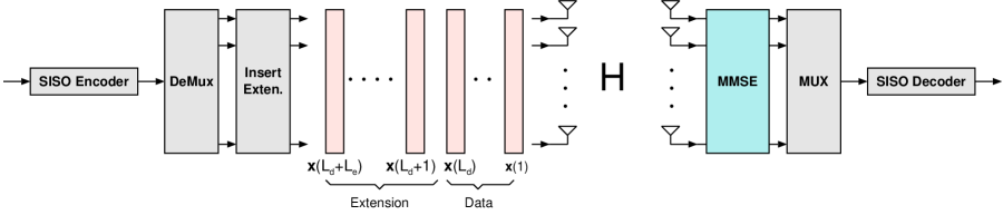
Figure 3: Single-carrier block transmission in a frequency-selective channel. In the case of CP, the extension is removed at the receiver prior to equalization.

For the single-antenna ISI channel under CP transmission, the explicit tradeoff between spectral efficiency and diversity was found [10] to be $d^{CP}_{MMSE}=1+\min(\nu,\lfloor 2^{-R}L_{d}\rfloor)$. In this section, we extend the analysis to the MIMO case. The system model is shown in Figure 3. We start with the general $M\times N$ MIMO system.

The system model is again given by (77) where ${\mathbf{H_{e}}}=\bar{\mathbf{H}}\mathbf{U_{cp}}$ and $\hat{{\mathbf{x}}}$ is generated by taking the IDFT of the information vector ${\mathbf{x}}$ [25], i.e.

$$\hat{{\mathbf{x}}}={\boldsymbol{Q}}_{Tx}^{H}{\mathbf{x}}$$ (99)

where ${\boldsymbol{Q}}_{Tx}$ is the augmented DFT matrix given by ${\boldsymbol{Q}}_{Tx}={\boldsymbol{Q}}\otimes{\mathbf{I}}_{M}$, where ${\mathbf{I}}_{M}$ is the identity matrix, ${\boldsymbol{Q}}$ is the normalized DFT matrix, and $\otimes$ is the Kroenecker product.

The $NL_{d}\times ML_{d}$ block-circulant matrix ${\mathbf{H_{e}}}$ has eigen decomposition ${\mathbf{H_{e}}}={\boldsymbol{Q}}_{Rx}^{H}{\bf{\Lambda}}{\boldsymbol{Q}}_{Tx}$, where ${\boldsymbol{Q}}_{Rx}={\boldsymbol{Q}}\otimes{\mathbf{I}}_{N}$. Both ${\boldsymbol{Q}}_{Tx}$ and ${\boldsymbol{Q}}_{Rx}$ are unitary matrices. The block diagonal matrix ${\bf\Lambda}$ is given by

$${\bf\Lambda}=\begin{pmatrix}{\bf B}_{1}&{}&{}&{0}\\ {}&{\bf B}_{2}&{}&{}\\ {}&{}&{\ddots}&{}\\ {0}&{}&{}&{\bf B}_{L_{d}}\end{pmatrix}$$ (100)

where the matrix ${\bf B}_{k}$ is given by [26]

$${\bf B}_{k}=\sum_{i=0}^{\nu}{\mathbf{H}}_{i}e^{-j\frac{2\pi i(k-1)}{L_{d}}}\quad{\text{for }}k=1,\dots,L_{d}$$ (101)

and ${\mathbf{H}}_{i}$ is the instantaneous MIMO channel (cf. Section VI-A).

Analogous to the proof of [10], we first consider the case where the transmission data-block length is equal to the number of channel taps, i.e. $L_{d}=\nu+1$. In this case, the entries of ${\mathbf{B}}_{k}{{}^{\prime}}s$ are i.i.d. normal complex Gaussian.

VI-C1 Outage upper bound

The outage probability of the MMSE receiver is given by

$$P_{out} ={\mathbb{P}}\bigg{(}\frac{1}{L_{d}}\sum_{k=1}^{ML_{d}}\log(\frac{1}{({\mathbf{I}}+\rho{\mathbf{H_{e}}}^{H}{\mathbf{H_{e}}})^{-1}_{kk}})<R\bigg{)}$$ (102)

$$={\mathbb{P}}\bigg{(}\frac{1}{L_{d}}\sum_{k=1}^{ML_{d}}\log(({\mathbf{I}}+\rho{\mathbf{H_{e}}}^{H}{\mathbf{H_{e}}})^{-1}_{kk})>-R\bigg{)}$$

$$\leqslant{\mathbb{P}}\bigg{(}M\log\sum_{k=1}^{ML_{d}}\frac{1}{ML_{d}}({\mathbf{I}}+\rho{\mathbf{H_{e}}}^{H}{\mathbf{H_{e}}})^{-1}_{kk}>-R\bigg{)}$$ (103)

$$={\mathbb{P}}\bigg{(}M\log\sum_{k=1}^{ML_{d}}\frac{1}{ML_{d}}({\mathbf{I}}+\rho{\bf\Lambda}^{H}{\bf\Lambda})^{-1}_{kk}>-R\bigg{)}$$ (104)

$$={\mathbb{P}}\bigg{(}\sum_{k=1}^{ML_{d}}({\mathbf{I}}+\rho{\bf\Lambda}^{H}{\bf\Lambda})^{-1}_{kk}>ML_{d}2^{-\frac{R}{M}}\bigg{)}$$

$$={\mathbb{P}}\bigg{(}\sum_{i=1}^{L_{d}}\text{tr}({\mathbf{I}}+\rho{\bf B}_{i}^{H}{\bf B}_{i})^{-1}>ML_{d}2^{-\frac{R}{M}}\bigg{)}$$

$$={\mathbb{P}}\bigg{(}\sum_{i=1}^{L_{d}}\sum_{k=1}^{M}\frac{1}{(1+\rho\lambda_{k,i})}>ML_{d}2^{-\frac{R}{M}}\bigg{)}$$ (105)

Where (103) follows from Jensen’s inequality, (104) follows from the eigen decomposition of ${\mathbf{H_{e}}}$, and $\lambda_{k,i}$ is $k$-th eigenvalue of the $i$-th Wishart matrix ${\bf B}_{i}^{H}{\bf B}_{i}$.

Recall from Section III that the eigenvalues of a Wishart matrix have the asymptotic property

$$\sum^{M}_{k=1}\frac{1}{1+\rho\lambda_{k}}\doteq\sum_{\alpha_{k}>1}1+\sum_{\alpha_{k}<1}\rho^{\alpha_{k}-1}$$ (106)

based on which we established in Lemmas 1 and 2 the following

$${\mathbb{P}}\big{(}\sum^{M}_{k=1}\frac{1}{1+\rho\lambda_{k}}\geqslant s\big{)}\doteq\rho^{-(s^{2}+|N-M|s)}$$ (107)

where $\alpha_{k}$ is defined in (15) and $s,M$, and $N$ are arbitrary integers. Define

$$\theta_{i}\stackrel{{\scriptstyle\triangle}}{{=}}\sum_{\alpha_{k,i}>1}1$$

$\theta_{i}$ are i.i.d. discrete random variables with the following asymptotic distribution (cf. Section III, Equations (22)-(26))

$${\mathbb{P}}\big{(}\theta_{i}=n_{i}\big{)}\doteq\rho^{-(n_{i}^{2}+|N-M|n_{i})}\quad\text{for }n_{i}=1,\dots,M$$ (108)

Using (107), the outage probability in (105) can be evaluated as

$$P_{out} \dot{\leqslant}{\mathbb{P}}\bigg{(}\sum_{i=1}^{L_{d}}\sum_{k=1}^{M}\frac{1}{(1+\rho\lambda_{k,i})}>ML_{d}2^{-\frac{R}{M}}\bigg{)}$$

$$\dot{=}{\mathbb{P}}\big{(}\sum_{i=1}^{L_{d}}\theta_{i}\geqslant\Omega\big{)}$$ (109)

where $\Omega=\lceil ML_{d}2^{-\frac{R}{M}}\rceil$. Evaluating the probability in (109) in a combinatorial manner, we get

$${\mathbb{P}}\big{(}\sum_{i=1}^{L_{d}}\theta_{i}\geqslant\Omega\big{)}\doteq{\mathbb{P}}\big{(}\sum_{i=1}^{L_{d}}\theta_{i}=\Omega\big{)}$$

$$\dot{=}\sum_{n_{1},n_{2},\dots,n_{L_{d}}}\rho^{-(n_{1}^{2}+|N-M|n_{1})}\dots\rho^{-(n_{p}^{2}+|N-M|n_{L_{d}})}$$ (110)

$$\dot{=}\max_{n_{1},n_{2},\dots,n_{L_{d}}}\rho^{-(n_{1}^{2}+|N-M|n_{1})}\dots\rho^{-(n_{L_{d}}^{2}+|N-M|n_{L_{d}})}$$ (111)

where $n_{i}\in[0,M]$ for ($i=1,2,\dots,L_{d}$) is the value of the $i$-th discrete random variable $\theta_{i}$, and (111) is true since the summation in (110) is dominated by the maximum element.

Let the set $\{n_{k}^{*},k=1,\dots,L_{d}\}$ be the set of indices of the optimal solution of (111). The set $\{n_{k}^{*}\}$ is obtained by solving the following optimization problem

$$\min_{n_{1},n_{2},\dots,n_{L_{d}}}\sum_{k=1}^{L_{d}}(n_{k}^{2}+|N-M|n_{k})$$

$$\text{subject to}\quad\quad\sum_{k=1}^{L_{d}}n_{k}=\Omega$$

$$0\leqslant n_{k}\leqslant M$$

or equivalently,

$$\min_{n_{1},n_{2},\dots,n_{L_{d}}}\quad \sum_{k=1}^{L_{d}}n_{k}^{2}$$ (112)

subject to $$\sum_{k=1}^{L_{d}}n_{k}=\Omega$$

$$n_{k}\geq 0$$

The problem in (112) is a quadratic integer-programming (QIP) problem (see e.g. [27] ). Integer programming problems are in general NP-hard. However, due to the simple structure of the objective function in (112), we can efficiently solve it, thus obtain a closed form expression for $\{n_{k}^{*}\}$ and hence (111).

Lemma 8

For the QIP given by (112), the optimum solution is given by:

$$n_{i}^{*}=u\quad\text{for }1\leqslant i\leqslant t$$

$$n_{j}^{*}=u+1\quad\text{for }t+1\leqslant j\leqslant L_{d}$$

where $u=\lfloor\frac{\Omega}{L_{d}}\rfloor$ and $t=L_{d}(u+1)-\Omega$.

Proof:

See Appendix -B ∎

Using Lemma 8, we can now evaluate the outage upper bound given by (111) as

$$P_{out}\hskip 4.0pt\dot{\leqslant}\hskip 4.0pt\rho^{-d_{cp}}$$ (113)

where $d_{cp}=\Omega(2u+1)-uL_{d}(u+1)+|N-M|\Omega$ and $u=\lfloor\frac{\Omega}{L_{d}}\rfloor$.

VI-C2 Outage lower bound

The bound is obtained using the same steps to obtain the lower bound in Section VI-B1. It can be shown that

$$P_{out} ={\mathbb{P}}\bigg{(}\frac{1}{L_{d}}\sum_{k=1}^{ML_{d}}\log(({\mathbf{I}}+\rho{\mathbf{H_{e}}}^{H}{\mathbf{H_{e}}})^{-1}_{kk})>-R\bigg{)}$$ (114)

$$\dot{\geqslant}\hskip 5.0pt{\mathbb{P}}\bigg{(}\sum_{i=1}^{L_{d}}\sum_{k=1}^{M}\frac{1}{(1+\rho\lambda_{k,i})}>ML_{d}2^{-\frac{R}{M}}\bigg{)}$$ (115)

The bound in (115) is the same as the upper bound in (105), thus the bound is tight and the diversity is given by (113). The PEP analysis follows in a manner similar to Section IV.

Recall that so far we have considered data block length $L_{d}=\nu+1$. It can be shown that the diversity for any $L_{d}>\nu+1$ is upper bounded by the computed diversity for the case $L_{d}=\nu+1$. This bounding is derived from (104) via FFT arguments similar to those used in [10], which we omit for brevity. A tight diversity lower bound for data block lengths $L_{d}>\nu+1$ remains an open problem, except for the SIMO system as discussed in the next section.

VI-C3 Diversity of CP Transmission in the SIMO Channel

Theorem 5

In a SIMO quasi-static frequency-selective channel with memory $\nu$, $N$ receive antennas and data-block length $L_{d}$, the MMSE receiver diversity is $d^{CP}_{MMSE}=N\min(\nu+1,\lfloor 2^{-R}L_{d}\rfloor+1)$ under joint spatial encoding and cyclic prefix transmission.

In order to prove Theorem 5, we first analyze the case of $L_{d}=\nu+1$ and then generalize the result for $L_{d}>\nu+1$. The system model is given by (77) where the $NL_{d}\times L_{d}$ equivalent channel matrix is given by

$${\mathbf{H_{e}}}=\begin{bmatrix}{\mathbf{h}}_{0}&{\mathbf{h}}_{1}&\cdots&{\mathbf{h}}_{\nu}&0&\cdots&0\\ 0&{\mathbf{h}}_{0}&{\mathbf{h}}_{1}&\cdots&{\mathbf{h}}_{\nu}&\cdots&0\\ \vdots&\ddots&\ddots&\ddots&\ddots&\ddots&\vdots\\ {\mathbf{h}}_{1}&{\mathbf{h}}_{2}&\cdots&{\mathbf{h}}_{\nu}&0&\cdots&{\mathbf{h}}_{0}\end{bmatrix}.$$ (116)

where ${\mathbf{h}}_{i}$ (for $i=0,1,\dots,\nu$) is $N\times 1$ SIMO channel. Note that the diagonal elements of (${\mathbf{H_{e}}}^{H}{\mathbf{H_{e}}}$) are identical and equal to $\sum_{i=0}^{\nu}{\mathbf{h}}_{i}^{H}{\mathbf{h}}_{i}$. Thus the MMSE SINR for each output information stream is

$$\gamma_{k}=\frac{1}{({\mathbf{I}}+{\mathbf{H_{e}}}^{H}{\mathbf{H_{e}}})_{kk}}-1=\frac{1}{\frac{1}{L_{d}}\text{tr}({\mathbf{I}}+{\mathbf{H_{e}}}^{H}{\mathbf{H_{e}}})_{kk}}-1$$ (117)

Evaluating the outage probability as in (102)

$$P_{out} ={\mathbb{P}}\bigg{(}\frac{1}{L_{d}}\sum_{k=1}^{L_{d}}\log(\frac{1}{({\mathbf{I}}+\rho{\mathbf{H_{e}}}^{H}{\mathbf{H_{e}}})^{-1}_{kk}})<R\bigg{)}$$

$$={\mathbb{P}}\bigg{(}\log\frac{1}{L_{d}}\sum_{k=1}^{L_{d}}\frac{1}{({\mathbf{I}}+\rho{\mathbf{H_{e}}}^{H}{\mathbf{H_{e}}})^{-1}_{kk}}<R\bigg{)}$$ (118)

$$={\mathbb{P}}\bigg{(}\sum_{k=1}^{L_{d}}\frac{1}{(1+\rho\lambda_{k})}>L_{d}2^{-R}\bigg{)}$$ (119)

where (118) follows from (117) and (119) follows similarly to (105).

In a manner similar to (105) we have $\lambda_{k}={\bf B}_{k}^{H}{\bf B}_{k}$ because now $\mathbf{B}$ is simply a $N\times 1$ vector. For the case $L_{d}=\nu+1$, the eigenvalues $\{\lambda_{k}\}$ are distributed according to Gamma distribution with shape parameter $N$ and scale parameter $1$, i.e. $\lambda_{k}\sim{\Gamma}(N,1)$. For $L_{d}>\nu+1$ the Gaussian variables in ${\mathbf{B}}_{k}$ are no longer independent and thus analyzing this case requires the unknown distribution $\{\lambda_{k}\}$. Instead, we indirectly show that the diversity of $L_{d}=\nu+1$ also holds for $L_{d}>\nu+1$.

Lemma 9

In a SIMO quasi-static frequency-selective channel with memory $\nu$, $N$ receive antennas and data-block length $L_{d}=\nu+1$, the MMSE receiver diversity is $d^{CP}_{MMSE}={N(\lfloor L_{d}2^{-R}\rfloor+1)}$ under joint spatial encoding and cyclic prefix transmission.

Proof:

The outage probability can be written as

$$P_{out} ={\mathbb{P}}\big{(}\sum_{k=1}^{L_{d}}\frac{1}{(1+\rho\lambda_{k})}>L_{d}2^{-R}\big{)}$$

$$\dot{=}\hskip 6.0pt{\mathbb{P}}\big{(}M({\mathbf{\alpha}})>L_{d}2^{-R}\big{)}$$ (120)

where we use $M({\mathbf{\alpha}})=\sum_{\alpha_{k}>1}1$ from (106). We thus need to evaluate ${\mathbb{P}}(\alpha>1)$. The probability density function of $\lambda_{k}$ is

$$f_{\lambda_{k}}(x)=\frac{1}{\Gamma(N)}\,x^{N-1}\,e^{-x}$$ (121)

The distribution of $\alpha_{k}$ is thus given by

$$f_{\alpha_{k}}(x)=\frac{1}{\Gamma(N)}\,\rho^{-Nx}\,e^{-x}\,\ln{\frac{1}{\rho}}$$ (122)

The cumulative distribution function of $\alpha_{k}$ is

$$F_{\alpha_{k}}(x) =\int_{-\infty}^{x}f_{\alpha_{k}}(y)\;dy$$

$$=\frac{1}{\Gamma(N)}\int_{\rho^{-x}}^{\infty}r^{N-1}e^{-r}dr$$ (123)

$$=\frac{1}{\Gamma(N)}\bigg{(}\int_{0}^{\infty}r^{N-1}e^{-r}dr-\int_{0}^{\rho^{-x}}r^{N-1}e^{-r}dr\bigg{)}$$ (124)

$$=e^{-\rho^{-\alpha}}\sum_{k=0}^{N-1}\frac{\rho^{-xk}}{k!}$$ (125)

where we have made a change of variables $r=\rho^{-x}$ in (123), and evaluate the integral according to [24, P.334 and P.336]. Thus we have

$$P(\alpha_{k}>1) =1-e^{-\rho}\sum_{k=0}^{N-1}\frac{\rho^{-k}}{k!}$$

$$\doteq 1-\big{(}1-\frac{1}{N!}\rho^{-N}\big{)}$$ (126)

$$\doteq\rho^{-N}$$ (127)

where (126) follows from the Taylor expansion for (125).

From the independence of $\{\lambda_{k}\}$, and subsequently the independence of $\{\alpha_{k}\}$, we conclude that $M({\mathbf{\alpha}})$ in (120) is binomially distributed with parameter $\rho^{-N}$. Hence, similar to [10], we have

$${\mathbb{P}}\bigg{(}\sum_{k=1}^{L_{d}}\frac{1}{1+\rho\lambda_{k}}>L_{d}2^{-R}\bigg{)}\doteq{\mathbb{P}}(M(\alpha)>L_{d}2^{-R})$$

$$=\sum_{i=\lfloor L_{d}2^{-R}\rfloor+1}^{L_{d}}{\mathbb{P}}(M(\alpha)=i)$$

$$\doteq\sum_{i=\lfloor L_{d}2^{-R}\rfloor+1}^{L_{d}}\begin{pmatrix}{L_{d}}\\ {i}\end{pmatrix}\rho^{-Ni}\underbrace{(1-\rho^{-N})^{n-i}}_{\doteq 1}$$

$$\doteq\rho^{-N{(\lfloor L_{d}2^{-R}\rfloor+1)}}.$$

which concludes the proof for $L_{d}=\nu+1$ ∎

For $L_{d}>\nu+1$ we follow steps similar to [10].

Lemma 10

Consider two SIMO systems both operating under quasi-static frequency-selective channels with memory $\nu$. One system has data block length $L_{d_{1}}>\nu+1$ and the other $L_{d_{2}}\geq L_{d_{1}}$, we have the following property

$${\mathbb{P}}\bigg{(}\sum_{k=1}^{L_{d_{1}}}\frac{1}{(1+\rho\lambda_{k})}>m\bigg{)}\doteq{\mathbb{P}}\bigg{(}\sum_{k=1}^{L_{d_{2}}}\frac{1}{(1+\rho\lambda_{k})}>m\bigg{)}$$

for any $m\in\mathbb{R}$.

Proof:

The proof has similarities with the SISO case developed in [10, Lemma 2], but is not a trivial extension (see Appendix -C). ∎

Using Lemma 10 and the results in [10, Theorem 2], Theorem 5 is established.

VII Simulation Results

Simulations generate Monte Carlo random channel realizations and calculate outage probability by checking the appropriate linear MIMO receiver mutual information for the quasi-static flat fading model. Figure 4 shows the case $M=N=3$. According to Theorem 2, $d_{out}=1$ for $R\geqslant 4.755$, $d_{out}=4$ for $4.755>R\geqslant 1.755$, and $d_{out}=9$ for $R<1.7549$. Figure 4 shows the diversity step between $R=4.5$ and $4.8$bps/Hz. The slope of diversity 9 is difficult to measure precisely with simulations, but it is approximately observed. Figure 5 shows the outage probability for $R=1,4\text{ and }10$ with the Jensen bound, with a diversity transition at $R=2$. Figure 6 shows the case of $M=2,\text{ and }N=3$ again with transition at $R=2$. In Figure 7, simulations results for $N=2$ and $M=3$ are given and compared with $N=3$ and $M=2$. Theorem 2 gives the diversity for both systems. It is observed that when $N>M$ the break point of the slopes occurs before its counterparts in $M>N$ case. Lower rates were difficult to simulate precisely.

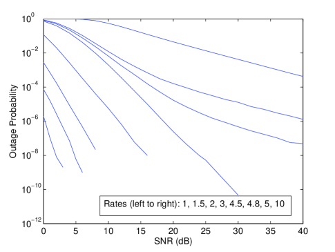
Figure 4: Outage probability of MMSE Receiver, $M=N=3$ for R=1, 1.5, 2, 3, 4.5, 4.8, 5, 10 bps/Hz

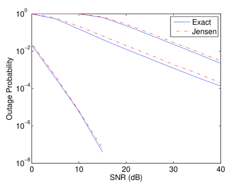
Figure 5: Outage probability of MMSE Receiver, $M=N=2$ for R (left to right)= 1, 4, 10 bps/Hz

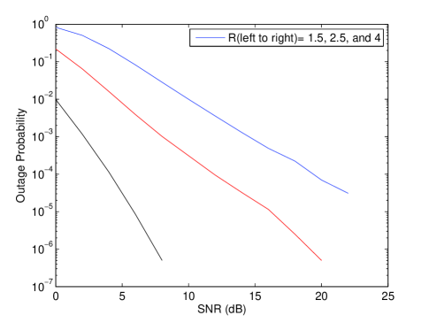
Figure 6: Outage probability of MMSE Receiver, $M=2,\text{ and }N=3$ for R (left to right)= 1.5, 2.5, 4 bps/Hz

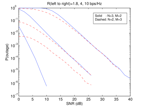
Figure 7: Outage probability of MMSE Receiver for both cases $N>M$ (solid) and $M>N$ (dashed). The spectral efficiency $R$ (left to right)= 1.8, 4, and 10 bps/Hz

VIII Conclusion

This paper settles the long standing problem of the diversity of the MMSE MIMO receivers under all fixed rates for any number of transmit ($M$) and receive ($N$) antennas, giving the result as $d=\lceil M2^{-\frac{R}{M}}-(M-N)^{+}\rceil^{2}+|N-M|\lceil M2^{-\frac{R}{M}}-(M-N)^{+}\rceil$. The analysis confirms the earlier approximate results [6, 7] showing that the system diversity can be as high as $MN$ for low spectral efficiency and as low as $N-M+1$ for high spectral efficiency. The result is extended to the multiple access channel (MAC). We also analyze the case of frequency-selective MIMO channel under cyclic-prefix and zero-padding transmission, and obtain the explicit tradeoff between rate and diversity.

-A Proof of Lemma 5

Consider a single-antenna ISI channel $\mathbf{h}=[h_{0},\dots,h_{\nu}]$, where $\nu$ is channel memory. The transmitter sends a block of $L_{d}+\nu$ symbols (i.e. the extension $L_{e}=\nu$), the last $\nu$ symbols of which are zeros to remove the inter-block interference. The system model is given by

$${\mathbf{y}}=\mathbf{{\mathbf{H_{e}}}}{\mathbf{x}}+{\mathbf{n}}$$ (128)

where ${\mathbf{x}}$ is the transmitted length-$(L_{d}+\nu)$ vector. We consider the case where the padding length is equal to the memory of the channel. The results are also valid for $L_{e}>\nu$ as a direct result of [10, Theorem 2].

The outage probability of MMSE receiver under ZP transmission is given by [10]

$$P_{out} ={\mathbb{P}}\big{(}\frac{1}{L_{d}}\sum_{k=1}^{L_{d}}\log(\frac{1}{({\mathbf{I}}+\rho{\mathbf{H_{e}}}^{H}{\mathbf{H_{e}}})^{-1}_{kk}})<R\big{)}$$

$$\leqslant{\mathbb{P}}\big{(}\frac{1}{L_{d}}\sum_{k=1}^{L_{d}}\log(1+\frac{\rho}{({\mathbf{H_{e}}}^{H}{\mathbf{H_{e}}})^{-1}_{kk}})<R\big{)}$$ (129)

$$\leqslant{\mathbb{P}}\big{(}\log\frac{1}{L_{d}}\sum_{k=1}^{L_{d}}\frac{1}{\rho}({\mathbf{H_{e}}}^{H}{\mathbf{H_{e}}})^{-1}_{kk}>-R\big{)}$$ (130)

$$={\mathbb{P}}\big{(}\frac{L_{d}\hskip 2.0pt2^{-R}}{\text{tr}({\mathbf{H_{e}}}^{H}{\mathbf{H_{e}}})^{-1}}<\rho^{-1}\big{)}$$ (131)

where (129) represents the outage probability of zero-forcing equalizer which upper bounds that of the MMSE. The bound in (130) follows from Jensen’s inequality.

We want to show that ${\text{ tr}}({\mathbf{H_{e}}}^{H}{\mathbf{H_{e}}})^{-1}$ in (131) is proportional to $||{\bf h}||^{-2}$. Thus it is straightforward to obtain full-diversity at any $R$ since [15]

$${\mathbb{P}}\big{(}c\hskip 2.0pt||{\bf h}||^{2}<\rho^{-\alpha}\big{)}\dot{=}\rho^{-L\alpha}$$ (132)

where $c$ is a constant that is independent of ${\bf h}$.

To show that this is indeed the case, we use the result of Tepedelenlioglu [22, 28] which provides a family of linear zero-forcing equalizers that is capable of achieving full multipath diversity in zero-padded systems under certain constraints. We paraphrase the result for convenience.

Lemma 11 ([22, 28])

Under zero-padded transmission, there exists a family of left-inverses of ${\mathbf{H_{e}}}$, denoted by ${\bf G}$, such that $||{\bf G}||^{-2}\geqslant C||{\mathbf{h}}||^{2}$ for some constant $C$ independent of the channel vector ${\mathbf{h}}$. Moreover, we have $||{\mathbf{W}}_{ZF}||\leqslant||{\bf G}||$, for any ${\bf G}$ satisfying ${\bf G}{\mathbf{H_{e}}}={\mathbf{I}}$, and ${\mathbf{W}}_{ZF}$ is given by

$${\mathbf{W}}_{ZF}=({\mathbf{H_{e}}}^{H}{\mathbf{H_{e}}})^{-1}{\mathbf{H_{e}}}^{H}.$$ (133)

Applying the ZF equalizer ${\mathbf{W}}_{ZF}$ on the channel output given by (128) we get the equalized signal $\tilde{{\mathbf{y}}}={\mathbf{x}}+{\mathbf{z}}$, where ${\mathbf{z}}={\mathbf{W}}_{ZF}{\mathbf{n}}$. The filtered noise power $P_{z}$ can be evaluated as

$$P_{z} ={\mathbb{E}}\hskip 2.0pt\text{tr}[{\mathbf{z}}{\mathbf{z}}^{H}]$$

$$=\text{tr}\big{[}{\mathbb{E}}(({\mathbf{H_{e}}}^{H}{\mathbf{H_{e}}})^{-1}{\mathbf{H_{e}}}^{H}{\mathbf{n}}{\mathbf{n}}^{H}{\mathbf{H_{e}}}({\mathbf{H_{e}}}^{H}{\mathbf{H_{e}}})^{-1})\big{]}$$

$$=\text{tr}[({\mathbf{H_{e}}}^{H}{\mathbf{H_{e}}})^{-1}]$$ (134)

where we assume the noise is uncorrelated and has variance equal to one.

Using the properties of the Frobenius norm, $P_{z}$ can be bounded as

$$P_{z} ={\mathbb{E}}(||{\mathbf{W}}_{zf}{\mathbf{n}}||^{2})$$

$$\leqslant{\mathbb{E}}(||{\mathbf{W}}_{zf}||^{2}||{\mathbf{n}}||^{2})=L_{d}||{\mathbf{W}}_{zf}||^{2}.$$ (135)

Using (134), (135) and Lemma 11, the trace in (131) can be bounded by

$$\text{tr}[({\mathbf{H_{e}}}^{H}{\mathbf{H_{e}}})^{-1}]\leqslant L_{d}||{\mathbf{W}}_{zf}||^{2}\leqslant\frac{L_{d}}{C\hskip 2.0pt||{\bf h}||^{2}}.$$ (136)

Thus from (131) we have

$$P_{out} \dot{\leqslant}{\mathbb{P}}\big{(}C_{2}||{\bf h}||^{2}<\rho^{-1}\big{)}$$

$$\dot{=}\quad\rho^{-(\nu+1)}.$$ (137)

where $C_{2}=C\;2^{-R}$ is a constant independent of ${\mathbf{h}}$ and $\rho$.

Note that the constraints and construction methods in [22, 28] for the zero-forcing equalizers to achieve full multipath diversity in ZP systems do not apply in CP systems. That is, Lemma 11 is not true for CP transmission. This is because the equivalent channel in CP systems does not have the same properties that were used in [22, 28].

-B Proof of Lemma 8:(QIP Problem)

Consider the following Quadratic Integer Programming (QIP) problem

$$\min_{n_{1},n_{2},\dots,n_{\ell}}\quad \sum_{k=1}^{\ell}n_{k}^{2}$$ (138)

subject to $$\sum_{k=1}^{\ell}n_{k}=\Omega$$

$$n_{k}\geq 0.$$

where $\Omega$ and $\ell$ are integers.

Consider a candidate solution vector $[n_{1},\ldots,n_{k},\ldots,n_{\ell}]$. We partition the variables in this vector according to their values into $\Omega+1$ sets $\mathcal{N}_{j}=\{n_{k}:n_{k}=j\}$ for $0\leq j\leq\Omega$; clearly some of these sets may be empty. Denote the membership of each set $S_{j}=|\mathcal{N}_{j}|$. Furthermore, let $\Omega=m\ell+K$ where $m$ is the divisor and $K$ is the remainder of the division of $\Omega$ by $\ell$. From the constraint in (138) we have

$$\sum_{k=1}^{\ell}n_{k}=\sum_{j=0}^{\Omega}jS_{j}=m\ell+\sum_{j=0}^{\Omega}(j-m)S_{j}=m\ell+K.$$ (139)

Evaluating the objective function:

$$\sum_{k=1}^{\ell}n_{k}^{2} =\sum_{j=0}^{\Omega}(m+j-m)^{2}S_{j}$$

$$=\ell m^{2}+2m\sum_{j=0}^{\Omega}(j-m)S_{j}+\sum_{j=0}^{\Omega}(j-m)^{2}S_{j}$$

$$=\ell m^{2}+2mK+\sum_{j=0}^{\Omega}(j-m)^{2}S_{j}$$ (140)

$$\geqslant\ell m^{2}+2mK+\sum_{j=0}^{\Omega}(j-m)S_{j}$$ (141)

$$=\ell m^{2}+2mK+K$$ (142)

where (140) and (142) use $\sum_{j=0}^{\Omega}(j-m)S_{j}=K$, which follows from (139).

We now propose that one may achieve optimality when all variables take values either $m$ or $m+1$. In that case,

$$\sum_{k}n_{k} =mS_{m}+(m+1)(\ell-S_{m})=m\ell+(\ell-S_{m})$$

$$\sum_{k}n_{k}^{2} =m^{2}S_{m}+(m+1)^{2}(\ell-S_{m})=\ell m^{2}+2mK+K.$$

where we substituted the value of $\ell-S_{m}$ from the first equation into the second equation above. This shows that the variables taking values $m$ or $m+1$ achieves the lower bound in (142). At optimality $S_{m}=(m+1)\ell-\Omega$.

-C Proof of Lemma 10

We begin by showing that for any integer multiplier of $L_{d_{1}}=\nu+1$ denoted by $L_{d_{2}}=TL_{d_{1}}$ ($T\in\mathbb{N}$) and any real-valued $m\in(0,L_{d_{1}})$, we have

$${\mathbb{P}}\bigg{(}\sum_{q=1}^{L_{d_{1}}}\frac{1}{(1+\rho\lambda_{q})}>m\bigg{)}\doteq{\mathbb{P}}\bigg{(}\sum_{q=1}^{L_{d_{2}}}\frac{1}{(1+\rho\lambda_{q})}>m\bigg{)}$$ (143)

Note that for SIMO-CP system, $\lambda_{q}={\mathbf{b}}_{q}^{H}{\mathbf{b}}_{q}$, where ${\mathbf{b}}_{q}$ is the $N\times 1$ vector given by

$${\mathbf{b}}^{(i)}_{q}=\sum_{n=0}^{\nu}{\mathbf{h}}_{n}\,e^{-j\frac{2\pi(q-1)}{L_{d_{i}}}}\quad{\text{for }}q=1,\dots,L_{d_{i}}$$ (144)

where ${\mathbf{h}}_{n}$ is the channel gain as a function of the tap index $n$, and the superscript $i=1,2$ is used to distinguish the variables in two systems with data block lengths $L_{d_{1}}$ and $L_{d_{2}}$.

Recall that we can take a $L_{d_{1}}$-point signal and apply a $L_{d_{2}}$-point DFT on it (after zero-padding), which will result in a resampling in the Fourier domain at $L_{d_{2}}$ points. Following [10] we can write the explicit relationship between entries of ${\mathbf{b}}^{(1)}$ and ${\mathbf{b}}^{(2)}$ as

$${b}^{(1)}_{q,l}=\sum_{i=1}^{L_{d_{1}}}{b}^{(2)}_{i,l}\psi_{i}\quad q=1,2\dots,L_{d_{2}}\text{ and }l=1,2,\dots,N.$$ (145)

where

$$\psi_{i}=\frac{1}{L_{d_{1}}}\frac{1-e^{-j\frac{(q-1)2\pi L_{d_{1}}}{L_{d_{2}}}}}{1-e^{-j\big{(}\frac{2\pi(q-1)}{L_{d_{2}}}-\frac{2\pi(i-1)}{L_{d_{1}}}\big{)}}}.$$

Define $\alpha^{(i)}_{q,l}=\-\frac{\log{|b^{(i)}_{q,l}|^{2}}}{\log{\rho}}$. Note that $b^{(1)}_{T(q-1),l}=b^{(2)}_{q,l}$ and $\alpha^{(2)}_{T(q-1),l}=\alpha^{(1)}_{q,l}$ for $q=1,2\dots,L_{d_{1}}$ since $L_{d_{2}}=TL_{d_{1}}$ . From (145), we have

$$|{b}^{(1)}_{q,l}|^{2}=\sum_{i=1}^{L_{d_{1}}}|\psi_{i}|^{2}|{b}^{(2)}_{i,l}|^{2}+\underbrace{\sum_{i=1}^{L_{d_{1}}}\sum_{s=1}^{L_{d_{1}}}\psi_{i}\psi_{s}{b}^{(2)}_{i,l}{b}^{*(2)}_{s,l}}_{\triangleq\,\,\eta}.$$ (146)

We now analyze each part of the sum in (146). For the set of indices $\mathcal{A}\triangleq\{i:i=T(k-1)+1,k=1,\dots,L_{d_{1}}\}$, the coefficients $\{\psi_{i}\}$ are non-zero constants, then $|\psi_{i}|^{2}|b^{(2)}_{i,l}|^{2}\doteq|b^{(2)}_{i,l}|^{2}\quad\forall l$. Noting that $\eta$ must be real-valued, and defining $\alpha_{\eta}\triangleq-\frac{\log{|\eta|}}{\log\rho}$, Eq. (146) can be written as

$$\rho^{-\alpha^{(2)}_{q,l}} \dot{=}\sum_{i=1}^{L_{d_{1}}}\rho^{-\alpha^{(1)}_{i,l}}+\frac{\eta}{|{\eta}|}\rho^{-\alpha_{\eta}}$$

$$\dot{=}\rho^{-\min_{i}\alpha^{(1)}_{i,l}}+\frac{\eta}{|{\eta}|}\rho^{-\alpha_{\eta}}.$$ (147)

Note that if $\eta<0$ the second term in (147) should be smaller than the first term since otherwise the right-hand side of (147) will be negative while the left-hand side is positive. Thus for $\eta<0$ we have $\alpha_{\eta}\geqslant\min_{i}\alpha^{(1)}_{i.l}$. Also, for $a\geqslant 0$ we have $\rho^{-\min_{i}\alpha^{(1)}_{i,l}}+\frac{\eta}{|{\eta}|}\rho^{-\alpha_{\eta}}\dot{\geqslant}\rho^{-\min_{i}\alpha^{(1)}_{i,l}}$. Thus we always have $\rho^{-\min_{i}\alpha^{(1)}_{i,l}}+\frac{\eta}{|{\eta}|}\rho^{-\alpha_{\eta}}\dot{\geqslant}\rho^{-\min_{i}\alpha^{(1)}_{i,l}}$, leading to the following lemma.

Lemma 12

For $\alpha^{(1)}_{q,l}$ and $\alpha^{(2)}_{q,l}$ defined above we have: $\rho^{-\alpha^{(2)}_{q,l}}\dot{\geqslant}\rho^{-\min_{i}{\alpha^{(1)}_{i,l}}}\Rightarrow\alpha^{(2)}_{q,l}\leqslant{\min_{i}{\alpha^{(1)}_{i,l}}}$ for $q\in\mathcal{A}$.

We now partition the DFT points into two sets $\mathcal{A}=\{T(i-1)+1,i=1,\dots,L_{d_{1}}\}$ and $\mathcal{B}=\{1,\dots,L_{d_{2}}\}\backslash\{T(i-1)+1,i=1,\dots,L_{d_{1}}\}$ We now define the event:

$$\mathcal{D}\stackrel{{\scriptstyle\triangle}}{{=}}\{\min_{i}\alpha^{(1)}_{i,1}<1\;,\;\min_{i}\alpha^{(1)}_{i,2}<1\;,\;\dots\;,\;\min_{i}\alpha^{(1)}_{i,N}<1\}$$

and proceed to evaluate the probability

$${\mathbb{P}}\bigg{(}\sum_{q=1}^{L_{d_{2}}}\frac{1}{(1+\rho\lambda_{q})}>m\bigg{)}={\mathbb{P}}\bigg{(}\sum_{q=1}^{L_{d_{2}}}\frac{1}{1+\rho\sum_{l=1}^{N}|b^{(1)}_{q,l}|^{2}}>m\bigg{)}$$ (148)

$$={\mathbb{P}}\bigg{(}\sum_{q\in{\mathcal{A}}}\frac{1}{1+\rho\sum_{l=1}^{N}|b^{(1)}_{q,l}|^{2}}+\sum_{q\in\mathcal{B}}\frac{1}{1+\rho\sum_{l=1}^{N}|b^{(1)}_{q,l}|^{2}}>m\bigg{)}$$

$$\doteq{\mathbb{P}}\bigg{(}S_{1}+S_{2}>m\bigg{)}$$ (149)

where (148) follows since $\lambda_{q}={\mathbf{b}}_{q}^{H}{\mathbf{b}}_{q}$ and $S_{1}$ and $S_{2}$ are given by

$$S_{1} \triangleq\sum_{q=1}^{L_{d_{1}}}\frac{1}{1+\sum_{l=1}^{N}\rho^{1-\alpha^{(1)}_{q,l}}}$$

$$S_{2} \triangleq\sum_{q\in\mathcal{B}}\frac{1}{1+\sum_{l=1}^{N}\rho^{1-\alpha^{(2)}_{q,l}}}$$

We now evaluate (149)

$${\mathbb{P}}\bigg{(}S_{1}+S_{2}>m\bigg{)}={\mathbb{P}}\bigg{(}S_{1}+S_{2}>m\;\bigg{|}\;\mathcal{D}\bigg{)}\times{\mathbb{P}}(\mathcal{D})\;+$$

$$\hskip 100.0pt{\mathbb{P}}\bigg{(}S_{1}+S_{2}>m\;\bigg{|}\;\bar{\mathcal{D}}\bigg{)}\times{\mathbb{P}}(\bar{\mathcal{D}})$$ (150)

Note that subject to the event $\mathcal{D}$, we have

$$S_{2}=\sum_{q\in\mathcal{B}}\frac{1}{1+\sum_{l=1}^{N}\rho^{1-\alpha^{(2)}_{q,l}}}\doteq 0$$

Therefore this term can be asymptotically ignored. Also subject to $\bar{\mathcal{D}}$, we have

$$S_{1}=\sum_{q=1}^{L_{d_{1}}}\frac{1}{1+\sum_{l=1}^{N}\rho^{1-\alpha^{(1)}_{q,l}}}\doteq L_{d_{1}}$$

and since with probability one, $L_{d_{1}}\geq m$, the other (non-negative) term can be asymptotically ignored. Thus, both the terms involving the set $\mathcal{B}$ can be altogether ignored and we have:

$${\mathbb{P}}\bigg{(}\sum_{q=1}^{L_{d_{2}}}\frac{1}{(1+\rho\lambda_{q})}>m\bigg{)} \doteq{\mathbb{P}}\bigg{(}S_{1}>m|\mathcal{D}\bigg{)}{\mathbb{P}}(\mathcal{D})+$$

$$\qquad{\mathbb{P}}\bigg{(}S_{1}>m|\bar{\mathcal{D}}\bigg{)}{\mathbb{P}}(\bar{\mathcal{D}})$$

$$\doteq{\mathbb{P}}\bigg{(}\sum_{q=1}^{L_{d_{1}}}\frac{1}{(1+\rho\lambda_{q})}>m\bigg{)}$$

We have thus established  (143) when $L_{d_{1}}|L_{d_{2}}$. We must now show that the same result holds for any $T^{\prime}$ when $L_{d_{1}}\nmid T^{\prime}$. To do so, let $L_{d_{2}}=T{{}^{\prime}}L_{d_{1}}$, then we have

$${\mathbb{P}}\bigg{(}\sum_{q=1}^{L_{d_{2}}}\frac{1}{(1+\rho\lambda_{q})}>m\bigg{)}\doteq{\mathbb{P}}\bigg{(}\sum_{q=1}^{T{{}^{\prime}}}\frac{1}{(1+\rho\lambda_{q})}>m\bigg{)}.$$ (151)

Using (143) when $L_{d_{1}}|L_{d_{2}}$ and (151) when $T{{}^{\prime}}|L_{d_{2}}$ together establishes (143) for any two positive integers.

References

- [1] P. Li, D. Paul, R. Narasimhan, and J. Cioffi, “On the distribution of SINR for the MMSE MIMO receiver and performance analysis,” IEEE Trans. Inform. Theory, vol. 52, no. 1, pp. 271–286, Jan. 2006.
- [2] A. L. Moustakas, K. R. Kumar, and G. Caire, “Performance of MMSE MIMO receivers: A large n analysis for correlated channels,” in Proc. IEEE Vehicular Technology Conference (VTC), Apr. 2009, pp. 1–5.
- [3] E. A. Jorswieck and H. Boche, “Information theory outage probability in multiple antenna system,” European Trans. on Telecommun., vol. 18, no. 3, pp. 217–233, June 2006.
- [4] Y. Jiang, M. Varanasi, and J. Li, “Performance analysis of ZF and MMSE equalizers for MIMO systems: An In-Depth study of the high SNR regime,” IEEE Trans. Inform. Theory, vol. 57, no. 4, pp. 2008–2026, Apr. 2011.
- [5] E. N. Onggosanusi, A. G. Dabak, T. Schmidl, and T. Muharemovic, “Capacity analysis of frequency-selective MIMO channels with sub-optimal detectors,” in Proc. IEEE ICASSP, vol. 3, May 2002, pp. 2369–2372.
- [6] A. Hedayat and A. Nosratinia, “Outage and diversity of linear receivers in flat-fading MIMO channels,” IEEE Trans. Signal Processing, vol. 55, no. 12, pp. 5868–5873, Dec. 2007.
- [7] K. R. Kumar, G. Caire, and A. L. Moustakas, “Asymptotic performance of linear receivers in MIMO fading channels,” IEEE Trans. Inform. Theory, vol. 55, no. 10, pp. 4398–4418, Oct. 2009.
- [8] H. Gao, P. J. Smith, and M. V. Clark, “Theoretical reliability of MMSE linear diversity combining in rayleigh-fading additive interference channels,” IEEE Trans. Commun., vol. 46, no. 5, pp. 666–672, May 1998.
- [9] D. Gore, A. Gorokhov, and A. Paulraj, “Joint MMSE versus v-BLAST and antenna selection,” in Proc. Asilomar Conference on Signals, Systems and Computers, vol. 1, Nov. 2002, pp. 505–509.
- [10] A. Tajer and A. Nosratinia, “Diversity order in ISI channels with single-carrier frequency-domain equalizer,” IEEE Trans. Wireless Commun., vol. 9, no. 3, pp. 1022 –1032, Mar. 2010.
- [11] S. Verdú, Multiuser Detection. Cambridge University Press, 1998.
- [12] I. E. Telatar, “Capacity of multi-antenna gaussian channels,” European Trans. on Telecommun., vol. 10, pp. 585–595, Nov./Dec. 1999.
- [13] A. James, “Distributions of matrix variates and latent roots derived from normal samples,” Annals of Mathematical Statistics, vol. 35, pp. 475–501, 1964.
- [14] D. Tse and P. Viswanath, Fundamentals of Wireless Communication. Cambridge University Press, 2005.
- [15] L. Zheng and D. N. C. Tse, “Diversity and multiplexing: a fundamental tradeoff in multiple-antenna channels,” IEEE Trans. Inform. Theory, vol. 49, no. 5, pp. 1073–1096, May 2003.
- [16] T. M. Cover and J. A. Thomas, Elements of Information Theory. John Wiley and Sons, 1991.
- [17] N. Al-Dhahir, “Single-carrier frequency-domain equalization for space-time block-coded transmissions over frequency-selective fading channels,” IEEE Commun. Lett., vol. 5, no. 7, pp. 304 –306, July 2001.
- [18] H. Sari, G. Karam, and I. Jeanclaude, “Transmission techniques for digital terrestrial tv broadcasting,” IEEE Commun. Mag., vol. 33, no. 2, pp. 100 –109, Feb. 1995.
- [19] B. Muquet, Z. Wang, G. Giannakis, M. de Courville, and P. Duhamel, “Cyclic prefixing or zero padding for wireless multicarrier transmissions?” IEEE Trans. Commun., vol. 50, no. 12, pp. 2136 – 2148, Dec. 2002.
- [20] Z. Wang, X. Ma, and G. Giannakis, “Optimality of single-carrier zero-padded block transmissions,” in Proc. IEEE Wireless Communcations and Networking Conference (WCNC), vol. 2, Mar. 2002, pp. 660 – 664.
- [21] A. Scaglione, P. Stoica, S. Barbarossa, G. Giannakis, and H. Sampath, “Optimal designs for space-time linear precoders and decoders,” IEEE Trans. Signal Processing, vol. 50, no. 5, pp. 1051 –1064, May 2002.
- [22] C. Tepedelenlioglu, “Low complexity linear equalizers with maximum multipath diversity for zero-padded transmissions,” in Proc. IEEE ICASSP, vol. 4, apr 2003, pp. 636–639.
- [23] L. Grokop and D. Tse, “Diversity-multiplexing tradeoff in ISI channels,” IEEE Trans. Inform. Theory, vol. 55, no. 1, pp. 109 –135, Jan. 2009.
- [24] I.S.Gradshteyn and I.M.Ryzbik, Tables of Integrals, Series, and Products, 6th ed. Academic Press., 2000.
- [25] A. Stamoulis, S. Diggavi, and N. Al-Dhahir, “Intercarrier interference in MIMO OFDM,” IEEE Trans. Signal Processing, vol. 50, no. 10, pp. 2451 – 2464, Oct. 2002.
- [26] A. Kaveh and H. Rahami, “Block circulant matrices and applications in free vibration analysis of cyclically repetitive structures,” Acta Mechanica, pp. 1–12, 2010. [Online]. Available: http://dx.doi.org/10.1007/s00707-010-0382-x
- [27] S. Bradely, A. Hax, and T. Magnanti, Applied Mathematical Programming. Addison-Wesley, 1977, Chapter 6. [Online]. Available: web.mit.edu/15.053/www/
- [28] C. Tepedelenlioglu, “Maximum multipath diversity with linear equalization in precoded OFDM systems,” IEEE Trans. Inform. Theory, vol. 50, pp. 232–235, Jan. 2004.