Abstract

Unsupervised discovery of latent representations, in addition to being useful for density modeling, visualisation and exploratory data analysis, is also increasingly important for learning features relevant to discriminative tasks. Autoencoders, in particular, have proven to be an effective way to learn latent codes that reflect meaningful variations in data. A continuing challenge, however, is guiding an autoencoder toward representations that are useful for particular tasks. A complementary challenge is to find codes that are invariant to irrelevant transformations of the data. The most common way of introducing such problem-specific guidance in autoencoders has been through the incorporation of a parametric component that ties the latent representation to the label information. In this work, we argue that a preferable approach relies instead on a nonparametric guidance mechanism. Conceptually, it ensures that there exists a function that can predict the label information, without explicitly instantiating that function. The superiority of this guidance mechanism is confirmed on two datasets. In particular, this approach is able to incorporate invariance information (lighting, elevation, etc.) from the small NORB object recognition dataset and yields state-of-the-art performance for a single layer, non-convolutional network.

1 Introduction

The inference of constrained latent representations plays a key role in machine learning and probabilistic modeling. Broadly, the idea is that discovering a compressed representation of the data will correspond to determining what is important and unimportant about the data. One can also view constrained latent representations as providing features that can be used to solve other machine learning tasks. Of particular importance are methods for latent representation that can efficiently construct codes for out-of-sample data, enabling rapid feature extraction. Neural networks, for example, provide such feed forward feature extractors, and autoencoders, specifically, have found use in domains such as image classification (Vincent et al., 2008), speech recognition (Deng et al., 2010) and Bayesian nonparametric models (Adams et al., 2010).

While the representations learned with autoencoders are often useful for discriminative tasks, they require that the salient variations in the data distribution be relevant for labeling. This is not necessarily always the case; as irrelevant factors of variation grow in importance and increasingly dominate the input distribution, the representation extracted by autoencoders tends to become less useful (Larochelle et al., 2007). To address this issue, Bengio et al. (2007) introduced mild supervised guidance into the autoencoder training objective, by adding connections from the hidden layer to output units predicting label information (those connections are equivalent to the parameters of a logistic regression classifier). The same approach was followed by Ranzato and Szummer (2008), to learn compact representations of documents.

One downside of this approach is that it potentially complicates the task of learning the autoencoder representation. Indeed, it now tries to solve two additional problems: find a hidden representation from which the label information can be predicted and track the parametric value of that predictor (i.e. the logistic regression weights) throughout learning. However, we are only interested in the first problem (increased predictability of the label). The actual parametric value of the label predictor is not important. Once the autoencoder is trained, the label predictor can easily be found by training a logistic regressor from scratch, keeping the hidden layer fixed. We might even want to use a classifier that is very different from the logistic regression classifier for which the hidden layer has been trained for.

In this work, we investigate this issue and explore a different approach to introducing supervised guidance. We treat the latent space of the autoencoder as also being the latent space for a Gaussian process latent variable model (GPLVM) (Lawrence, 2005). The discriminative labels are then taken to belong to the visible space of the GPLVM. The end result is a nonparametrically guided autoencoder which combines an efficient feed-forward parametric encoder/decoder with the Bayesian nonparametric inclusion of label information. We discuss how this corresponds to marginalizing out the parameters of a mapping from the latent representation to the label and show experimentally how this approach is preferable to explicitly instantiating such a parametric mapping. Finally, we show how this hybrid model also provides a way to guide the autoencoder’s representation away from irrelevant features to which the encoding should be invariant.

2 Unsupervised Learning of Latent Representations

We first review the two different latent representation learning algorithms on which this work builds. We then discuss a relationship between the two that provides part of the motivation for the proposed nonparametrically guided autoencoder.

2.1 Autoencoder Neural Networks

Our starting point is the autoencoder (Cottrell et al., 1987), which is an artificial neural network that is trained to reproduce (or reconstruct) the input at its output. Its computations are decomposed into two parts: the encoder, which computes a latent (often lower-dimensional) representation of the input, and the decoder, which reconstructs the original input from its latent representation. We denote the latent space by $\mathcal{X}$ and the visible (data) space by $\mathcal{Y}$. We assume that these spaces are real-valued with dimension $J$ and $K$, respectively, i.e., ${\mathcal{X}\!=\!\mathbb{R}^{J}}$ and ${\mathcal{Y}\!=\!\mathbb{R}^{K}}$. We denote the encoder, then, as a function ${g(\boldsymbol{y}\,;\,\phi):\mathcal{Y}\to\mathcal{X}}$ and the decoder as ${f(\boldsymbol{x}\,;\,\psi):\mathcal{X}\to\mathcal{Y}}$. With a set of $N$ examples ${\mathcal{D}\!=\!\{\boldsymbol{y}^{(n)}\}^{N}_{n=1},\,\boldsymbol{y}^{(n)}\in\mathcal{Y}}$, we jointly optimize the encoder parameters $\phi$ and decoder parameters $\psi$ for the least-squares reconstruction cost:

$$\phi^{\star},\psi^{\star}\!=\!\arg\min_{\phi,\psi}\sum_{n=1}^{N}\sum^{K}_{k=1}(y^{(n)}_{k}-f_{k}(g(\boldsymbol{y}^{(n)};\phi);\psi))^{2},$$ (1)

where $f_{k}(\cdot)$ is the $k$th output dimension of $f(\cdot)$. Autoencoders have become popular as a module for “greedy pre-training” of deep neural networks (Bengio et al., 2007). In particular, the denoising autoencoder of Vincent et al. (2008) is effective at learning overcomplete latent representations, i.e., codes of higher dimensionality than the input. Overcomplete representations are thought to be ideal for discriminative tasks, but are difficult to learn due to trivial “identity” solutions to the autoencoder objective. This problem is circumvented in the denoising autoencoder by providing as input a corrupted training example, while evaluating reconstruction on the noiseless original. With this objective, the autoencoder learns to leverage the statistical structure of the inputs to extract a richer latent representation.

2.2 Gaussian Process Latent Variable Models

One alternative approach to the learning of latent representations is to consider a lower-dimensional manifold that reflects the statistical structure of the data. Such manifolds may be difficult to directly define, however, and so many approaches to latent coding frame the problem indirectly by specifying distributions on functions between the visible and latent spaces. The Gaussian process latent variable model (GPLVM) of Lawrence (2005) takes a Bayesian probabilistic approach to this and constructs a distribution over mapping functions using a Gaussian process (GP) prior. The GPLVM results in a powerful nonparametric model that analytically marginalizes over the infinite number of possible mappings from the latent to the visible space. While initially used for visualization of high dimensional data, GPLVMs have achieved state-of-the-art results for a number of tasks, including modeling human motion (Wang et al., 2008), classification (Urtasun and Darrell, 2007) and collaborative filtering (Lawrence and Urtasun, 2009).

As in the autoencoder, the GPLVM assumes that the $N$ observed data ${\mathcal{D}\!=\!\{\boldsymbol{y}^{(n)}\}^{N}_{n=1}}$ are the image of a homologous set ${\{\boldsymbol{x}^{(n)}\}^{N}_{n=1}}$, arising from a vector-valued “decoder” function ${f(\boldsymbol{x}):\mathcal{X}\to\mathcal{Y}}$. Analogously to the squared-loss of the previous section, the GPLVM assumes that the observed data have been corrupted by zero-mean Gaussian noise: ${\boldsymbol{y}^{(n)}\!=\!f(\boldsymbol{x}^{(n)})\!+\!\varepsilon}$ with ${\varepsilon\!\sim\!\mathscr{N}(0,\sigma^{2}\mathbb{I}_{K})}$. The innovation of the GPLVM is to place a Gaussian process prior on the function $f(\boldsymbol{x})$ and then optimize the latent representation $\{\boldsymbol{x}^{(n)}\}^{N}_{n=1}$, while marginalizing out the unknown $f(\boldsymbol{x})$.

2.2.1 Gaussian Process Priors

The Gaussian process provides a flexible distribution over random functions, the properties of which can be specified via a positive definite covariance function, without having to choose a particular finite basis. Typically, Gaussian processes are defined in terms of a distribution over scalar functions and in keeping with the convention for the GPLVM, we shall assume that $K$ independent GPs are used to construct the vector-valued function $f(\boldsymbol{x})$. We denote each of these functions as ${f_{k}(x):\mathcal{X}\to\mathbb{R}}$. The GP requires a covariance kernel function, which we denote as ${C(\boldsymbol{x},\boldsymbol{x}^{\prime}):\mathcal{X}\!\times\!\mathcal{X}\to\mathbb{R}}$. The defining characteristic of the GP is that for any finite set of $N$ data in $\mathcal{X}$ there is a corresponding $N$-dimensional Gaussian distribution over the function values, which in the GPLVM we take to be the components of $\mathcal{Y}$. The ${N\!\times\!N}$ covariance matrix of this distribution is the matrix arising from the application of the covariance kernel to the $N$ points in $\mathcal{X}$. We denote any additional parameters governing the behavior of the covariance function by $\theta$.

Under the component-wise independence assumptions of the GPLVM, the Gaussian process prior allows one to analytically integrate out the $K$ latent scalar functions from $\mathcal{X}$ to $\mathcal{Y}$. Allowing for each of the $K$ Gaussian processes to have unique hyperparameter $\theta_{k}$, we write the marginal likelihood, i.e., the probability of the observed data given the hyperparameters and the latent representation, as

$$p(\{\boldsymbol{y}^{(n)}\}^{N}_{n=1}\,|\,\{\boldsymbol{x}^{(n)}\}^{N}_{n=1},\{\theta_{k}\}^{K}_{k=1},\sigma^{2})\\ =\prod^{K}_{k=1}\mathscr{N}(\boldsymbol{y}_{k}^{(\cdot)}\,|\,0,\boldsymbol{\Sigma}_{\theta_{k}}\!+\!\sigma^{2}\mathbb{I}_{N}),$$ (2)

where $\boldsymbol{y}_{k}^{(\cdot)}$ refers to the vector $[y_{k}^{(1)},\dots,y_{k}^{(N)}]$ and where $\boldsymbol{\Sigma}_{\theta_{k}}$ is the matrix arising from $\{\boldsymbol{x}_{n}\}^{N}_{n=1}$ and $\theta_{k}$. In the basic GPLVM, the optimal $\boldsymbol{x}_{n}$ are found by maximizing this marginal likelihood.

2.2.2 The Back-Constrained GPLVM

Although the GPLVM enforces a smooth mapping from the latent representation to the observed data, the converse is not true: neighbors in observed space need not be neighbors in the latent representation. In many applications this can be an undesirable property. Furthermore, encoding novel datapoints into the latent space is not straightforward in the GPLVM; one must optimize the latent representations of out-of-sample data using, e.g., conjugate gradient methods. With these considerations in mind, Lawrence and Quiñonero-Candela (2006) reformulated the GPLVM with the constraint that the hidden representation be the result of a smooth map from the observed space. Parameterized by $\phi$, this “encoder” function is denoted as ${g(\boldsymbol{y}\,;\,\phi):\mathcal{Y}\to\mathcal{X}}$. The marginal likelihood objective of this back-constrained GPLVM can now be formulated as finding the optimal $\phi$ under:

$$\phi^{\star}\!=\!\arg\min_{\phi}\sum^{K}_{k=1}\ln|\boldsymbol{\Sigma}_{\theta_{k},\phi}\!+\!\sigma^{2}\mathbb{I}_{N}|\\ +{\boldsymbol{y}_{k}^{(\cdot)}}^{\textsf{T}}(\boldsymbol{\Sigma}_{\theta_{k},\phi}\!+\!\sigma^{2}\mathbb{I}_{N})^{-1}\boldsymbol{y}_{k}^{(\cdot)},$$ (3)

where the $k$th covariance matrix $\boldsymbol{\Sigma}_{\theta_{k},\phi}$ now depends not only on the kernel hyperparameters $\theta_{k}$, but also on the parameters of $g(\boldsymbol{y}\,;\,\phi)$, i.e.,

$$[\boldsymbol{\Sigma}_{\theta_{k},\phi}]_{n,n^{\prime}} =C(g(\boldsymbol{y}^{(n)};\phi),g(\boldsymbol{y}^{(n^{\prime})};\phi)\,;\,\theta_{k}).$$ (4)

Lawrence and Quiñonero-Candela (2006) explored multilayer perceptrons and radial-basis-function networks as possible smooth maps $g(\boldsymbol{y}\,;\,\phi)$.

2.3 GPLVM as an Infinite Autoencoder

The relationship between Gaussian processes and artificial neural networks is well-established. Neal (1996) showed that the prior over functions implied by many parametric neural networks becomes a GP in the limit of an infinite number of hidden units, and Williams (1998) subsequently derived a covariance function that corresponds to such a network under a particular activation function.

One overlooked consequence of this relationship is that it also connects autoencoders and the back-constrained Gaussian process latent variable model. By applying the covariance function of Williams (1998) to the GPLVM, the resulting model is a density network (MacKay, 1994) with an infinite number of hidden units in the single hidden layer. Then, using a neural network for the GPLVM backconstraints transforms the density network into a semiparametric autoencoder, where the encoder is a parametric neural network and the decoder is a Gaussian process.

Alternatively, one can start from the autoencoder and notice that, for a linear decoder with a least-squares reconstruction cost and zero-mean Gaussian prior over its weights, it is possible to integrate out the decoder. Learning then corresponds to the minimization of Eqn. (3) with a linear kernel for Eqn. (4). Any non-degenerate positive definite kernel corresponds to a decoder of infinite size, and also recovers the general back-constrained GPLVM algorithm.

Such an infinite autoencoder exhibits some desirable properties. The infinite decoder network obviates the need to explicitly specify and learn a parametric form for the generally superfluous decoder network and rather marginalises over all possible decoders. This comes at the cost of having to invert as many matrices (the GP covariances) as there are input dimensions. Hence, for large input dimensionality, one could argue that the fully parametric autoencoder is preferable.

3 Supervised Guiding of Latent Representations

As discussed earlier, when the salient variations in the input are only weakly informative about a particular discriminative task, it can be useful to incorporate label information into unsupervised learning. Bengio et al. (2007) showed, for example, that while a purely supervised signal can lead to overfitting, mild supervised guidance can be beneficial when initializing a discriminative deep neural network. For that reason, Bengio et al. (2007) proposed that latent representations also be trained to predict the label information, by adding a parametric mapping ${c(\boldsymbol{x}\,;\,\Lambda):\mathcal{X}\to\mathcal{Z}}$ from the latent representation’s space $\mathcal{X}$ to the label space $\mathcal{Z}$ and backpropagating error gradients from the output to the representation. Bengio et al. (2007) investigated the use of a linear logistic regression classifier for the parametric mapping. Such “partial supervision” would encourage discovery of a latent representation that is useful to a specific (but learned) parametrization of such a linear classifier. A similar approach was used by Ranzato and Szummer (2008) to learn compact representations of documents.

There are two disadvantages to this strategy. First, the assumption of a specific parametric form for the mapping $c(\boldsymbol{x}\,;\,\Lambda)$ restricts the guidance to classifiers within that family of mappings. The second is that the learned representation is committed to one particular setting of the parameters $\Lambda$. Consider the learning dynamics of gradient descent optimization for this strategy. At every iteration $t$ of descent (with current state $\phi_{t},\psi_{t},\Lambda_{t}$), the gradient from supervised guidance encourages the latent representation (currently parametrized by $\phi_{t},\psi_{t}$) to become more predictive of the labels under the current label map $c(\boldsymbol{x}\,;\,\Lambda_{t})$. Such behavior discourages moves in $\phi,\psi$ space that make the latent representation more predictive under some other label map $c(\boldsymbol{x}\,;\,\Lambda^{\star})$ where $\Lambda^{\star}$ is potentially distant from $\Lambda_{t}$. Hence, while the problem would seem to be alleviated by the fact that $\Lambda$ is learned jointly, this constant pressure towards representations that are immediately useful should increase the difficulty of representation learning.

3.1 Nonparametrically Guided Autoencoder

Rather than directly specifying a particular discriminative regressor for guiding the latent representation, it seems more desirable to simply ensure that such a function exists. That is, we would prefer not to have to choose a latent representation that is tied to a specific map to labels, but instead find representations that are consistent with many such maps. One way to arrive at such a guidance mechanism is to marginalize out the parameters $\Lambda$ of a label map $c(\boldsymbol{x}\,;\,\Lambda)$ under a distribution that permits a wide family of functions. We have seen previously that this can be done for reconstructions of the input space with a decoder $f(\boldsymbol{x}\,;\,\psi)$. We follow the same reasoning and do this instead for $c(\boldsymbol{x}\,;\,\Lambda)$. Integrating out the parameters of the label map yields a back-constrained GPLVM acting on the label space $\mathcal{Z}$, where the back constraints are determined by the input space $\mathcal{Y}$. The positive definite kernel specifying the Gaussian process then determines the properties of the distribution over mappings from the latent representation to the labels. The result is a hybrid of the autoencoder and back-constrained GPLVM, where the encoder is shared across models. For notation, we will refer to this approach to guided latent representation as a nonparametrically guided autoencoder, or NPGA.

Let the label space $\mathcal{Z}$ be an $M$-dimensional real space, i.e., ${\mathcal{Z}\!=\!\mathbb{R}^{M}}$, and the $n$th training example has a label vector $\boldsymbol{z}^{(n)}\in\mathcal{Z}$. The covariance function that relates label vectors in the NPGA is

$$[\boldsymbol{\Sigma}_{\theta_{m},\phi,\boldsymbol{\Gamma}}]_{n,n^{\prime}} =C(\boldsymbol{\Gamma}\cdot g(\boldsymbol{y}^{(n)};\phi),\boldsymbol{\Gamma}\cdot g(\boldsymbol{y}^{(n^{\prime})};\phi)\,;\,\theta_{m}),$$

where ${\boldsymbol{\Gamma}\in\mathbb{R}^{H\!\times\!J}}$ is an $H$-dimensional linear projection of the encoder output. For ${H\ll J}$, this projection improves efficiency and reduces overfitting. Learning in the NPGA is then formulated as finding the optimal $\phi,\psi,\boldsymbol{\Gamma}$ under the combined objective:

$$\phi^{\star},\psi^{\star},\boldsymbol{\Gamma}^{\star} \!=\!\arg\min_{\phi,\psi,\boldsymbol{\Gamma}}(1\!-\!\alpha)L_{\rm auto}(\phi,\psi)+\alpha L_{\rm GP}(\phi,\boldsymbol{\Gamma})$$

where $\alpha\in[0,1]$ linearly blends the two objectives

$$L_{\rm auto}(\phi,\psi) =\frac{1}{K}\sum_{n=1}^{N}\sum^{K}_{k=1}(y^{(n)}_{k}-f_{k}(g(\boldsymbol{y}^{(n)};\phi);\psi))^{2}$$

$$L_{\rm GP}(\phi,\boldsymbol{\Gamma}) =\frac{1}{M}\sum^{M}_{m=1}\left[\vphantom{{\boldsymbol{z}_{m}^{(\cdot)}}^{\textsf{T}}}\ln|\boldsymbol{\Sigma}_{\theta_{m},\phi,\boldsymbol{\Gamma}}\!+\!\sigma^{2}\mathbb{I}_{N}|\right.$$

$$\qquad\left.+{\boldsymbol{z}_{m}^{(\cdot)}}^{\textsf{T}}(\boldsymbol{\Sigma}_{\theta_{m},\phi,\boldsymbol{\Gamma}}\!+\!\sigma^{2}\mathbb{I}_{N})^{-1}\boldsymbol{z}_{m}^{(\cdot)}\right].$$

We use a linear decoder for $f(\boldsymbol{x}\,;\,\psi)$, and the encoder $g(\boldsymbol{y};\phi)$ is a linear transformation followed by a fixed element-wise nonlinearity.

As is common for autoencoders and to reduce the number of free parameters in the model, the encoder and decoder weights are tied. For the larger NORB dataset, we divide the training data into mini-batches of 350 training cases and perform three iterations of conjugate gradient descent per mini-batch. Finally, as proposed in the denoising autoencoder variant of Vincent et al. (2008), we always add noise to the encoder inputs in cost $L_{\rm auto}(\phi,\psi)$, keeping the noise fixed during each iteration.

3.2 Related Models

The combination of parametric unsupervised learning and nonparametric supervised learning has been examined previously. Salakhutdinov and Hinton (2007) proposed merging autoencoder training with nonlinear neighborhood component analysis, which encourages the encoder to have similar outputs for similar inputs belonging to the same class. Note that the backconstrained-GPLVM performs a similar role. Examining Equation 3, one can see that the first term, the log determinant of the kernel, regularizes the latent space. It pulls all examples together as the determinant is minimized when the covariance between all pairs is maximized. The second term is a data fit term, pushing examples that are distant in label space apart in the latent space. In the case of a one-hot coding, the labels act as indicator variables including only indices of the concentration matrix that reflect inter-class pairs in the loss. Thus the GPLVM enforces that examples close in the label space will be closer in the latent space than examples that are distant in label space. There are several notable differences, however, between this work and the NPGA. First, as the NPGA is a natural generalization of the back-constrained GPLVM, it can be intuitively interpreted as a marginalization of label maps, as discussed in the previous section. Second, the NPGA enables the wide library of covariance functions from the Gaussian process literature to be incorporated into the framework of learning guided representation and naturally accomodates continuous labels. Finally, as will be discussed in Section 4.2, the NPGA not only enables learning of unsupervised features that capture discriminatively-relevant information, but also allows representations that can ignore irrelevant information.

Previous work has also hybridized Gaussian processes and unsupervised connectionist learning. In Salakhutdinov and Hinton (2008), restricted Boltzmann machines were used to initialize a neural network that would provide features to a Gaussian process regressor or classifier. Unlike the NPGA, however, this approach does not address the issue of guided unsupervised representation. Indeed, in NPGA, Gaussian processes are used only for representation learning, are applied only on small mini-batches and are not required at test time. This is important, since deploying a Gaussian process on large datasets such as the NORB data poses significant practical problems. Because their method relies on a Gaussian process at test time, a direct application of the approach proposed by Salakhutdinov and Hinton (2008) would be prohibitively slow.

Although the GPLVM was originally proposed as a latent variable model conditioned on the data, there has been work on adding discriminative label information and additional signals. The Discriminative GPLVM (DGPLVM) (Urtasun and Darrell, 2007) incorporates discriminative class labels through a prior based on discriminant analysis that enforces separability between classes in the latent space. The DGPLVM is, however, restricted to discrete labels and requires a GP mapping to the data, which is computationally prohibitive for high dimensional data. Shon et al. (2005) introduced a Shared-GPLVM (SGPLVM) that used multiple GPs to map from a single shared latent space to various related signals. Wang et al. (2007) demonstrate that a generalisation of multilinear models arises as a GPLVM with product kernels, each mapping to different signals. This allows one to separate various signals in the data within the context of the GPLVM. Again, due to the Gaussian process mapping to the data, the shared and multifactor GPLVM are not feasible on high dimensional data. Our model overcomes the limitations of these through using a natural parametric form of the GPLVM, the autoencoder, to map to the data.

4 Empirical Analyses

We now present experiments with NPGA on two different classification datasets. Our implementation of NPGA is available for download at http://removed.for.anonymity.org. In all experiments, the discriminative value of the learned representation is evaluated by training a linear (logistic) classifier, a standard practice for evaluating latent representations.

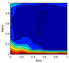
(a)

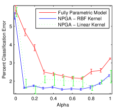
(b)

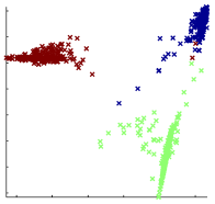
(c)

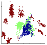
(d)

Figure 1: The effect of scaling the relative contributions of the autoencoder, logistic regressor and GP costs in the hybrid objective by modifying $\alpha$ and $\beta$. (a) Classification error on the test set on a linear scale from  6% (dark red) to  1% (dark blue) (b) Cross-sections of (a) at ${\beta\!=\!0}$ (a fully parametric model) and ${\beta\!=\!1}$ (NPGA). ($\alpha\!=\!0.5$) (c & d) Latent projections of the 1000 test cases within the latent space of the GP for a NPGA ($\alpha=0.5$) and a back-constrained GPLVM.

4.1 Oil Flow Data

As an initial empirical analysis we consider a multi-phase oil flow classification problem (Bishop and James, 1993). The data are twelve-dimensional, real-valued measurements of gamma densitometry measurements from a simulation of multi-phase oil flow. The classification task is to determine from which of three phase configurations each example originates. There are 1,000 training and 1,000 test examples. The relatively small size of these training data make them useful for empirical evaluation of different models and training procedures. We use these data primarily to address two concerns:

• To what extent does the nonparametric guidance of an unsupervised parametric autoencoder improve the learned feature representation with respect to the classification objective?

• What additional benefit is gained through using nonparametric guidance over simply incorporating a parametric mapping to the labels?

To address these questions, we construct a new objective that linearly blends our proposed supervised guidance cost $L_{\rm GP}(\phi,\boldsymbol{\Gamma})$ with the one proposed by Bengio et al. (2007), referred to as $L_{\rm LR}(\phi,\boldsymbol{\Gamma})$:

$$L(\phi,\psi,\Lambda,\boldsymbol{\Gamma}\,;\,\alpha,\beta) =(1\!-\!\alpha)L_{\rm auto}(\phi,\psi)$$

$$+\alpha((1\!-\!\beta)L_{\rm LR}(\phi,\Lambda)$$

$$+\beta L_{\rm GP}(\phi,\boldsymbol{\Gamma})),$$

where ${\beta\in[0,1]}$. $\Lambda$ are the parameters of a multi-class logistic regressor that maps to the labels. Thus, $\alpha$ controls the relative importance of supervised guidance, while $\beta$ controls the relative importance of the parametric and nonparametric supervised guidance.

A grid search over $\alpha$ and $\beta$ was performed at intervals of $0.1$ to assess the benefit of the nonparametric guidance. At each interval a model was trained for 100 iterations and classification performance was assessed via logistic regression on the hidden units of the encoder. Notice how the cost $L_{\rm LR}(\phi,\Lambda)$ is specifically tailored to this situation. The encoder used 250 noisy rectified linear (NRenLU (Nair and Hinton, 2010)) units, and zero-mean Gaussian noise with a standard deviation of 0.05 was added to the inputs of the autoencoder cost. A subset of 100 training samples was used to make the problem more challenging. Each experiment was repeated 20 times with random initializations. The GP label mapping used an RBF kernel and worked on a projected space of dimension ${H\!=\!2}$.

Results are presented in Fig. 1. Fig. 1b demonstrates that performance improves by integrating out the label map, even when compared with direct optimization under the discriminative family that will be used at test time. Figs. 1c and 1d provide a visualisation of the latent representation learned by NPGA and a standard back-constrained GPLVM. We see that the former embeds much more class-relevant structure than the latter.

An interesting observation is that a simple linear kernel also tends to outperform parametric guidance (see Fig. 1b). This doesn’t mean that any kernel will work for any problem. However, this confirms that the benefit of our approach is achieved mainly through integrating out the label mapping, rather than having a more powerful nonlinear mapping to the label.

4.2 Small NORB Image Data

As a second empirical analysis, the NPGA is evaluated on a challenging dataset with multiple discrete and real-valued labels. The small NORB data (LeCun et al., 2004) are stereo image pairs of fifty toys belonging to five generic categories. Each object was imaged under six lighting conditions, nine elevations and eighteen azimuths. The objects were divided evenly into test and training sets yielding 24,300 examples each.

The variations in the data resulting from the different imaging conditions impose significant nuisance structure that will invariably be learned by a standard autoencoder. Fortunately, these variations are known a priori. In addition to the class labels, there are two real-valued vectors (elevation and azimuth) and one discrete vector (lighting type) associated with each image. In our empirical analysis we examine two questions:

• As the autoencoder attempts to coalesce the various sources of structure into its hidden layer, can the NPGA guide the learning in such a way as to separate the class-invariant transformations of the data from the class-relevant information?

• Are the benefits of nonparametric guidance still observed in a larger scale classification problem, when mini-batch training is used?

Classes

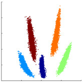
(a)

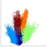
(b)

Elevation

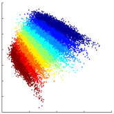
(c)

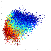
(d)

Lighting

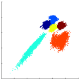
(e)

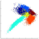
(f)

Figure 2: Visualisations of the NORB training (left) and test (right) data latent space representations in the NPGA, corresponding to class (first row), elevation (second row), and lighting (third row). Colors correspond to class labels.

Model	Accuracy
Autoencoder + 4(Log)reg ($\alpha=0.5$)	85.97%
GPLVM	88.44%
SGPLVM (4 GPs)	89.02%
NPGA (4 GPs Lin – $\alpha\!=\!0.5$)	92.09%
Autoencoder	92.75%
Autoencoder + Logreg ($\alpha=0.5$)	92.91%
NPGA (1 GP NN – $\alpha\!=\!0.5$)	93.03%
NPGA (1 GP Lin – $\alpha\!=\!0.5$)	93.12%
NPGA (4 GPs Mix – $\alpha\!=\!0.5$)	94.28%
K-Nearest Neighbors	83.4%
(LeCun et al., 2004)
Gaussian SVM	88.4%
(Salakhutdinov and Larochelle, 2010)
3 Layer DBN	91.69%
(Salakhutdinov and Larochelle, 2010)
DBM: MF-FULL	92.77%
(Salakhutdinov and Larochelle, 2010)
Third Order RBM	93.5%
(Nair and Hinton, 2009)

Table 1: Experimental results on the small NORB data test set. Relevant published results are shown for comparison. NN, Lin and Mix indicate neural network, linear and a combination of neural network and periodic covariances respectively.

To address this question, an NPGA was employed with GPs mapping to each of the four labels. Each GP was applied to a unique partition of the hidden units of an autoencoder with 2400 NReLU units. A GP mapping to the class labels was applied to half of the hidden units and operated on a ${H\!=\!4}$ dimensional latent space. The remaining 1200 units were divided evenly among GPs mapping to the three auxiliary labels. As the lighting labels are discrete, they were treated similarly to the class labels, with ${H\!=\!2}$. The elevation labels are continuous, so the GP was mapped directly to the labels, with ${H\!=\!2}$. Finally, as the azimuth is a periodic signal, a periodic kernel was used for the azimuth GP, with ${H\!=\!1}$. This elucidates a major advantage of our approach, as the GP provides flexibility that would be challenging with a parametric mapping.

This configuration was compared to an autoencoder (${\alpha\!=\!0}$), an autoencoder with parametric logistic regression guidance and a similar NPGA where only a GP to classes was applied to all the hidden units. A back-constrained GPLVM and SGPLVM were also applied to these data for comparison. The results are reported in Table 1. A visualisation of the structure learned by the GPs is shown in Figure 2.

The model with 4 GPs with nonlinear kernels obtains an accuracy of 94.28% and significantly outperforms all other models, achieving to our knowledge the best (non-convolutional) results for a shallow model on this dataset. Applying nonparametric guidance to all four of the signals appears to separate the class relevant information from the irrelevant transformations in the data. Indeed, a logistic regression classifier trained only on the 1200 hidden units on which the class GP was applied achieves a test error of 94.02%, implying that half of the latent representation can be discarded with virtually no discriminative penalty.

One interesting observation is that, for linear kernels, guidance with respect to all labels decreases the performance compared to using guidance only from the class label (from 93.03% down to 92.09%). An autoencoder with parametric guidance to all four labels was tested as well, mimicking the configuration of the NPGA, with two logistic and two gaussian outputs operating on separate partitions of the hidden units. This model achieved only 86% accuracy. These observations highlight the advantage of the GP formulation for supervised guidance, which gives the flexibility of choosing an appropriate kernel for different label mappings (e.g. a periodic kernel for the rotation label).

5 Conclusion

In this paper we observe that the back-constrained GPLVM can be interpreted as the infinite limit of a particular kind of autoencoder. This relationship enables one to learn the encoder half of an autoencoder while marginalizing over decoders. We use this theoretical connection to marginalize over functional mappings from the latent space of the autoencoder to any auxiliary label information. The resulting nonparametric guidance encourages the autoencoder to encode a latent representation that captures salient structure within the input data that is harmonious with the labels. Specifically, it enforces the requirement that a smooth mapping exists from the hidden units to the auxiliary labels, without choosing a particular parameterization. By applying the approach to two data sets, we show that the resulting nonparametrically guided autoencoder improves the latent representation of an autoencoder with respect to the discriminative task. Finally, we demonstrate on the NORB data that this model can also be used to discourage latent representations that capture statistical structure that is known to be irrelevant through guiding the autoencoder to separate the various sources of variation. This achieves state-of-the-art performance for a shallow non-convolutional model on NORB.

References

- Adams et al. (2010) R. P. Adams, Z. Ghahramani, and M. I. Jordan. Tree-structured stick breaking for hierarchical data. In Neural Information Processing Systems, 2010.
- Bengio et al. (2007) Y. Bengio, P. Lamblin, D. Popovici, and H. Larochelle. Greedy layer-wise training of deep networks. In Neural Information Processing Systems, pages 153–160, 2007.
- Bishop and James (1993) C. M. Bishop and G. D. James. Analysis of multiphase flows using dual-energy gamma densitometry and neural networks. Nuclear Instruments and Methods in Physics Research, pages 580–593, 1993.
- Cottrell et al. (1987) G. W. Cottrell, P. Munro, and D. Zipser. Learning internal representations from gray-scale images: An example of extensional programming. In Conference of the Cognitive Science Society, pages 462–473, 1987.
- Deng et al. (2010) L. Deng, M. Seltzer, D. Yu, A. Acero, A.-R. Mohamed, and G. E. Hinton. Binary coding of speech spectrograms using a deep autoencoder. In Interspeech, 2010.
- Larochelle et al. (2007) H. Larochelle, D. Erhan, A. Courville, J. Bergstra, and Y. Bengio. An empirical evaluation of deep architectures on problems with many factors of variation. In International Conference on Machine Learning, 2007.
- Lawrence (2005) N. D. Lawrence. Probabilistic non-linear principal component analysis with Gaussian process latent variable models. Journal of Machine Learning Research, 6:1783–1816, 2005.