From one- to two-dimensional solitons in the Ginzburg-Landau model of lasers with frequency selective feedback

Abstract

We use the cubic complex Ginzburg-Landau equation coupled to a dissipative linear equation as a model of lasers with an external frequency-selective feedback. It is known that the feedback can stabilize the one-dimensional (1D) self-localized mode. We aim to extend the analysis to 2D stripe-shaped and vortex solitons. The radius of the vortices increases linearly with their topological charge, $m$, therefore the flat-stripe soliton may be interpreted as the vortex with $m=\infty$, while vortex solitons can be realized as stripes bent into rings. The results for the vortex solitons are applicable to a broad class of physical systems. There is a qualitative agreement between our results and those recently reported for models with saturable nonlinearity.

I Introduction

The field of spatial pattern formation in nonlinear systems has grown significantly in the last decades (see reviews Kivshar1989 ; CrossHohenberg1993 ; Aranson2002 ; Etrich ; Buryak2002 ; Desyatnikov2005 ; LectNotesPhys2005 ; Malomed2007 ; Barcelona ). In particular, that growth was significantly contributed to by the interest in self-localized states (“solitons”) and their stability in pattern-forming systems, both conservative and dissipative ones.

The motivation of the present work is to achieve a quasi-analytical description of the formation of stable self-localized structures in spatially-extended lasers. To this end, we consider a complex Ginzburg-Landau model with the cubic nonlinearity (CGL3), for which an analytical chirped-sech localized solution is well known in the one-dimensional (1D) setting Exact1 ; Exact2 . While this solution is always unstable, it has been shown that an additional, linearly coupled, dissipative linear equation can lead to its stabilization in coupled-waveguide models, keeping the solution in the exact analytical form Atai1998 ; Sakaguchi ; Malomed2007 . Self-localized states in a wide variety of systems described by such coupled linear and nonlinear equations, in both 1D and 2D, was recently discussed in Ref. Firth2010 .

The physical system which offers a natural realization of such models is a broad-area vertical-cavity surface-emitting laser (VCSEL), coupled to an external frequency-selective feedback (FSF). This system has been a topic of interest during the last years since it can display a variety of localized structures on top of a non-lasing background Tanguy2006 ; TanguyPRL ; Tanguy2008 ; Radwell2009 ; Radwell2010 . In this system, the (complex) intra-VCSEL field features nonlinear spatiotemporal dynamics due to two-way coupling between the optical field and the inversion of the electronic population (driven by the injection current), while the feedback field obeys a linear equation which is linearly coupled to the main equation for the intra-VCSEL field. Previous studies have modeled the VCSEL-FSF using various approximations and producing a rich variety of stable and unstable localized modes, including the fundamental soliton Paulau2008 and its complex dynamics Scroggie2009 ; Paulau2009 , as well as side-mode solitons supported by an external cavity Paulau2009 , and vortex solitons Paulau2010 .

All the above-mentioned VCSEL-FSF models have been numerically investigated including, at various levels of the approximation, physically relevant features, such as the feedback delay and electron-hole dynamics and diffusion. On the other hand, the observed phenomena feature strong similarities persisting under progressive simplifications of the model, such as replacing the feedback grating with a Lorentzian filter, the adiabatic elimination the electron-hole dynamics, and adopting instantaneous, rather than delayed, feedback Paulau2010 . This observations suggest that a simpler underlying model may be introduced. In this vein, it was implied in Ref. Firth2010 that a simplification towards a simple cubic approximation for the nonlinearity, could provide such a model of the CGL3 type. It was also noted that such a cubic approximation to the VCSEL-FSF would place it in the same class of models as those previously introduced for coupled optical waveguides with active (pumped) and passive (lossy) cores in Refs. Winful ; Atai ; Atai1998 ; Sakaguchi ; Malomed2007 , and for pulsed fiber lasers – in Ref. Kutz2008 .

In this work we demonstrate that such a CGL3 system does indeed allow stable and robust fundamental solitons in 1D, and, which is the basic novel finding, fundamental and multi-charge vortex solitons in 2D. We present the bifurcation diagram for the fundamental 1D solitons in our generalized CGL3 model, and establish their stability properties. Going over into 2D, we present numerically-generated bifurcation diagrams for the fundamental and vortex solitons, establish their stability ranges, and analyze a relation to the 1D solution. To our knowledge, the existence of stable 2D solitons and vortices supported by the cubic nonlinearity in the uniform space has not been previously reported in any physical context. As concerns the stabilization of 2D dissipative solitons by means of the feedback, provided by a linearly coupled dissipative equation, this approach was first proposed, in terms of anisotropic equations of the Kuramoto-Sivashinsky type (its 2D modification), in Ref. Feng . The model was suggested by applications to the flow of viscous fluid films, rather than optics.

While our primary motivation is provided by the VCSEL-FSF, similar soliton phenomena have been found in systems such as lasers with saturable gain and absorption Vladimirov1997 ; Rosanov2005 ; RosanovPRL ; Rosanov2003 ; Fedorov2003 and with a holding beam LugiatoLefeverModel ; FirthDamia2002 ; Damia2007 ; Damia2003 , as well as in VCSEL experiments employing coupled cavities Genevet2010 and a built-in saturable absorber Elsass2010 , see also Ref. ackemann09 for a review.

The results reported in this work may have implications to both applied and fundamental studies. On the one hand, the VCSEL-soliton systems offer a strategy for the development of devices for all-optical information processing applications. On the other hand, the results constitute a new contribution to the great variety of dynamical phenomena described by CGL systems in numerous physical contexts.

The article is organized as follows. In section II we present the model previously considered for lasers with the FSF and show how it can be reduced to a CGL3 equation coupled to a linear one. In section III we consider the stability of the zero solution, which serves both as the background for self-localized modes and the source of pattern-forming instabilities. We then review the dynamics obtained from direct simulations of the CGL3 reduced model, which reproduces the spontaneous 2D-soliton formation, which was reported, in terms of the full model, in Ref. Paulau2008 , thus justifying the use of the reduction to the cubic nonlinearity. In section IV we discuss the analytical 1D solution of our CGL3 model and produce a bifurcation diagram similar to those found in more complex models Paulau2008 ; Paulau2009 ; Paulau2010 .

In section V we report the most essential new findings for 2D solitons. First, we extend the 1D analytic solution into that for the 2D stripe-soliton family and describe this family, with an intention to identify the stripe soliton as a limiting case of vortices. Then, using polar coordinates in the 2D plane, we find and characterize a family of vortex solitons, whose radius increases linearly with the topological charge. The stability of the vortex solitons is also analyzed in this section, both for the restricted class of cylindrically-symmetric perturbations and full azimuthal perturbations. While vortex solitons with high values of topological charges $m$ are always subject to the azimuthal instability (in particular, for $m\rightarrow\infty$ it goes over into the longitudinal instability of the stripe), stable vortices with $|m|\leq 3$ are found in our CGL3 model. The paper is concluded by section VI.

II The system and model

Following Ref. Paulau2010 , we start from the model for the description of VCSELs coupled to frequency-selective feedback without delay:

$$\left\{\begin{array}[]{l}\frac{\partial E}{\partial t}=-\kappa(1+i\alpha)E+\kappa(1+i\alpha)\mu\frac{E}{1+|E|^{2}}-\\ \qquad\qquad\qquad-i\Delta_{\perp}E+F-i\omega_{m}E,\\ \frac{\partial F}{\partial t}=-\lambda F+\sigma\lambda E,\end{array}\right.$$ (1)

where $\kappa$ is the cavity decay rate, $\alpha$ is the phase-amplitude coupling factor, $\mu$ is the pump current, normalized to be $1$ at the threshold in the absence of the external feedback, $\Delta_{\perp}$ is the transverse Laplacian accounting for diffraction in the paraxial approximation, $\omega_{m}$ is the detuning of the maximum of the frequency-selective feedback profile from the laser’s frequency at the threshold without the feedback, $\lambda$ stands for the width of the frequency filter, and $\sigma$ is the feedback strength in units of $\kappa$, i.e., the threshold is reduced from $\mu=1$ at $\sigma=0$ to $\mu=1-\sigma/\kappa$.

Truncating the Taylor expansion of the saturable nonlinearity at the third order, Eq. (1) is approximated by a specific form of the following CGL3 system

$$\left\{\begin{array}[]{l}\frac{\partial E}{\partial t}=g_{0}E+g_{2}|E|^{2}E+(d+iD)\Delta_{\perp}E+F,\\ \\ \frac{\partial F}{\partial t}=-\lambda F+\tilde{\sigma}E,\end{array}\right.$$ (2)

where

$$\begin{array}[]{l}g_{0}=\kappa(1+i\alpha)(\mu-1)-i\omega_{m},\\ g_{2}=-\kappa(1+i\alpha)\mu,\\ \tilde{\sigma}=\sigma\lambda,\\ D=-1,\\ d=0.\end{array}$$ (3)

Note that $\mathrm{Re}(g_{0})$ is the total linear loss (if negative) or gain (if positive), and $\mathrm{Im}(g_{0})$ plays the role of the effective frequency detuning between the laser and the filter maximum. Further, $\mathrm{Re}(g_{2})$ is the nonlinear loss (if negative) or gain (if positive), while $\mathrm{Im}(g_{2})$ represents the self-focusing or defocusing nonlinearity. In the general case, real parameters $D$ and $d$ account for transverse diffraction and diffusion of the field. In the present work we mainly consider $d=0$, which is relevant to optics models in the spatial domain Mihalache2008 ; Herve1 ; Herve2 ; Herve3 , but it may be different from zero in other physical situations – in particular, in the temporal domain Winful ; Atai ; Atai1998 ; Malomed2007 .

This approximation of the saturable nonlinearity by the cubic expansion is justified by the fact that the higher-order nonlinearity, which usually saturates the growth of the intensity in lasers without the feedback, is no longer the main saturation mechanism in the presence of external frequency-selective feedback. Above the threshold, the nonlinear term $i\mathrm{Im}(g_{2})|E|^{2}E$ induces a frequency shift that, together with the frequency-dependent feedback, introduces an effective saturation capable of limiting the field amplitude even without nonlinear losses [although $\mathrm{Re}(g_{2})$ is typically negative for lasers].

Model (2) is precisely the CGL3 equation coupled to a linear equation. For laser models, there are usually specific relations between $g_{0}$ and $g_{2}$; however, in other physical situations all parameters of model (2) may be independent, providing for the opportunity to study different behaviors of the solutions.

III Overview of the behavior of the system

Linearizing around the zero (non-lasing) solution, the evolution of perturbations $\mathbf{\delta e}=\left(\delta E,\delta F\right)$ is governed in the Fourier space by equation

$$\frac{d}{dt}\mathbf{\delta e}(k_{\perp})=\hat{M}(k_{\perp})\mathbf{\delta e(k_{\perp})},$$ (4)

where

$$\hat{M}(k_{\perp})\equiv\left(\begin{array}[]{lr}g_{0}-(d+iD)k_{\perp}^{2}&1\\ \tilde{\sigma}&-\lambda\end{array}\right).$$ (5)

The stability of the zero solution against perturbations with wavenumber $k_{\perp}$ is determined by the eigenvalues of matrix $M$. Note that, since the stability of the zero solution is independent of nonlinearities, the analysis considered here is also valid for Eqs. (1) for corresponding parameters.

In Fig. 1 we show how the marginal stability curve changes with detuning $\omega_{m}$. Taking into account the definition of $g_{0}$, for $d=0$ matrix $M$ depends on $\omega_{m}$ and $k_{\perp}$ only through the combination $\omega_{m}+Dk^{2}_{\perp}$. Since $D=-1$, increasing $\omega_{m}$ the marginal stability curve translates rigidly to larger values of $k^{2}_{\perp}$ as displayed in the figure. The mean slope of the instability balloon depends on the value of $\alpha$ as shown in Fig. 2. An interesting property, exploited in previous works, is the existence for positive $\alpha$ and for a range of negative values of $\omega_{m}$ of a region of stability for the zero solution above the off-axis emission threshold [See Fig. 1(a)]. In this region, stable self-localized modes can be found Paulau2008 ; Paulau2009 . In contrast, for $\alpha<0$ [see Fig. 2(a) corresponding to the self-defocusing case] there is no such region for any value of $\omega_{m}$. The zero solution can be stabilized, though, by a nonzero value of diffusion $d$ as illustrated by Fig. 3. Note also that both for the self-focusing and defocusing nonlinearity the zero solution can be stabilized by filtering of spatial Fourier modes in the feedback loop, which can be modeled by a wavenumber-dependent feedback strength $\tilde{\sigma}(k_{\perp})$Paulau2007 .

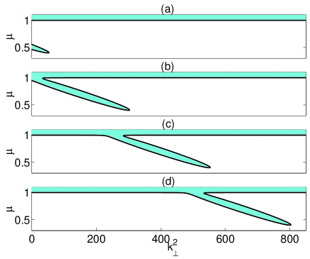
Figure 1: (Color online). Shaded are regions of the instability of the zero solution against perturbations with transverse wave number $k_{\perp}$ for different values of detuning $\omega_{m}$. The black line is the marginal-stability boundary. (a) $\omega_{m}=-250$, (b) $\omega_{m}=0$, (c) $\omega_{m}=250$, (d) $\omega_{m}=500$. Other parameters are $\sigma=60$, $\kappa=100$, $\lambda=2.71$, $\alpha=5$, $d=0$.

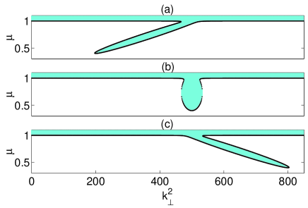
Figure 2: (Color online). The same as in Fig. 1 for different values of $\alpha$: (a) $\alpha=-5$, (b) $\alpha=0$, (c) $\alpha=5$. Other parameters are $\sigma=60$, $\kappa=100$, $\lambda=2.71$, $\omega_{m}=500$, $d=0$.

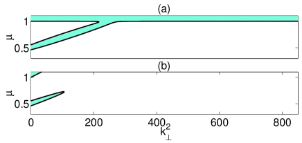
Figure 3: (Color online). The same as in Fig. 1 for different values of $d$. Even in the self-defocusing case ($\alpha<0$), the zero solution is stabilized by nonzero diffusion. Here $d=0.0$ (a) and $d=0.3$ (b). Other parameters are $\sigma=60$, $\kappa=100$, $\lambda=2.71$, $\alpha=-5$, $\omega_{m}=250$.

Different spatiotemporal regimes are possible in model (2) depending on values of the parameters. For a set of parameters close to those corresponding to Fig. 1(a), which are relevant to the dynamics of lasers, the following scenario is observed. For the pump currents in the unstable region ($\mu\approx 0.45$), small random perturbations of the zero solution grow exponentially, see Fig. 4(a), leading to a complex 2D spatiotemporal pattern, which sets in at $t\approx 80$ in Fig. 4(a). The instantaneous spatial profile of this chaotic pattern is shown in Fig. 5(a). If, starting from this regime, pump current $\mu$ is further increased up to a value at which the zero background is stable ($\mu=0.52$) [see Fig. 4(b)], a transition is observed from densely packed filaments to a 2D set of isolated quiescent solitons, see Fig. 5(b). Initially, the distance between the solitons is small, and the interaction among them leads to a partial annihilation, see the abrupt fall of the integral intensity at $t\approx 350$ in Fig. 4(a). However, when the density of solitons becomes small enough, the resulting set of quiescent cavity solitons is quasi-stationary, featuring very weak interactions.

Here we have presented the results for $\omega_{m}=-270$, for which the marginal stability curve is the same as in Fig. 1(a) but displaced 20 units to the left. For values of $\omega_{m}\approx-250$ moving solitons instead of quiescent ones are observed in the final state.

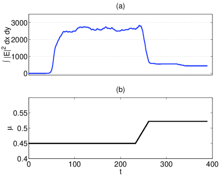
Figure 4: (Color online). (a) The total intensity of the 2D laser field, following the switch-on at the pump current $\mu=0.45$, and then the transition to a set of quiescent localized spots, achieved by ramping the pump up to $\mu=0.52$. (b) The variation of the pump current in time which gives rise to the dynamical picture displayed in panel (a). The parameters are: $\sigma=60$, $\kappa=100$, $\lambda=2.71$, $\alpha=5$, $\omega_{m}=-270$, $d=0$.

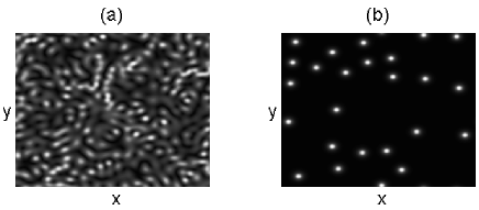
Figure 5: The instantaneous 2D amplitude profile corresponding to the regimes presented in Fig. 4, at: (a) $t=200$, corresponding to the pump current at which the zero solution is unstable and a complex spatiotemporal regime arises; (b) $t=400$, after having increased the pump current to a value for which the zero solution is stable, and the spatiotemporal pattern decays into a set of fundamental solitons.

A similar scenario is observed in one dimension, which is of special interest because exact 1D self-localized solutions are available in the CGL3 system, as we discuss below.

IV One-dimensional solitons

In the case of one transverse dimension ($\Delta_{\perp}=\partial^{2}/\partial x^{2}$) an exact analytical solution to Eqs. (2) can be found in the form of Atai1998 ; Malomed2007 ; Firth2010

$$\left\{\begin{array}[]{l}E=E_{\max}\left[\cosh(Kx)\right]^{-1-i\beta}e^{i\omega t},\\ F=F_{\max}\left[\cosh(Kx)\right]^{-1-i\beta}e^{i\omega t}.\end{array}\right.$$ (6)

Substituting expressions (6) into Eqs. (2), we eliminate

$$F_{\max}=\frac{\tilde{\sigma}}{\lambda+i\omega}E_{\mathrm{\max}},$$ (7)

and obtain the following quadratic equation for chirp $\beta$,

$$\beta^{2}+3\beta\frac{\mathrm{Re}\left[g_{2}(d-iD)\right]}{\mathrm{Im}\left[g_{2}(d-iD)\right]}-2=0,$$ (8)

which yields a single physical root, due to the condition that the field intensity

$$|E_{\mathrm{\max}}|^{2}=3\beta K^{2}\frac{d^{2}+D^{2}}{\mathrm{Im}\left[g_{2}(d-iD)\right]}$$ (9)

must be positive. Note that $\beta$ does not depend on linear coefficient $g_{0}$, but only on nonlinear coefficient $g_{2}$ and on the parameters of spatial coupling, $d$ and $D$. Once $\beta$ is known, a complex algebraic equation involving $\omega$ and $K$ is obtained. By separating the real and imaginary parts of this equation we obtain

$$K^{2}=-\frac{\mathrm{Re}(g_{0})}{\mathrm{Re}\left(\tilde{\beta}\right)}-\frac{\tilde{\sigma}\lambda}{\lambda^{2}+\omega^{2}}\frac{1}{\mathrm{Re}\left(\tilde{\beta}\right)},$$ (10)

where

$$\tilde{\beta}\equiv(1+i\beta)^{2}(d+iD).$$ (11)

Next, we obtain a cubic equation for $\omega$:

$$a_{3}\omega^{3}+a_{2}\omega^{2}+a_{1}\omega+a_{0}=0,$$ (12)

where coefficients $a_{0}$, $a_{1}$, $a_{2}$, and $a_{3}$ depend on the system’s parameters and on $\tilde{\beta}$:

$$\begin{array}[]{l}a_{3}=\mathrm{Re}(\tilde{\beta}),\\ a_{2}=\mathrm{Re}(g_{0})\mathrm{Im}(\tilde{\beta})-\mathrm{Im}(g_{0})\mathrm{Re}(\tilde{\beta}),\\ a_{1}=(\tilde{\sigma}+\lambda^{2})\mathrm{Re}(\tilde{\beta}),\\ a_{0}=a_{2}\lambda^{2}+\tilde{\sigma}\lambda\mathrm{Im}(\tilde{\beta}).\end{array}$$ (17)

Equation (12) can be solved analytically, but it is more practically relevant to solve it numerically, as in Ref. Firth2010 . To summarize, the analytical solutions can be constructed according to the following scheme.

• (i) Solve Eq. (8) for $\beta$, and choose the proper root to satisfy the positivity of $|E_{max}|^{2}$ as per Eq. (9).

• (ii) Solve Eq. (12) for $\omega$ with the coefficients defined by Eqs. (11, 17), and $\beta$ produced by the previous step.

• (iii) Calculate $K$ using Eqs. (10, 11), and $\omega$, with $\beta$ produced by two previous steps.

• (iv) Calculate $E_{max}$ using Eq. (9).

• (v) Calculate $F_{max}$ using Eq. (7).

Once all parameters of solution (6) are determined, the stability of this solution can be analyzed following the numerical procedure developed in Ref. Paulau2010 .

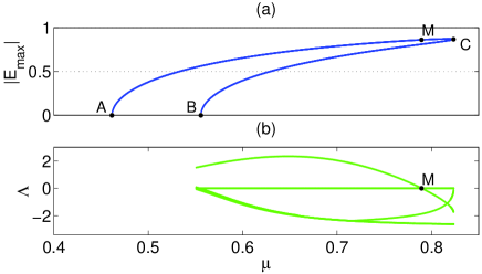
Figure 6: (Color online). The bifurcation diagram for analytical solution (6). (a) The amplitude (absolute value of the field at the center of the fundamental soliton) as a function of the pump current. (b) The growth rate of unstable, neutral and least-damped stable perturbation eigenmodes versus the pump current $\mu$. Point $M$ designates the drift instability of the soliton. The parameters are $\omega_{m}=-250$, $\alpha=5$, $\kappa=100$, $\sigma=60$, $\lambda=2.71$.

Fig. 6(a) shows the bifurcation diagram for the localized quiescent solitons (6), using parameter values typical for the lasers models. Point A corresponds to the pump threshold for on-axis emission. For the pump levels $\mu$ between points A and B the zero background is unstable as shown in Fig. 1(a). These points coincide with the origin of two branches of localized structures. The two branches collide at C and disappear through a saddle-node bifurcation.

Figure 6(b) shows the real part of the most relevant eigenvalues resulting of the stability analysis of the upper branch [the one connecting points C, M and A in Fig. 6(a)]. The soliton solution is stable between points C and M, and a drift instability appears at point M Paulau2009 . The instability spectrum is not shown between points A and B because the background zero solution is unstable. The lower branch of soliton solution connecting points B and C in Fig. 6(a) is entirely unstable, as usual Winful ; Atai .

Direct simulations starting from the 1D analytic soliton in the unstable region (to the left of point M in Fig. 6) shows the development of the drift instability, see Fig. 7. Notice that once the drift instability sets in the soliton moves away from its original location at a constant speed.

The overall scenario is very similar to that found in previous numerical works for the saturable nonlinearity Paulau2008 ; Paulau2009 ; Paulau2010 , suggesting that the present CGL3 system indeed represents a simple underlying model which captures the essential features of more realistic, but also more involved, models.

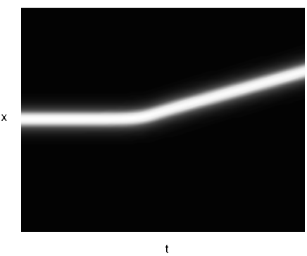
Figure 7: Spatiotemporal dynamics of the 1D soliton in the course of the development of the drifting instability. The parameters are as in Fig. 6, for $\mu=0.7$.

V Two-dimensional self-localized solutions: stripes, fundamental, and vortex solitons

In 2D ($\Delta_{\perp}=\frac{\partial^{2}}{\partial x^{2}}+\frac{\partial^{2}}{\partial y^{2}}$), the 1D solution (6) can be generalized to a continuous family of the stripe-soliton solutions, parameterized by transverse wavenumber $k_{y}$:

$$\left\{\begin{array}[]{l}E=E_{\max}\left[\cosh(Kx)\right]^{-1-i\beta}e^{i\omega t}e^{ik_{y}y},\\ F=F_{\max}\left[\cosh(Kx)\right]^{-1-i\beta}e^{i\omega t}e^{ik_{y}y}.\end{array}\right.$$ (18)

The only difference from the above 1D solution is a modification of linear coefficient $g_{0}$, which is replaced by $\tilde{g}_{0}=g_{0}-(d+iD)k_{y}^{2}$. This solution is shown in Fig. 8(a,b). We have found the whole family of the stripe solitons as a function of $k_{y}$, see Fig. 9. They exist only for values of $k_{y}^{2}$ below a certain value beyond which the frequency shift introduced by $k_{y}$ pushes the solution outside the frequency range of the feedback filter. The solution with largest amplitude, marked by a filled circle, corresponds to $k_{y}$ such that $\omega=0$. Fig. 9(c), shows the largest real parts of the eigenvalues obtained from the linear stability analysis in the $x$-direction. The stripe-soliton undergoes a drift instability similar to the one of the 1D soliton described in the previous section. Here the stripe as a whole would start to move either to the left or to the right of its axis. Interestingly enough the drift instability takes place at a value of $k_{y}=k_{y}^{c}$ which, within the numerical accuracy, coincides with the value for which the solution has $\omega=0$. The critical value $k_{y}^{c}$ will be very relevant later when studying the radial dynamics of vortices. In any case, 2D stripe-solitons are always unstable to perturbations in the $y$-direction, breaking up into a number of fundamental (spot) solitons.

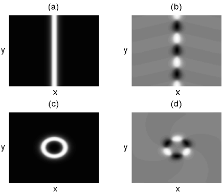
Figure 8: The spatial profile of the amplitude (a) and real part of the field (b) for the unstable 2D stripe soliton (18). (c) and (d): The same as (a) and (b) for a stable vortex with $m=3$. Here $\mu=0.52$ and other parameters are the same as in Fig. 4.

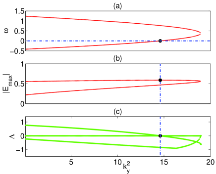
Figure 9: (Color online). The continuous family of 2D stripe solitons parameterized by $k_{y}$, for $\mu=0.52$ and other parameters taken as in Fig. 4. (a) Frequency $\omega$, (b) the soliton’s amplitude $|E_{\max}|$, and (c) growth rates of the unstable neutral and least damped stable eigenmodes (the stability is considered against perturbations depending only on the $x$ coordinate).

We now proceed to fully localized 2D solutions. There are two types of stable 2D modes: fundamental solitons with the bell-like intensity profile, see Fig. 5(b), and ring-shaped vortex solitons, see Fig. 8(c). Vortex solitons with integer topological charge $m$ can be looked for as $E(r,\phi)=E_{0}(r)e^{im\phi}$, where $(r,\phi)$ are polar coordinates with the origin at the pivot of the vortex Montagne1997 ; CrasovanMalomedMihalache2000 ; Mihalache2008 ; Desyatnikov2000 ; Towers2001 ; Herve3 . The fundamental 2D soliton corresponds to $m=0$, with the maximum at the origin. Every $m$ vortex has a mirror-image $-m$ vortex, therefore for the sake of simplicity in what follows we will consider vortex solitons with $m>0$.

Figure 8 shows the similarity between a vortex mode and the stripe soliton. Roughly speaking, the vortex may be considered as a stripe bent into a closed circle, at least for large values of $m$. Following this similarity, we study the radial dynamics of vortices using the radial version of Eq. (2), with

$$\Delta_{\perp}=\frac{\partial^{2}}{\partial r^{2}}+\frac{1}{r}\frac{\partial}{\partial r}-\frac{m^{2}}{r^{2}}.$$ (19)

Using 1D analytical solution (6) to define the initial condition as $E_{\mathrm{ini}}(r)=E_{0}(r=R_{0}+x)$, we simulated Eq. (2) with the Laplacian taken as per Eq. (19), with fixed $m$. If the initial ring radius $R_{0}$ is too small, the field decays to zero, but for $R_{0}$ large enough we observed the evolution of radius $r_{\max}$ corresponding to the maximum field amplitude towards equilibrium radius $R^{\mathrm{st}}(m)$ of the vortex soliton of charge $m$, see Fig. 10. If $R_{0}$ is much larger than $R^{\mathrm{st}}(m)$, we observed that the vortex shrank at a constant speed, which was followed by relaxation oscillations as $R^{\mathrm{st}}(m)$ was approached. Actually, this is an unusual behavior, very different from the typical curvature-driven dynamics Denmark ; Gomila01 . The constant shrinkage speed may be explained by considering the quasi-1D dynamics of the stripe-soliton solution. If the initial condition has a very large $r_{\max}$, the ring can be considered locally as a stripe-soliton with $k_{y}\approx 0$, which is drift-unstable (see Fig. 9). The overall curvature of the ring breaks the left-right symmetry the stripe had in the direction perpendicular to the axis. The symmetry breaking is such that the drift takes place towards the center and hence the ring as a whole starts contracting at a constant speed. The first stage of the dynamics shown in Fig. 10 (at $t<7$) is, thus, essentially the same as in Fig. 7. As radius $r_{\max}$ shrinks, the effective wavenumber $k_{y}$ increases, eventually suppressing the drift instability and the ring relaxes to the stable radius $R^{\mathrm{st}}(m)$.

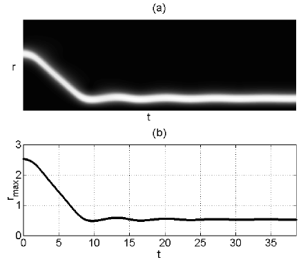
Figure 10: (a) The spatiotemporal dynamics of the radial profile of the field amplitude relaxing towards the equilibrium radius of the vortex with $m=2$. Here $\mu=0.52$ and other parameters are as in Fig. 4. (b) The dynamics of position $r_{\max}$ of the maximum of the field.

Running the simulations for different (large enough) values of $m$, we have produced the dependence of the equilibrium radius $R^{\mathrm{st}}$ on the topological charge $m$, which turns out to be linear, see Fig. 11. Therefore, vortex rings expand as $m$ increases, tending towards the stripe solution in the limit of $m\rightarrow\infty$. The inverse of the slope of the line in Fig. 11, $R^{\mathrm{st}}(m)/m$, is the transverse circular wavenumber $k_{c}$, which is, evidently, nearly constant for all vortices. The value of $k_{c}$ turns out be very similar to the drift-instability critical wavenumber of the soliton stripe, $k_{y}^{c}$ considered above.

The mechanism leading to 2D stable vortices discussed here has no counterpart in simple curvature driven dynamics of fronts connecting two equivalent states Denmark ; Gomila01 . In these systems, 1D fronts in a 2D system may be subject to modulational instabilities but not to drift ones. Therefore there is no transient regime in which the ring radius changes at a constant rate. The existence of the 1D soliton drift instability plays a critical role in the dynamics of 2D solitons and determines its stationary size.

The radial equation allows one to study the radial dynamics independently of the presence of azimuthal instabilities. In fact, as in the case of the stripe soliton, vortices with large $m$ are azimuthally unstable in the full 2D problem. The curvature can, however, prevent the azimuthal instability for small topological charges, and vortices may be stable up to a certain value of $m$ CrasovanMalomedMihalache2000 ; Paulau2010 . Figure 8(c,d) shows, for instance, a stable vortex for $m=3$.

Finally, following the method described in Ref. Paulau2010 , we have computed the bifurcation diagrams of the solitons with $m=0,1$ and analyzed their stability, see Fig. 12. The fundamental soliton (vortex) is stable between points $M_{0}$ and $C_{0}$ ($M_{1}$ and $C_{1}$). Point $M_{0}(M_{1})$ again corresponds to the onset of the drifting instability of the state as a whole. The branches connecting points $B$ and $C_{0}$ ($B$ and $C_{1}$) correspond to the solitons which play the role of the unstable separatrix. The fundamental 2D soliton and the $m=1$ vortex have quite a similar bifurcation diagram. As compared to 1D solitons, see Fig. 6, points A and B correspond to the limits of the region where the background zero solution is unstable to homogeneous perturbations and therefore are the same, however here points C and M are located at a lower pump value.

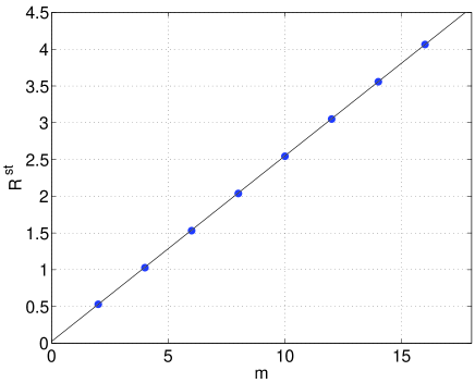
Figure 11: (Color online). The equilibrium radius $R^{\mathrm{st}}$ of the vortex solitons versus the topological charge. Parameters are as in Fig. 10. Filled circles mark even integer values of $m$, while the solid line is a linear fitting. Figure 10 corresponds to the leftmost point in this figure.

In addition, we have observed stable vortices with $m=2$ and $3$. The region of their existence is almost identical to the existence region of $m=1$ vortex, while the stability region is narrower and lies inside M₁C₁ interval of Fig. 12.

In the case of saturable nonlinearity, system (1) gives also rise to fundamental 2D solitons and vortices as encountered here Paulau2010 . The region of existence and the bifurcation diagrams are quite similar to the ones shown here. This is a clear indication that the present CGL3 model is indeed relevant for other systems, for which the analysis in terms of exact stripe solutions is not possible.

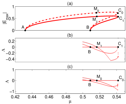
Figure 12: (Color online). (a) The amplitude of the soliton with $m=0$ (dash-dotted line) and $m=1$ (solid line) versus the pump current. (b) The growth rate of the 6 localized modes with highest $\Lambda$, including unstable, neutral and least damped stable eigenmodes for the solution branch C₁M₁A in panel (a). (c) The same as (b) but for the solution branch C₀M₀A in panel (a). Parameters are the same as used above in this section.

VI Summary

In this work, we have introduced the system of coupled cubic complex Ginzburg-Landau equation and additional dissipative linear equation as the model of laser cavities with the external frequency-selective feedback. We have observed a qualitative agreement with the results recently obtained in models with the saturable nonlinearity Paulau2008 ; Paulau2009 ; Paulau2010 . In particular, the stability of the fundamental 2D solitons is obvious in the case of the saturable nonlinearity, while it is a nontrivial finding in the cubic model. Using analytical considerations and numerical analysis, we have shown that 2D vortex solitons can be interpreted as stripe solitons bent into rings (as illustrated by Fig. 8). This correspondence is clear for $m\rightarrow\infty$, but it actually holds too for rather small $m$, since the circular transverse wavenumber appears to be the same for all $m$ (see Fig. 11). In such a way, we have established the connection between 1D and 2D solitons.

In our system of the coupled cubic and linear equations, we have found stable 1D and 2D solitons, including vortices. These results are important, as they show that this system may be considered as the fundamental model underlying a wide class of stable soliton lasers. The simplicity and flexibility of the linear coupling has previously been shown to provide the existence of stable 1D solitons in the models of dual-core waveguides Winful ; Atai ; Atai1998 ; Sakaguchi ; Malomed2007 . Our extension of this approach into the spatial domain, and into 2D, means that models of this class may be useful to describe and analyze stable self-localization for a wide variety of physical systems.

We acknowledge financial support from MICINN (Spain) and FEDER (EU) through Grant No. FIS2007-60327 FISICOS.

References

- (1) Y. S. Kivshar and B. A. Malomed, Rev. Mod. Phys. 61, 763 (1989).
- (2) M. C. Cross and P. C. Hohenberg, Rev. Mod. Phys. 65, 851 (1993).
- (3) I. S. Aranson and L. Kramer, Rev. Mod. Phys. 74, 99 (2002).
- (4) C. Etrich, F. Lederer, B. A. Malomed, T. Peschel, and U. Peschel, Progress in Optics, ed. E. Wolf, 41, 483 (2000).
- (5) A. V. Buryak, P. D. Trapani, D. V. Skryabin, and S. Trillo, Phys. Rep. 370, 63 (2002).
- (6) A. S. Desyatnikov, Y. S. Kivshar, and L. Torner, Progress in Optics, ed. E. Wolf, 47, 291 (2005).
- (7) “Dissipative solitons,” Lect. Notes Phys. 661, edited by N. Akhmediev and A. Ankiewicz, (Springer, New York 2005).
- (8) B. A. Malomed, Chaos 17, 037117 (2007).
- (9) Y. V. Kartashov, B. A. Malomed, and L. Torner, Solitons in nonlinear lattices, Rev. Mod. Phys., in press.
- (10) L. M. Hocking and K. Stewartson, Proc. R. Soc. London, Ser. A 326, 289 (1972).
- (11) N. R. Pereira and L. Stenflo, Phys. Fluids 20, 1733 (1977).
- (12) J. Atai and B. A. Malomed, Phys. Lett. A 246, 412 (1998).
- (13) H. Sakaguchi and B. A. Malomed, Physica D 147, 273 (2000).
- (14) W. J. Firth and P. V. Paulau, Eur. Phys. J. D 59, 13 (2010).
- (15) Y. Tanguy, T. Ackemann and R. Jäger, Phys. Rev. A 74, 053824 (2006).
- (16) Y. Tanguy, T. Ackemann, W. J. Firth and R. Jäger, Phys. Rev. Lett. 100, 013907 (2008).
- (17) Y. Tanguy, N. Radwell, T. Ackemann, and R. Jäger, Phys. Rev. A 78, 023810 (2008).
- (18) N. Radwell and T. Ackemann, IEEE J. Quantum Electron. 45, 1388 (2009).
- (19) N. Radwell, C. McIntyre, A. Scroggie, G.-L. Oppo, W. J. Firth, and T. Ackemann, Eur. Phys. J. D 59, 121 (2010).
- (20) P. V. Paulau, D. Gomila, T. Ackemann, N. A. Loiko, and W. J. Firth, Phys. Rev. E 78, 016212 (2008).
- (21) A. J. Scroggie, W. J. Firth and, G.-L. Oppo, Phys. Rev. A 80, 013829 (2009).
- (22) P. V. Paulau, D. Gomila, P. Colet, M. A. Matias, N. A. Loiko, and W. J. Firth, Phys. Rev. A 80, 023808 (2009).
- (23) P. V. Paulau, D. Gomila, P. Colet, N. A. Loiko, N. N. Rosanov, T. Ackemann and W. J. Firth, Opt. Exp. 18, 8859 (2010).
- (24) B. A. Malomed and H. G. Winful, Phys. Rev. E 53, 5365 (1996).
- (25) J. Atai and B. A. Malomed, Phys. Rev. E 54, 4371 (1996).
- (26) J. N. Kutz and B. Sandstede, Opt. Exp. 16, 636 (2008).
- (27) B. F. Feng, B. A. Malomed, and T. Kawahara, Phys. Rev. E 66, 056311 (2002).
- (28) A. G. Vladimirov, N. N. Rosanov, S. V. Fedorov, and G. V. Khodova, Quantum Electronics 27, 949-952 (1997).
- (29) N. N. Rosanov, S. V. Fedorov, and A. N. Shatsev, Appl. Phys. B 81, 937 (2005).
- (30) N. N. Rosanov, S. V. Fedorov, and A. N. Shatsev, Phys. Rev. Lett. 95, 053903 (2005).
- (31) N. N. Rosanov, S. V. Fedorov, and A. N. Shatsev, Optics and Spectroscopy 95, 902 (2003).
- (32) S. V. Fedorov, N. N. Rosanov, and A. N. Shatsev, N. A. Veretenov, and A. G. Vladimirov, IEEE Journal of Quantum Electronics 39, 197 (2003).
- (33) L. A. Lugiato and R. Lefever, Phys. Rev. Lett. 58, 2209 (1987).
- (34) W. J. Firth, G. K. Harkness, A. Lord, J. M. McSloy, D. Gomila, and P. Colet, J. Opt. Soc. Am. B 19, 747 (2002).
- (35) D. Gomila, A. J. Scroggie, and W. J. Firth, Physica D 227, 70 (2007).
- (36) D. Gomila and P. Colet, Phys. Rev. A 68, 011801(R) (2003).
- (37) P. Genevet, S. Barland, M. Giudici, and J. R. Tredicce, Phys. Rev. Lett. 104, 223902 (2010).
- (38) T. Elsass, K. Gauthron, G. Beaudoin, I. Sagnes, R. Kuszelewicz and S. Barbay, Eur. Phys. J. D 59, 91 (2010).
- (39) T. Ackemann, W. J. Firth and G.-L. Oppo, Adv. in Atomic, Molecular, and Optical Physics 57, 323 (2009).
- (40) D. Mihalache, D. Mazilu, F. Lederer, H. Leblond, and B. A. Malomed, Phys. Rev. A 77, 033817 (2008).
- (41) H. Leblond, B. A. Malomed, and D. Mihalache, Phys. Rev. A 80, 033835 (2009).
- (42) D. Mihalache, D. Mazilu, V. Skarka, B. A. Malomed, H. Leblond, N. B. Aleksić, and F. Lederer, Phys. Rev. A 82, 023813 (2010).
- (43) V. Skarka, N. B. Aleksić, H. Leblond, B. A. Malomed, and D. Mihalache, Phys. Rev. Lett. 105, 213901 (2010).
- (44) P. V. Paulau, A. J. Scroggie, A. Naumenko, T. Ackemann, N. A. Loiko, and W. J. Firth, Phys. Rev. E 75, 056208 (2007).
- (45) R. Montagne, E. Hernández-García, A. Amengual and M. San Miguel, Phys. Rev. E 56, 151 (1997).
- (46) L.-C. Crasovan, B. A. Malomed, and D. Mihalache, Phys. Rev. E 63, 016605 (2000).
- (47) A. Desyatnikov, A. Maimistov, and B. Malomed, Phys. Rev. E 61, 3107 (2000).
- (48) I. Towers, A. V. Buryak, R. A. Sammut, B. Malomed, L.-C. Crasovan, and D. Mihalache, Phys. Lett. A 288, 292 (2001).
- (49) P. L. Christiansen, N. Grønbech-Jensen, P. S. Lomdahl, and B. A. Malomed, Physica Scripta 55, 131 (1997).
- (50) D. Gomila, P. Colet, G.-L. Oppo, and M. San Miguel, Phys. Rev. Lett. 87, 194101 (2001).