Accurate Mass Estimators for NFW Halos

Abstract

We consider the problem of estimating the virial mass of a dark halo from the positions and velocities of a tracer population. Although a number of general tools are available, more progress can be made if we are able to specify the functional form of the halo potential (although not its normalization). Here, we consider the Navarro-Frenk-White (NFW) halo and develop two simple estimators. We demonstrate their effectiveness against numerical simulations and use them to provide new mass estimates of Carina, Fornax, Sculptor, and Sextans dSphs.

1 Introduction

There are many instances when we wish to estimate the mass of a dark halo based on properties of a tracer population. This includes calculating the masses, of the Milky Way and M31 halos from the positions and velocities of satellite galaxies, globular clusters and halo stars; of the dark halos of dwarf spheroidal galaxies from the projected positions and velocities of constituent stars; of galaxy clusters from the motions of member galaxies.

There has been much previous work on this problem. Early estimators were based on the virial theorem, but Bahcall & Tremaine (1981) showed that such estimators are inefficient, biased and, inconsistent, and replaced them with the projected mass estimator. Their original estimator was tailored for test particles around a point mass whereas Heisler et al. (1985) extended it for self-consistent cases. This was modified by Watkins et al. (2010) to deal with tracer populations whose number density does not necessarily trace an extended underlying dark matter distribution. An & Evans (2011) on the other hand devised a general theory of mass estimators under the assumption that the dark matter density law is known, although the normalization is not.

Here, we start by accepting that numerous studies have shown us that the dark halos have the universal form, namely (Navarro et al., 1995, henceforth NFW),

$$\rho(r)\propto\frac{1}{r\,(a+r)^{2}}$$ (1)

where $a$ is the scale radius. We wish to find the virial mass $M_{\mathrm{vir}}$, which is the mass within the virial radius $r_{\mathrm{vir}}$. We deduce the enclosed mass $M(r)$ within the radius $r$;

$$M(r)\propto\mu\biggl{(}\frac{r}{a}\biggr{)}\,;\qquad\mu(x)\equiv\log(1+x)-\frac{x}{1+x}$$ (2)

and the normalized mass profile $\tilde{M}(r)$ follows as

$$\tilde{M}(r)\equiv\frac{M(r)}{M_{\mathrm{out}}}=\frac{\mu(\tilde{r})}{\mu(c)}\qquad\text{($0\leq r\leq r_{\mathrm{out}}=r_{\mathrm{vir}}$)}.$$ (3)

Here $M_{\mathrm{out}}=M(r_{\mathrm{out}})$, and $r_{\mathrm{out}}$ is the outermost data point in our sample while $\tilde{r}=r/a=cr/r_{\mathrm{vir}}$, and $c=r_{\mathrm{vir}}/a$ is the concentration parameter. We have here assumed $r_{\mathrm{out}}=r_{\mathrm{vir}}$ and so $M_{\mathrm{out}}=M_{\mathrm{vir}}$, which is the case for halo mass estimation using satellite galaxies.

The problem therefore is: Given an assumed NFW profile together with the positions and velocities of tracers that extend out to the virial radius, how can we estimate the virial mass? The aim of this Letter is to provide a ready-to-use specifically-optimized estimator for the most popular halo model with tests and applications, without burdening the reader with a plethora of mathematical derivations.

2 Two Estimators

An & Evans (2011) show that if we are willing to assume the functional form of the halo mass profile $\tilde{M}(r)$ within the given spherical region of interest, then the total dark halo mass $M_{\mathrm{vir}}$ in the same region can be estimated through a weighted average of kinematic properties of the tracers, adjusted by the boundary term. The boundary term is related to the external pressure support of the tracer population, but it is usually taken as small compared to other uncertainties and so neglected. The mass of the NFW halo is formally infinite. This means that the profile needs to be truncated at some radius, which is usually taken to be either $r_{\mathrm{out}}$ or $r_{\mathrm{vir}}$. In this paper, we suppose that the tracers are well-populated out to the virial radius so that $r_{\mathrm{out}}=r_{\mathrm{vir}}$.

We consider two cases. First, as for the Milky Way satellites, 3-d distances $r$ to and radial velocities $v_{r}$ with respect to the halo center are available for tracers. Strictly speaking, the radial velocity is with respect to the Sun, but for most practical proposes, this is almost equivalent to the the radial velocity with respect to the Galactic Center for distant tracers. Second, as for populations in most external galaxies, projected distances $R$ and line-of-sight velocities $v_{\ell}$ are available for tracers. We consider these two in turn.

2.1 True Distances and Radial Velocities

The general principle underlying all estimators is that the mass is a weighted average of the positions and velocities of the tracers. For a given choice of functional form for the dark matter potential, An & Evans (2011) showed that there is an optimum weight function. For the case of this NFW halo, this gives

$$GM_{\mathrm{vir}}=\biggl{\langle}\frac{rw(r)}{\tilde{M}(r)}v_{r}^{2}\biggr{\rangle}-\bcancel{\frac{4\pi r_{\mathrm{vir}}^{4}}{N}\nu\sigma_{r}^{2}|_{r=r_{\mathrm{vir}}}},$$ (4)

where

$$w(r)=4-2\beta(r)-\frac{1}{\mu(r/a)}\biggl{(}\frac{r}{a+r}\biggr{)}^{2}.$$ (5)

Here, $\beta$ is the Binney anisotropy parameter for the spherical system. Deason et al. (2011) analyzed properties of velocity distributions of satellites galaxies in numerical simulations of dark halos and found that typically $\beta\approx 0$. We retain $\beta$ in our formulae, but in applications we assume $\beta=0$. The last term in equation (4) is the boundary condition, which is discarded here. This gives the estimator as

$$\frac{M_{\mathrm{vir}}}{\mu(c)}\simeq\frac{1}{GN}\sum_{i=1}^{N}\frac{w(r_{i})}{\mu(r_{i}/a)}\,r_{i}v_{r,i}^{2}$$ (6)

where the index $i$ runs over the $N$ tracers. We refer to this as the NFW Mass Estimator (NFWME).

It is useful to compare this with a special case of the estimator derived by Watkins et al. (2010). They studied dark halos with density profiles that are scale-free out to the virial radius

$$\tilde{M}(r)=\biggl{(}\frac{r}{r_{\mathrm{vir}}}\biggr{)}^{1-\alpha}.$$ (7)

For this case, the weight function is a power-law, and the mass estimator becomes

$$M_{\mathrm{vir}}=\frac{(\alpha+\gamma-2\beta)\,r_{\mathrm{vir}}^{1-\alpha}}{G}\left\langle r^{\alpha}v_{r}^{2}\right\rangle$$ (8)

where $\gamma$ is the power-law index for the tracer density ($\propto r^{-\gamma}$). An & Evans (2011) have shown that the choice $\gamma=3$ corresponds to neglecting the boundary term. By contrast, Watkins et al. (2010) circumvented the effect of the boundary term by explicitly solving for the power-law solution for the tracers. Here, we recommend the choice $\gamma\approx 2.5$ for satellite galaxy populations, but $\gamma\approx 3$ for stellar populations in dark haloes. Simulations typically find that the number density of satellite galaxies falls off more slowly than the stars (e.g., Deason et al., 2011). In addition, Watkins et al. (2010) also argued that $\alpha\approx 0.5$ is a good approximation to the NFW halo, at least for the range of virial masses and concentrations appropriate to large galaxies like the Milky Way. With these particular indices, the mass estimator is in the form:

$$M_{\mathrm{vir}}\approx\frac{r_{\mathrm{vir}}^{0.5}\,(0.5+\gamma-2\beta)}{GN}\sum_{i=1}^{N}r_{i}^{0.5}v_{r,i}^{2}.$$ (9)

We refer to this as the Scale-Free Mass Estimator (SFME). Equations (6) and (9) are the fundamental results of this subsection. They provide simple formulae for the mass in terms of weighted sums of the positions and velocities. We shall test these formulae against simulations shortly.

2.2 Projected Distances and Line-of-Sight Velocities

In many situations, the radial velocities and true positions of the tracers with respect to the center of the halo are not direct observables, but the line-of-sight velocities and projected positions are. The adjustment of the estimator for this happenstance is covered in An & Evans (2011, Sect. 4).

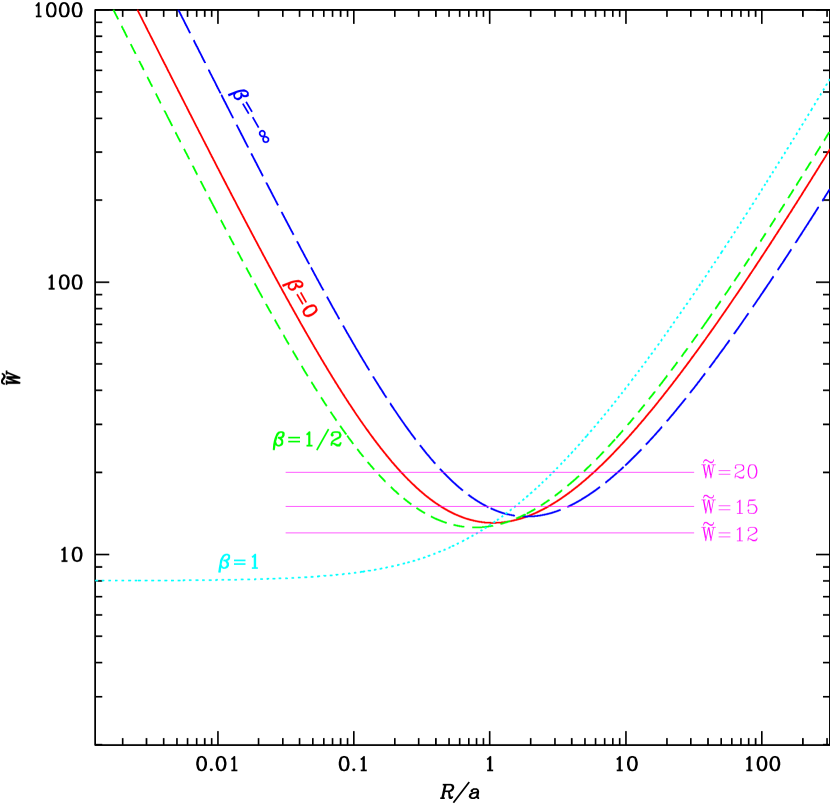
Figure 1: The invariant normalized weight function $\tilde{W}(\tilde{R})$ for the NFW profile as a function of the normalized projected separation $\tilde{R}=R/a$. The weight function can be series-expanded at $\tilde{R}=0$ with its leading term behaving as $\sim\tilde{R}^{-1}$ unless $\beta=1$. On the other hand, asymptotically toward $\tilde{R}\rightarrow\infty$, we find that $\tilde{W}(\tilde{R})\sim\tilde{R}/\log\tilde{R}$.

Here, we would like to find the weight function $W(R)$ of $R$ such that $\langle v_{\ell}^{2}W(R)\rangle=\langle rw(r)\tilde{M}^{-1}v_{r}^{2}\rangle$, which is to be substituted into the mass estimator. An & Evans (2011) show that this leads to an integral equation and the weight function $W(R)$ can be computed, at least numerically. The invariant (i.e., independent of $c$) normalized weight functions $\tilde{W}(\tilde{R})\equiv W(R)/[a\mu(c)]$ for the NFW profile for some constant $\beta$ are shown in Figure 1.

Notice that for much of the range occupied by the tracers and of the physical range of the anisotropy parameter ($1/2>\beta>-1$ or the axis ratio of the velocity ellipsoid no more extreme than $1:\sqrt{2}$), the weight function in Figure 1 is constant to a good approximation, $\tilde{W}(\tilde{R})\approx 15$, so that

$$\frac{M_{\mathrm{vir}}}{\mu(c)}\simeq\frac{a}{GN}\sum_{i=1}^{N}\tilde{W}\Bigl{(}\frac{R_{i}}{a}\Bigr{)}\,v_{\ell,i}^{2}\approx\frac{15a}{GN}\sum_{i=1}^{N}v_{\ell,i}^{2}.$$ (10)

Interestingly, this indicates that $M(a)\approx 3G^{-1}a\langle v_{\ell}^{2}\rangle$ since $M_{\mathrm{vir}}/\mu(c)=M(r)/\mu(r/a)$ and $\mu(1)\approx 0.2$. In what follows, we however use the numerically obtained weight function for the mass estimator, which is the projected analog of equation (6).

We will again compare this estimator to the projected analog of the scale-free estimator. If $\beta$ is a finite constant and the mass profile is in the scale-free form in equation (7), we find that (c.f., Watkins et al., 2010, eqs. 26 & 27)

$$M_{\mathrm{vir}}=\frac{4\Gamma\bigl{(}\frac{\alpha+5}{2}\bigr{)}}{\sqrt{\pi}\Gamma\bigl{(}\frac{\alpha}{2}+1\bigr{)}}\frac{(\alpha+\gamma-2\beta)\,r_{\mathrm{vir}}^{1-\alpha}}{\alpha+3-(\alpha+2)\beta}\frac{\left\langle R^{\alpha}v_{\ell}^{2}\right\rangle}{G}.$$ (11)

Specializing to the case $\alpha\approx 0.5$ and $\gamma\approx 3$, we find

$$M_{\mathrm{vir}}\approx\frac{4r_{\mathrm{vir}}^{0.5}}{GN}\,\biggl{(}\frac{1-\frac{4}{7}\beta}{1-\frac{5}{7}\beta}\biggr{)}\ \sum_{i=1}^{N}R_{i}^{0.5}v_{\ell,i}^{2}.$$ (12)

This is the projected analog of equation (9). Equations (10) and (12) are the fundamental results of this subsection.

3 Applications

3.1 Numerical Simulations

We begin by testing our estimators against simulations. The Galaxies-Intergalactic Medium Interaction Calculation (GIMIC) suite of simulations is described in detail in Crain et al. (2009). It consists of a set of hydrodynamical resimulations of five nearly spherical regions ($\sim 20h^{-1}\ \mbox{Mpc}$ in radius) extracted from the Millennium Simulation (Springel et al., 2005). Deason et al. (2011) extracted from the GIMIC simulations a set of galaxies that resemble the Milky Way. The sample consists of 431 parent halos and 4,864 associated satellite galaxies.

There are a number of ways in which mock catalogs from simulations differ from the assumptions used to derive the estimators. For example, dark halos are not generally spherical, infall continues to the present day, and the observed satellites are not necessarily virialized and well-described by an equilibrium distribution. Also, notions of a constant anisotropy are probably idealized, and in practice the anisotropy will vary with radius. These systematic errors are larger than random errors on the measurements of velocities and positions.

The mass estimators provide an estimate for the total mass within the radius of the farthest tracer ($\approx r_{\mathrm{out}}$). We compute the ‘true’ mass within $r_{\mathrm{out}}\approx r_{\mathrm{vir}}$ for each halo and compare to masses found via our estimators. We use all satellites, but check that our results are not significantly affected when only luminous satellites are included. Results are obtained for the two estimators in this paper – the NFWME and the SFME – and also the virial mass estimator (VME) and the projected mass estimator (PME) of Bahcall & Tremaine (1981). The left panel of Figure 2 refers to data sets of radial velocities and true distances, and the right panel to line-of-sight velocities and projected distances. We quantify the goodness of any estimator by means of two statistical measures. First, we define the Fraction of Reasonable Estimates (FRE) as the fraction of estimates within the factor of two of the true mass (see also Deason et al., 2011). We also give the Inter Quartile Range (IQR) of the mass estimates, which gives a good indication of the spread. In all cases, we see that the NFWME and the SFME outperform the VME and PME. Interestingly, the performance of the NFWME is comparable to SFME. Given this, we recommend the use of equations (9) and (12) for practical applications.

3.2 Dwarf Spheroidal Masses

We now turn to an astrophysical problem. The recent years have seen programs to garner the radial velocities of giant stars in the nearby dwarf spheroidal galaxies (dSphs). For the brighter of the dSphs, radial velocity surveys have provided data sets of projected positions and line-of-sight velocities for thousands of stars (see e.g., Kleyna et al., 2002; Wilkinson et al., 2004; Walker et al., 2009a). This has driven new theoretical ideas, such as the claim by Strigari et al. (2008) that all the dSphs shared a common mass scale of $\sim 10^{7}\ \mbox{M${}_{\sun}$}$ within 300 pc. The data has also driven the study of new techniques for mass estimation and modeling (Wolf et al., 2010; Amorisco & Evans, 2011).

We use the velocities and positions of individual stars observed in four classical dSphs – Carina, Fornax, Sculptor, and Sextans – presented by Walker et al. (2009a). We select only those stars for which the probability of membership is $>0.9$, and additionally assume that the isotropy ($\beta=0$). The results for the mass within 300 and 600 pc are listed in Table 1. There are a couple of points worth noting. First, the masses do indeed support Strigari et al. (2008)’s notion of a common mass scale within 300 pc, although this is less surprising as the velocity dispersions of these four dSphs are similar. Second, the PME agrees well with the two new estimators for the enclosed mass within 300 pc. However, it begins to diverge from the SFME and NFWME at larger radii.

Although the results in Table 1 are comparable to mass estimates obtained through Jeans (Walker et al., 2009b) and distribution function (Amorisco & Evans, 2011) modeling, the amount of effort involved is very much less. All that is required is a weighted average of positions and velocities as opposed to solving differential, or integro-differential equations.

4 Conclusions

We have provided a new and accurate way of estimating the masses of NFW halos from the positions and radial velocities of tracer populations. This work follows up the theoretical paper of An & Evans (2011) and supplies a ready-to-go mass estimator for the most common application of all.

We have supposed that the reader has a data set of $N$ objects with true positions $r_{i}$ and radial velocities $v_{r,i}$, or with projected positions $R_{i}$ and line-of-sight velocities $v_{\ell,i}$. In terms of overall simplicity and flexibility, we recommend using the isotropic limit ($\beta=0$) with an $r^{-3}$ tracer number density fall-off ($\gamma=3$)

$$\begin{split}M_{\mathrm{out}}&\simeq\frac{3.5r_{\mathrm{out}}^{0.5}}{GN}\sum_{i=1}^{N}r_{i}^{0.5}v_{r,i}^{2}\\ M_{\mathrm{out}}&\approx\frac{4r_{\mathrm{out}}^{0.5}}{GN}\sum_{i=1}^{N}R_{i}^{0.5}v_{\ell,i}^{2}\end{split}$$ (13)

to compute the enclosed mass within the sphere of the radius $r_{\mathrm{out}}$. Here, $r_{\mathrm{out}}$ is the location of the outermost data point. In the projected case, only $R_{\mathrm{out}}$ is known, but on statistical grounds, we have that $r_{\mathrm{out}}=\pi R_{\mathrm{out}}/4$. Obviously, no information can be inferred on the mass distribution exterior to the outermost data point.

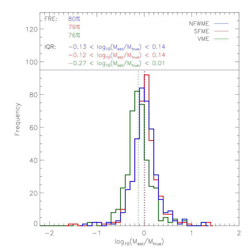
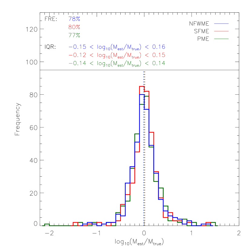
Figure 2: Histograms showing the ratio of the estimated mass to the true mass for the two different mass estimators. The left panel uses eqs. (6) and (9) applied to data sets of true distances and radial velocities. The right panel uses eqs. (10) and (12) applied to data sets of projected distances and los velocities. For the NFWME estimator, a concentration $c=17$ is assumed, which is typical for the haloes in the simulations. FRE and IQR are the fraction of reasonable estimates (FRE) and the inter-quartile range (IQR) as defined in the text. The means of the distributions are shown by vertical dotted lines, from which we see that the virial mass estimator is biased and underestimates the true mass (as originally pointed out by Bahcall & Tremaine 1981).

Table 1: Dwarf Spheroidal Masses

dSph		PME	SFME	NFWME
		($\times\ 10^{7}\ \mbox{M${}_{\sun}$}$)
Carina	($R<300\ \mbox{pc}$)	1.7	1.7	1.7
	($R<600\ \mbox{pc}$)	2.2	2.6	2.7
Fornax	($R<300\ \mbox{pc}$)	2.9	2.8	2.9
	($R<600\ \mbox{pc}$)	5.1	5.2	5.2
Sculptor	($R<300\ \mbox{pc}$)	1.8	1.8	1.8
	($R<600\ \mbox{pc}$)	2.5	3.1	3.0
Sextans	($R<300\ \mbox{pc}$)	1.3	1.3	1.3
	($R<600\ \mbox{pc}$)	2.0	2.2	2.2

Note. — All the error are $\pm 0.1\times 10^{7}\mbox{M${}_{\sun}$}$, taking into account the random measurement uncertainties only. For the NFWME, a concentration $c=30$ (typical for dSphs) has been assumed.

References

- Amorisco & Evans (2011) Amorisco, N., & Evans, N. W. 2011, MNRAS, in press (arXiv:1009.1813)
- An & Evans (2011) An, J. H., & Evans, N. W. 2011, MNRAS, in press (arXiv:1012.5180)
- Bahcall & Tremaine (1981) Bahcall, J. N., & Tremaine, S. 1981, ApJ, 244, 805
- Crain et al. (2009) Crain, R. A., et al. 2009, MNRAS, 399, 1773
- Deason et al. (2011) Deason, A. J., et al. 2011, MNRAS, submitted (arXiv:1101.0816)
- Heisler et al. (1985) Heisler, J., Tremaine, S., & Bahcall, J. N. 1985, ApJ, 298, 8
- Kleyna et al. (2002) Kleyna, J., et al. 2002, MNRAS, 330, 792
- Navarro et al. (1995) Navarro, J. F., Frenk, C. S., & White, S. D. M. 1995, MNRAS, 275, 720
- Springel et al. (2005) Springel, V., et al. 2005, Nature, 435, 629
- Strigari et al. (2008) Strigari, L. E., et al. 2008, Nature, 454, 1096
- Walker et al. (2009a) Walker, M. G., Mateo, M., & Olszewski, E. W. 2009a, AJ, 137, 3100
- Walker et al. (2009b) Walker, M. G., et al. 2009b, ApJ, 704, 1274
- Watkins et al. (2010) Watkins, L. L., Evans, N. W., & An, J. H. 2010, MNRAS, 406, 264
- Wilkinson et al. (2004) Wilkinson, M. I., et al. 2004, ApJ, 611, L21
- Wolf et al. (2010) Wolf, J., et al. 2010, MNRAS, 406, 1220