Sodium-oxygen anticorrelation and neutron capture elements in Omega Centauri stellar populations

Abstract

Omega Centauri is no longer the only globular cluster known to contain multiple stellar populations, yet it remains the most puzzling. Due to the extreme way in which the multiple stellar population phenomenon manifests in this cluster, it has been suggested that it may be the remnant of a larger stellar system. In this work, we present a spectroscopic investigation of the stellar populations hosted in the globular cluster $\omega$ Centauri to shed light on its, still puzzling, chemical enrichment history. With this aim we used FLAMES+GIRAFFE@VLT to observe 300 stars distributed along the multimodal red giant branch of this cluster, sampling with good statistics the stellar populations of different metallicities. We determined chemical abundances for Fe, Na, O, and $n$-capture elements Ba and La. We confirm that $\omega$ Centauri exhibits large star-to-star variations in iron with [Fe/H] ranging from $\sim-$2.0 to $\sim-$0.7 dex. Barium and lanthanum abundances of metal poor stars are correlated with iron, up to [Fe/H]$\sim-$1.5, while they are almost constant (or at least have only a moderate increase) in the more metal rich populations. There is an extended Na-O anticorrelation for stars with [Fe/H]$\lesssim-1.3$ while more metal rich stars are almost all Na-rich. Sodium was found to midly increase with iron over all the metallicity range.

1 Introduction

Omega Centauri ($\omega$ Cen) is one of the most studied and enigmatic stellar systems in our Galaxy. It hosts the most complex multiplicity of stellar populations observed in globular clusters (GC), with an anomalous large spread in [Fe/H], ranging from $\sim-$2.0 to $\sim-$0.6 dex (Norris, Freeman & Mighell 1996; Suntzeff & Kraft 1996; Lee et al. 1999; Pancino et al. 2000; Sollima et al. 2005a; Johnson et al. 2008; Johnson & Pilachowski 2010).

Evidence for large variations in the light elements among $\omega$ Cen stars at a given [Fe/H] was initially detected by Persson et al. (1980) in the form of a wide spread in CO absorption from infrared photometry. Brown & Wallerstein (1993) and Norris and Da Costa (1995) saw a similar variation in Na, Al and CNO elements. More recently, the variations in O, Na, and Al have been confirmed as well by spectroscopic studies conducted on a large sample of red giants (see Johnson & Pilachowski 2010, and reference therein).

Abundance ratios of slow neutron-capture process ($s$-process) elements relative to iron exhibit large star-to-star variations, with a significant number of stars showing enhancements over the entire metallicity range (Johnson & Pilachowski 2010 for red giants, and Stanford et al. 2007 for sub giant and main sequence stars). In addition, the ratio of $s$-process abundances to Fe increases with [Fe/H] for low [Fe/H], but becomes constant at higher [Fe/H] (Norris & Da Costa 1995; Smith, Cunha & Lambert 1995; Stanford, Da Costa & Norris 2010; Johnson & Pilachowski 2010).

The complexity of multiple stellar populations in $\omega$ Cen can also be seen in the multiple red-giant branches (RGB) and sub-giant branches (SGB) (Lee et al. 1999; Pancino et al. 2000; Ferraro et al. 2004; Sollima et al. 2005b; Bellini et al. 2009). Anderson (1997) and Bedin et al. (2004) clearly detected that the main sequence (MS) splits into two main branches. Contrary to any expectation from standard stellar evolutionary models, the more metal poor stars populate a redder MS (rMS), and stars at intermediate metallicity a bluer one (bMS; Piotto et al. 2005). To date, the only explanation we have to account for these observations is to assume a high overabundance of He for the bMS stars (Bedin et al. 2004; Norris 2004; Piotto et al. 2005). A third, less populated MS (MSa) has been discovered by Bedin et al. (2004) on the red side of the rMS and it has been associated with the most metal rich stars (Villanova et al. 2007). As well as bMS stars, the colors and the metallicity of the MSa are consistent with being populated by He rich stars (Norris  2004, Bellini et al. 2010).

All the observational data suggest that $\omega$ Cen has experienced a complex evolution with a still puzzling chemical enrichment history. As a matter of fact, we still do not know how such a large iron spread could have originated in a GC. For this reason, it has been suggested that $\omega$ Cen may not really be a GC, but may rather be the remnant of a larger system (Bekki & Norris 2006, and references therein).

Recent spectroscopic detections of intrinsic variations in [Fe/H] in the GCs NGC 6656 (M22, Marino et al. 2009), NGC 6715 (M54, Carretta at al. 2010), and Terzan 5 (Ferraro et al. 2009) suggest that $\omega$ Cen may not be a unique case, but rather may simply be an extreme example of a self-enriching cluster. While nearly all GCs studied to date show no significant variations in their $n$-capture elements (Ivans et al. 1999, 2001; James et al. 2004; Yong et al. 2008; Marino et al. 2008; D’Orazi et al. 2010), a bimodal distribution in the abundance of these elements has been detected in M22 (Marino et al. 2009), and NGC 1851 (Yong & Grundahl 2008) and has been associated with the bimodal SGB of these GCs. In particular, it appears that the nucleosynthetic enrichment processes in $\omega$ Cen and M22 were very similar (Da Costa & Marino 2010).

Omega Centauri is not completely dissimilar from mono-metallic globular clusters. Like all GCs studied so far, $\omega$ Cen stars show variations in light-element abundances, such as the well-known pattern of Na-O anticorrelation (Norris & Da Costa  1995, hereafter NDC95). It is now largely accepted that sodium and oxygen variations indicate the presence of different stellar populations in GCs, with a second generation enhanced in Na and depleted in O due to material that has undergone the entire CNO cycle in first generation stars (Ventura et al. 2001; Gratton et al. 2001; Gratton, Sneden & Carretta 2004). Proposed polluters to account for the Na-O anticorrelation observed in GCs are either AGB stars (D’Antona & Caloi 2004), fast rotating massive stars (Decressin et al. 2007), massive binaries (De Mink et al. 2009). At odds with these scenarios, an alternative model, recently proposed by Marcolini et al. (2009), considers as the first generation those stars that are O-depleted and Na-enhanced, while O-rich and Na-depleted stars should be formed successively after the self-pollution from SNe II. As observed for some GCs, the groups of stars with different Na and O can account for the distinct RGB sequences observed in the CMD (Marino et al. 2008, Milone et al. 2010). Hence the position of a star in the Na-O plane gives an important indication as to what population it belongs to. According to this, by homogeneously analyzing the Na-O anticorrelation in the largest sample of GC stars studied so far, Carretta et al. (2009), on the basis of their position on the Na-O plane, divided stars into primordial, intermediate, and extreme populations, confirming that the Na-O anticorrelation could be a useful tool to study multiple stellar population phenomenon in GCs.

In this article, we analyze a large sample of GIRAFFE@VLT spectra and determine chemical abundances of iron, sodium, oxygen, barium, lanthanum for hundreds of RGB stars in $\omega$ Cen. Thanks to this large sample of stars, we are also able to study the Na-O anticorrelation separately for stars in different metallicity populations.

The layout of this paper is as follows: Section 2 is a brief overview of the data set and the spectroscopic analysis; our results, and a comparison with previous studies, are presented in Section 3; Section 4 is a brief summary and discussion of the results obtained in this study.

2 Observations and data analysis

The data set consists of a large number of FLAMES/GIRAFFE spectra [proposals: 071.D-0217(A), 082.D-0424(A)] taken with the four set-ups HR09B, HR11, HR13, and HR15, which cover a spectral coverage of 5095-5404, 5597-5840, 6120-6405, 6607-6965 Å, respectively, with a resolution $R$ $\sim$ 20,000-25,000. The sample is composed by 300 red giants with a $V\leq$15. The typical S/N of the final combined spectra is $\sim$60-100, with values of S/N$\sim$130-160 in the spectral region around the O line at 6300 Å.

Data reduction involved bias-subtraction, flat-field correction, wavelength-calibration, sky-subtraction, and spectral rectification. To do this, we used the dedicated pipeline BLDRS v0.5.3, written at the Geneva Observatory (see http://girbld-rs.sourceforge.net). Chemical abundances were derived from a local thermodynamic equilibrium (LTE) analysis by using the spectral analysis code MOOG (Sneden 1973).

Atmospheric parameters (T_eff, log g, $\xi_{\rm t}$, metallicity) were estimated as follows. Effective temperatures (T_eff) were obtained via empirical relations of the $(V-K)$ colors with temperatures using the calibrations by Alonso, Arribas & Martínez-Roger (1999, 2001). We used $V$ magnitudes from Bellini et al. (2009), $K$ magnitudes retrieved from the Point Source Catalog of 2MASS (Skrutskie et al. 2006) and then transformed to the Carlos Sánchez Telescope photometric system, as in Alonso et al. (1999). As noted by Bellini et al. (2009), $\omega$ Cen is not significantly affected by differential reddening. This allowed us to apply a uniform reddening correction to all stars, by correcting our final $(V-K)$ colors for interstellar extinction using a $E(B-V)=$0.12 (Harris 1996) and $E(V-K)/E(B-V)=$2.70 (McCall 2004). At the end, as a test we verified that our adopted photometric temperatures satisfied excitation equilibrium by plotting the Fe I abundances versus the excitation potentials and verifying that they did not reveal any trends.

Surface gravities in terms of log g  were obtained from the apparent magnitudes, the above effective temperatures, assuming a mass M $=~{}0.80~{}{\rm{M_{\odot}}}$, bolometric corrections from Alonso et al. (1999), and a distance modulus of $(m-M)_{V}=$13.69 (Cassisi et al. 2009). Microturbolent velocities were determined by removing trends in the relation between abundances from neutral Fe lines and reduced equivalent widths (see Magain 1984). Final metallicities were then obtained interactively by interpolating the Kurucz (1993) grid of model atmospheres with T_eff, log g, and $\xi_{\rm t}$ fixed to find the [Fe/H] that best matched the Fe I lines.

Abundances from Fe lines were derived from equivalent-width (EW) measurements, but we derived the abundances for the other elements from spectral synthesis. The sodium content was determined from the doublet at $\sim$6150 Å. The oxygen abundances were derived from the forbidden line at 6300 Å, after the spectrum was cleaned from telluric contamination, using a synthetic spectrum covering the spectral region around the O line and taking line positions and EWs for the atmospheric lines of the Sun provided by Moore, Minnaert & Houtgast (1966). Barium was measured from the blended Ba II line at 6141 Å, and lanthanum from the two La II lines at 6262 Å and 6390 Å. The hyperfine splitting was taken into account for the La spectral lines by using data from Lawler, Bonvallet & Sneden (2001). Marino et al. (2008) provide more details on the linelist.

An error analysis was performed by varying the temperature, gravity, metallicity, microturbolence, and repeating the abundance analysis for stars representative of all the observed range in [Fe/H]. The parameters were varied by $\Delta$(T_eff)=$\pm$50 K, $\Delta$(log g)=$\pm$0.20 dex, $\Delta$($\xi_{\rm t}$)=$\pm$0.10 km/s and metallicity by $\pm$0.10 dex, which are typical internal uncertainties for stars with similar temperatures as ours and analyzed with spectra of similar quality (see Carretta et al. 2009). We redetermined the abundances by changing only one atmospheric parameter at a time for several stars, to see how abundances are sensitive to these variations in the atmospheric models. Changes in T_eff mostly affect the abundances derived from the subordinate ionization state transitions, i.e. Na I and Fe I abundances. On the contrary, abundances derived from the dominant ionization state transitions, i.e. singly ionized Ba, La, and Fe, and neutral O, are more sensitive to variations in gravity and metallicity. Errors introduced by changes in $\xi_{\rm t}$ increases with increasing metallicity. Assuming that the parameter uncertainties are uncorrelated, the resulting errors in chemical abundances were calculated by summing in quadrature with the contributions to errors given by each parameter. An additional source of internal errors for Fe chemical abundances is the uncertainty in the EW measurements, which we quantified to be $\sim$5 mÅ. We estimated this quantity by comparing EW measurements for the same spectral lines of pairs of stars with similar atmospheric parameters. In the case of Fe I this contribution is small since a large number of transitions (typically $\simeq$ 20-30) are available. We estimate the uncertainty in the [Fe/H] abundance from our EW measurements by assuming that the error will be $\sigma_{\rm EW}$/$\sqrt{N_{\rm lines}-1}$, where $\sigma_{\rm EW}$ is the dispersion in abundances and $N_{\rm lines}$ the number of spectral lines for a given specie. On average we estimated the EW error contribution to be $\sim$0.02 dex for Fe I, and $\sim$0.06 dex for Fe II. We summed these [Fe/H] uncertainties in quadrature to the uncertainties introduced by atmospheric parameters and found that typical internal errors in iron abundances are of the order of 0.05-0.07 dex for Fe I, and of $\sim$0.10 dex in the case of Fe II. For elements for which the abundances were derived from spectral synthesis, internal scatter factors are introduced by the errors in fitting the observed spectrum to the model, which included the fit to the continuum. For our spectra at relatively high S/N, this translates in typical uncertainties of $\sim$0.05 dex. The total uncertainty, which includes the error introduced by the uncertainties in the model atmosphere, obtained by repeating the spectral synthesis for different atmospheric parameters, as explained above, were estimated to be of the order of $\sim$0.10-0.15 dex in Ba and La, and of $\sim$0.10 in Na and O.

3 Results

In this Section we present our results for the five analyzed elements, that are of particular interest in the study of multiple stellar populations in $\omega$ Cen. The abundance ratios measured in this work, together with adopted atmospheric parameters, and $V$ magnitudes are listed in Tab.1, fully available in electronic form at the CDS (http://cdsweb.u-strasbg.fr).

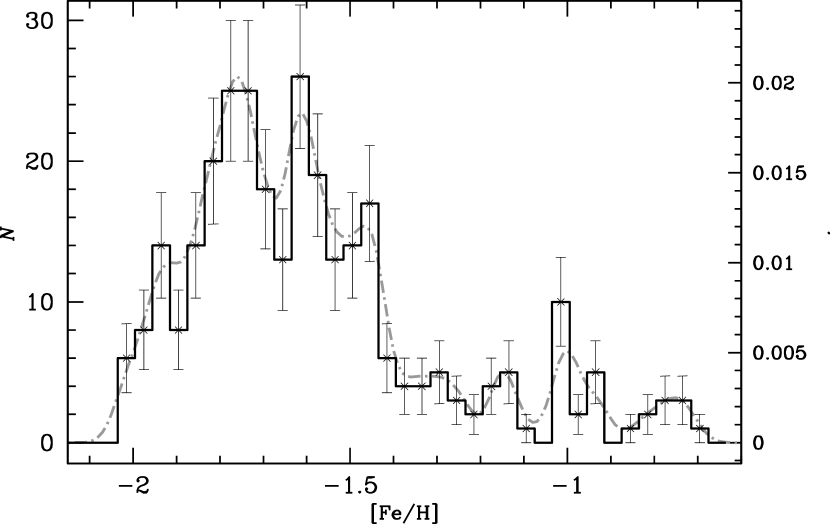
Figure 1: Histogram of [Fe/H] distribution. The superimposed dashed line represents the normalized kernel density distribution, the error bars are the Poisson errors.

1. Iron. We found that in $\omega$ Cen [Fe/H] ranges from $\sim-2.0$ to $\sim-$0.7 dex and follows the histogram distribution shown in Fig. 1, where error bars represent the Poisson errors. To estimate the significance of the revealed peaks, we smoothed the observed iron distribution with the normalized kernel density distribution $K=\sum_{i=1}^{N}e^{\frac{-(x-x(i))^{2}}{2\sigma^{2}}}$ (gray dot-dashed line superimposed to the observed histogram distribution) where: N is the number of stars for which the iron abundance has been determined in this paper, x(i) is the [Fe/H] measured for each star, x=[Fe/H], and $\sigma$ has been taken equal to 0.05 dex that is similar to the internal observational error associated with [Fe/H].

   The iron distribution represented in Fig. 1 is in agreement with previous studies, which have shown that stars in $\omega$ Cen span a wide interval in metallicity with almost no stars with [Fe/H]$<-$2.0, the majority having [Fe/H]$\sim-$1.7 and the remaining stars forming a tail at higher metallicities up to [Fe/H]$\sim-$0.7 (see Johnson et al. 2008; 2009; Johnson & Pilachowsky 2010, hereafter J08/09/10, and references therein).

   From a photometric analysis of the multimodal RGB, Sollima et al. (2005b) resolved five metallicity groups, going from the dominant RGB metal poor group with [Fe/H]$\sim-$1.7 to the more metal rich stars peaked at [Fe/H]$\sim-$0.7. A multimodal peak distribution was also found in Strömgren photometry by Calamida et al. (2009). The $\omega$ Cen metallicity distribution obtained from spectroscopic studies obviously depends on the sample statistics and on selection biases. Spectroscopic studies based on medium resolution data for large samples of $\omega$ Cen stars include: Sollima et al. (2005a, 250 SGB stars), Villanova et al. (2007, 80 SGB stars), and J08/09/10 (800 RGB stars in total). Sollima et al. (2005a) and J08/09/10 identified four groups of stars on the SGB and the RGB, respectively, peaked at values of [Fe/H]$\sim-$1.75, $-$1.45, $-$1.05, and $-$0.75 (values from J09), in agreement with the distributions obtained from RGB photometry (Sollima et al. 2005b). A similar distribution was found by Villanova and coworkers, but, possibly due to their lower statistics, they did not find stars in the more metal reach peak of Sollima et al. (2005a, b) associated with the fainter SGB (SGB-a).

   An inspection of Fig. 1 suggests that our metallicity distribution is consistent with the presence of multiple peaks corresponding to [Fe/H]=$-$1.75, $-$1.60, $-$1.45, $-$1.00, a broad distribution of stars extending between $-$1.40 and $-$1.00, and a tail of metal rich stars reaching values of [Fe/H]$\sim-$0.70. Interestingly, we also note a tail of stars at low metallicity down to [Fe/H]$\sim-$1.95, in agreement with calcium triplet low-resolution studies (Norris, Freeman, & Mighell 1996; Suntzeff & Kraft 1996) that have shown that there are a few RGB stars with [Fe/H] $<-$1.80. However, we note that, because of observational errors, particular caution should be adopted in the definition of multiple Fe peaks, and in establishing the presence of discrete populations rather than a Fe gradient in agreement with a prolonged star formation.

   Due to the target selection biases introduced by the necessity of having a sample representative of the entire range in metallicities, and to the presence of a radial metallicity gradient (J08 and references therein), our metallicity distribution cannot be considered to be representative of the distribution valid for the entire stellar populations in $\omega$ Cen.

2. Neutron capture elements. The abundances of Ba and La are plotted as a function of iron content in the panels ($a$) and ($b$) of Fig. 2. Both $n$-capture elements show a trend with iron. The abundance ratios of Ba and La increase with [Fe/H] from the most metal poor stars to [Fe/H]$\sim-$1.5 dex, while at higher metallicities the slope is is essentially flat. At high metallicities, the [La/Fe] shows less scatter than [Ba/Fe] probably due to an increase in scatter for Ba when the abundance gets high and the lines get too strong for an accurate abundance measurement.

   It should be noted that stars with [Fe/H]$\gtrsim-$1.5 belong to the metal intermediate RGB and RGB-a stars defined by Pancino et al. (2000). Radial distribution studies provide evidence that the blue MS and the metal intermediate RGB population are part of the same group of stars (Sollima et al. 2005b, Bellini et al. 2009), while RGB-a stars, which correspond to the progeny of MSa, exhibit a radial trend similar to the one observed for metal intermediate stars. From these considerations we could tentatively associate metal-poor/He-normal stars in $\omega$ Cen with stars in the metallicity range where La and Ba increase rapidly with iron, while metal-intermediate/He-rich stars (and maybe RGB-a stars) could correspond to the stars exhibiting a flatter trend of Ba and La with metallicity.

3. Sodium Our abundances show a large star-to-star Na variation, with [Na/Fe] going from less than $\sim-$0.3 in some of the most metal poor stars, to $\sim$1.2 in the metal rich populations. As shown in panel ($d$) of Fig. 2, sodium grows with iron but there are significant variations in [Na/Fe] among stars with the same [Fe/H]. Since we can compare stars with similar atmospheric parameters, we can safely assume that the observed Na variations are not due to departures from LTE. Non-LTE corrections have not been applied to our Na abundances because no standard values are provided in the literature. However, the Na transitions used here, for our metallicity range, typically have corrections $\leq$0.2 dex (e.g., Gratton et al. 1999; Gehren et al. 2004).

4. Oxygen The oxygen abundance ratio to iron ranges from $\sim-$0.6 to $\sim$0.9 dex. At variance with the other elements studied in this paper, there is no clear correlation with iron: a large spread is present at all metallicities.

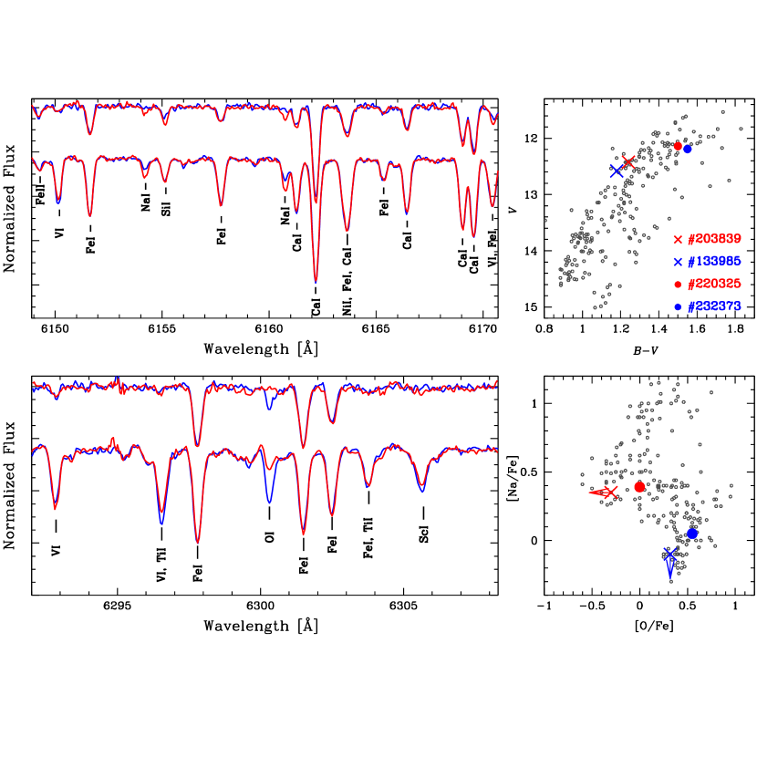
Figure 3: Spectra around Na (upper left panel) and O spectral lines (lower left panel) for two pairs of stars with similar atmospheric parameters: #203839 [T_eff=4371 K, log g=1.08, [A/H]=$-$1.83, $\xi_{\rm t}$=1.73 km/s] and #133985 [T_eff=4391 K, log g=1.16, [A/H]=$-$1.79, $\xi_{\rm t}$=1.60 km/s] are shown in the upper spectra, and #220325 [T_eff=4052 K, log g=0.73, [A/H]=$-$1.61, $\xi_{\rm t}$=1.90 km/s] and #232373 [T_eff=4093 K, log g=0.79, [A/H]=$-$1.58, $\xi_{\rm t}$=1.96 km/s] in the lower ones. The position of the two pairs of stars on the CMD and on the Na-O plane is shown on the right panels.

   A visual inspection of some spectra reinforces the impression that some stars that have the same iron abundances, strongly differ in their oxygen and sodium content. As an example, in Fig. 3 we show spectra of two pairs of stars with very similar stellar atmospheric parameters for which we measured a similar iron abundance but different oxygen and sodium. At variance with iron lines, the line depths of sodium (upper panel) and oxygen (lower panel) spectral lines differ significantly and, because of the similarity in their atmospheric parameters, must be indicative of an intrinsic difference in these elements. In the right panels of Fig. 3 we show the position of the two selected pairs of stars on the CMD (upper panel) and on the Na-O plane (lower panel): while each pair occupies a similar position on the CMD, the position on the Na-O plane suggests that the two stars in each pair belong to different stellar populations, given their different Na and O content.

3.1 Comparison with literature

In this Section we compare our atmospheric parameters and measured chemical abundances with previous analysis on $\omega$ Cen giants based on moderate and high resolution data.

Previous studies that used high-resoultion spectra or had large samples of RGB stars are: NDC95 (40 stars, $R$=38,000), J08/09/10 ($\sim$900 stars in total, $R$=13,000-18,000), Smith et al. (2000, 10 stars, $R$=35,000), Pancino et al. (2002, 6 stars, $R$=45,000), Brown et al. (1991, 18 stars, $R$=17,000).

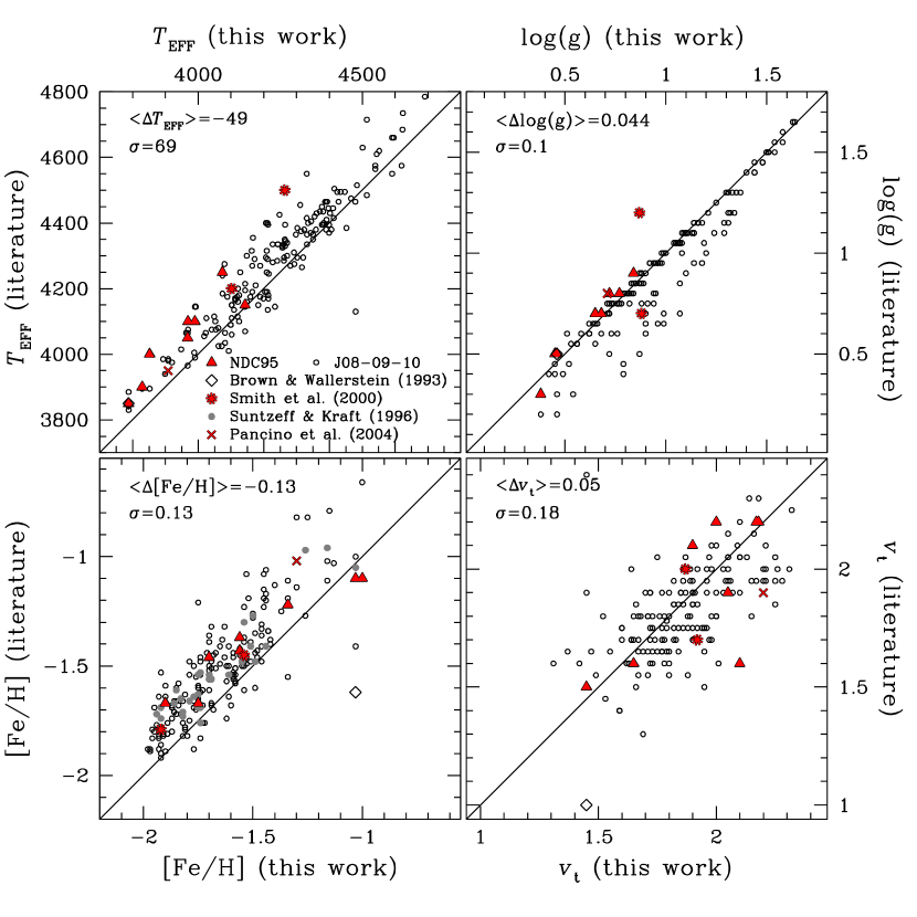
Figure 4: Comparison of the model atmosphere parameters adopted in this study vs. those available in the literature. A straight line indicates perfect agreement in all panels. Different symbols refer to data retrieved from different studies.

In Fig. 4 we compare our values for T_eff, log g, [Fe/H], and $\xi_{\rm t}$ with those of previous studies for stars in common with our sample. Data retrieved from different sources are represented with different symbols as indicated in the inset in the upper left panel. In addition to the works mentioned above, with gray dots, we represent metallicities from Suntzeff & Kraft (1996) derived from the Ca II infrared triplet and calibrated on the stars in common with NDC95. In all the panels we quoted the mean difference between our values and the literature ones, and the scatter of the points around the linear least squared fit with literature data. The straight line represents the perfect agreement.

An inspection of this figure suggests that a systematic difference of $\sim$0.15 dex in [Fe/H] is present between this study and the literature, our [Fe/H] is lower with a scatter around a linear least squared fit of $\sim$0.13 dex. Systematic differences are also present in the effective temperatures (left upper panel) with our temperatures on average lower by $\sim$70 K with respect to literature studies. As it can be seen from the figure, agreement is quite good for the surface gravity estimates, while there is a larger scatter for the microturbulence estimates.

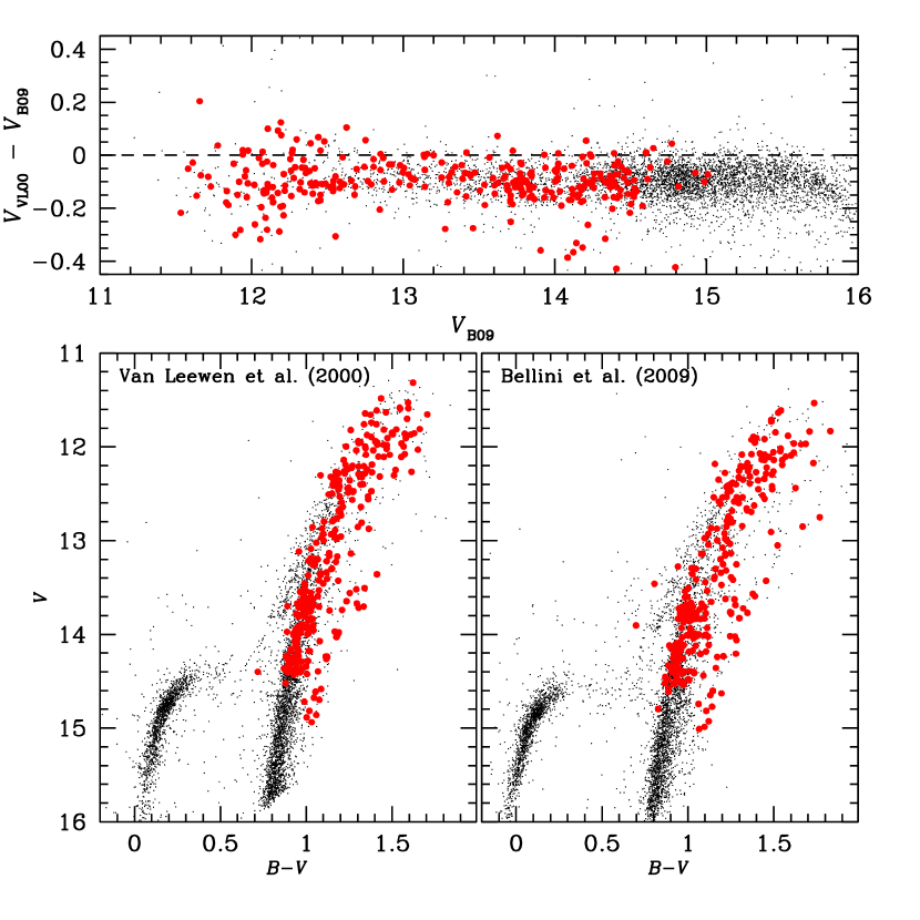
Figure 5: Upper Panel: Comparison of the $V$ magnitudes retrieved from Bellini et al. (2009) and from Van Leween et al. (2000). Lower Panels: $V$-$(B-V)$ CMDs constructed from the two different photometric catalogs. In all the panels the red points represent our spectroscopic sample.

It is not trivial to track down the cause of the offsets observed in the [Fe/H] and T_eff values, since different techniques have been used by different authors to derive temperatures. As fully explained in Section 2, we derived temperatures from the T_eff-$(V-K)$ calibration from Alonso et al. (1999). A similar method based on colors-T_eff calibrations was used by both NDC95 and J08/09/10. As an example, J09 averaged the T_eff values obtained from the color-temperature relations of Alonso et al. (1999, 2001) and Ramírez & Meléndez (2005) for $(V-J)$, $(V-H)$, and $(V-K)$ color indices, while J08 used only the $(V-K)$ colors and then adjusted temperatures to satisfy the excitation equilibrium for the Fe I lines. Since we used the same $K$ magnitudes retrieved from the 2MASS catalog as J08/09, possible differences in the $V$ magnitudes coming from different photometries could explain the differences that we observe with these authors. In Fig. 5 (upper panel), we compare $V$ magnitudes from the WFI photometry used in this study (Bellini et al. 2009, B09) with those from Van Leewen et al. (2000, VL00) used by J08/09. In the lower panels the two $V$-($B-V$) CMD are shown, with the stars studied in this work indicated by red symbols. The comparison between the two photometries clearly shows that on average $V_{B09}-V_{VL00}\sim-$ 0.15. These differences help to explain why our temperatures are systematically lower by $\sim$50-100 K, and hence contribute to produce a systematic difference in the measured metallicities. Our final choice is to use the $V$ magnitude from B09 considered to be more reliable because these values are corrected for sky concentration effects and calibrated on Stetson photometric secondary standards (Stetson 2000, 2005). We concluded that even if systematic differences in the metallicities are present with previous studies, they will not impact our investigation, since we are mainly interested in the star-to-star variations, which are differential measurements.

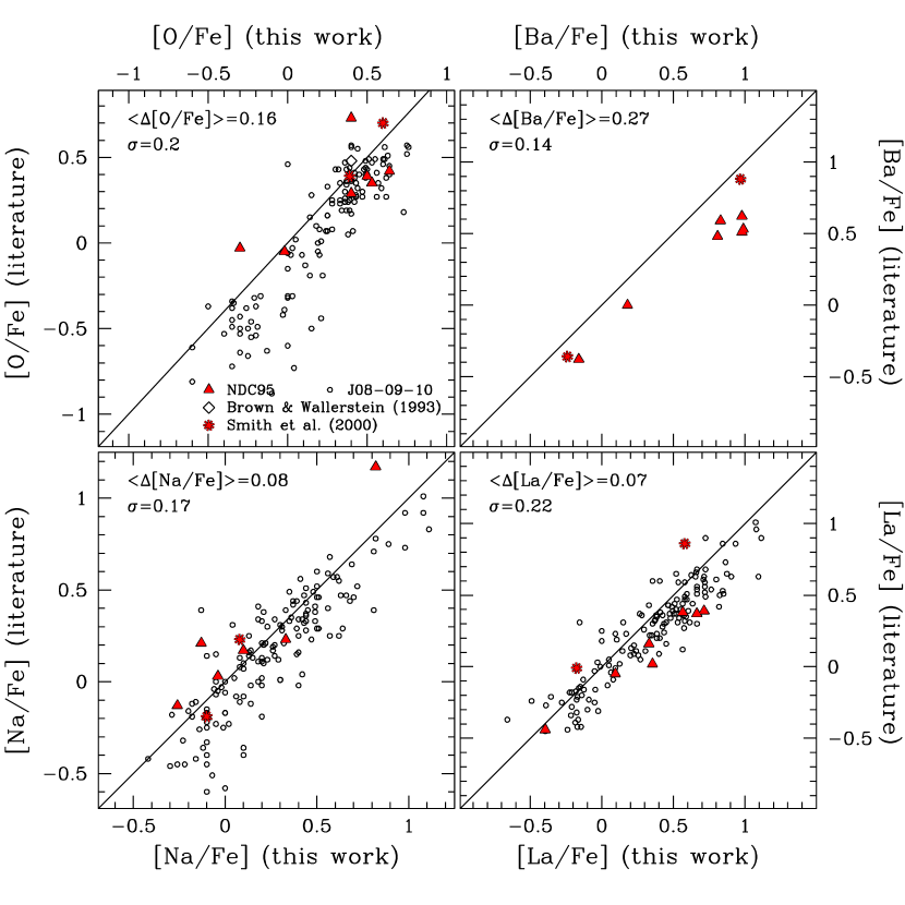
Figure 6: Comparison of the abundance ratios obtained in this study vs. those available in the literature. A straight line indicates perfect agreement in all panels. Different symbols refer to data retrieved from different studies.

In Fig. 6 we compare the elemental abundance ratios obtained in this work with those obtained in the other studies. As it can be seen from the figure, [O/Fe], [Na/Fe], and [La/Fe] abundances are in reasonable agreement with literature values, indicating that these abundance ratios are less affected by systematic differences in the atmospheric parameters. Larger systematic discrepancies are present for the [Ba/Fe] abundances, for which however literature values on RGB are available only in NDC95 and Smith et al. (2000).

3.2 Sodium oxygen anticorrelation

In this Section we analyze the Na-O anticorrelation and attempt to further analyze the behaviour of sodium and oxygen in stars with different iron. Specifically, we analyzed the 253 out of 300 stars, for which we were able to derive reliable Na and O contents. In some cases, we were able to give only an upper limit for the Na and O abundances.

On the CMD of $\omega$ Cen at least 5 distinct sequences can be recognized, with hints for the possible existence of other, less populous components (Sollima et al. 2005b; Bellini et al. 2010). If we hope to understand the sequence of events that led to the formation of this puzzling cluster and its present state, it will be critical to determine whether spreads and correlations in abundance patters are present only between sub-populations, or whether they are present within the sub-populations themselves. Indeed, if sub-populations are found to be chemically homogeneous this would indicate that star-formation proceeded as a series of bursts, interleaved by inactive periods during which the ejecta of intermediate mass stars were accumulating, prior to a successive burst. On the other hand, if each sub-population was to exhibit abundance spreads, then accumulation of stellar ejecta, hypothetical dilution with pristine material, and star formation had to proceed simultaneously. We know that the different metallicity of the rMS and bMS imply that the helium abundance has at least two discrete values, as opposed to a continuous distribution, and therefore it would be difficult to envisage a process that would lead to a large spread in oxygen without producing a spread also in helium.

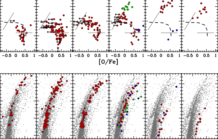
Figure 8: Lower panels: $V$ vs. $(B-V)$ CMD from WFI photometry (Bellini et al. 2009). In each panel, the red dots show stars which have been selected according to their metal content (as indicated in the inset of the corresponding upper panel). Upper panels: estimated [O/Fe] and [Na/Fe] for the stars of each metallicity group. A fiducial, traced by hand on the Na-O anticorrelation for stars with $-$1.65$\leq$[Fe/H]$<-$1.50, has been over-imposed to each Na-O plane. In the fourth and fifth panels, the green and blue dots highlight the position in the CMD of the stars with extreme values in the Na-O anticorrelation, as represented in the corresponding upper panels.

One first difficulty in attempting this approach is encountered when trying to identify each of the sub-populations on the CMD. This is more easy on high S/N Hubble Space Telescope (HST) images (see, e.g. the CMD from high precision Wide Field Camera 3 (WFC3) photometry in Bellini et al. 2010). However, HST data cover relatively small, and crowded, areas of the cluster, much smaller than the 25 arcmin diameter field of view of the FLAMES facility that we have used. Therefore, we have been forced to select our targets on a CMD based on wide field images taken at the ESO/MPI 2.2m telescope, where the distinction of the various RGBs is not as clean (see bottom panel of Fig. 8). Therefore, in this paper, we separated the different RGB sub-populations only on the basis of their iron abundance.

We also note that, unlike other clusters with prominent multiple populations (e.g., NGC 2808), $\omega$ Cen exhibits the very wide and complex distribution of iron abundances shown in Fig. 1. Thus, while in other clusters, sub-populations formed out of materials that were enriched by AGB ejecta, in $\omega$ Cen the sub-populations experienced enrichment by SN products as well. This, of course, does not preclude the possibility that –as in other clusters –some sub-populations may have the same iron abundance and different sodium and oxygen abundances. This is to say that iron alone may not suffice to identify all $\omega$ Cen sub-populations, as indeed it does not suffice for most other clusters.

In addition, we should consider that the large variations in He abundance present in $\omega$ Cen could have a significant effect on the transformation from [Fe/H] into metal content, due to the not negligible variations in the H content. A similar effect has been noticed by Bragaglia et al. (2010) in the case of NGC 2808, where a difference of about 0.07 dex in [Fe/H] was obtained between the Na- (and likely) He-poor population (found more metal-poor), and the Na- and He-rich population: this difference can be entirely attributed to a variation in the H content from $X\sim 0.75$ down to $X\sim 0.64$, which corresponds to 0.07 dex. Since the range of He abundances is similar in $\omega$ Cen and NGC 2808, we should consider that the metal content of the He-rich population is likely to be slightly overestimated with respect to that of the He-poor population when [Fe/H] is used as a metal abundance index.

To study the behaviour of the Na-O anticorrelation in $\omega$ Cen, we first divided our sample into three broad groups, following Villanova et al. (2007): i) a metal poor one with [Fe/H]$\leq-1.5$ (MP); ii) an intermediate-metallicity group with $-1.5<$[Fe/H]$\leq-1.2$ (MInt); and iii) a metal rich (MR) group formed by stars with [Fe/H]$>-1.2$.

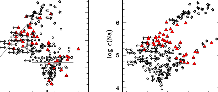
Figure 7: Na-O anticorrelation for 253 stars. We have used open circles, filled red triangles and open stars to represent stars with [Fe/H]$\leq-$1.50 (MP stars), $-$1.50$<$[Fe/H]$\leq$1.20 (MInt stars), and [Fe/H]$>-$1.20 (MR stars) respectively.

The Na and O abundances for our sample of stars in the Na-O plane are shown in the two panels of Fig. 7. On the left panel we represent the Na and O abundance ratios relative to iron. The two grey lines separate the three regions on the Na-O plane occupied by the primordial (region at high O and low Na), intermediate (region delimited by the two lines), and extreme (region at low O and high Na delimited by the oblique line) populations as defined by Carretta et al. (2009). Note that these three populations identified on the basis of the position on the Na-O plane, have been defined for normal mono-metallic GCs. Obviously, in the case of $\omega$ Cen it is more difficult to separate three groups of stars on these basis, not only because of the spread in iron, but also because a significant number of stars lies in anomalous positions with respect to the three regions of Carretta et al. (2009). On the right panel the Na-O anticorrelation has been also represented in the log$\epsilon$(Na)-log$\epsilon$(O) plane. In both panels, MP and MInt stars are plotted as open circles and red triangles respectively, while MR stars are represented as open stars. We immediately note that a Na-O anticorrelation is present within almost all $\omega$ Cen sub-populations, although with a large dispersion both in Na and O, and with a fraction of stars with abundances [Na/Fe]$\gtrsim$0.8 occupying an apparently anomalous (with respect to the other GCs) position on the Na-O plane. Both the MP and MInt groups exhibit the Na-O anticorrelation with MInt stars having, on average, lower oxygen abundance and higher sodium. Apparently, no strong evidence for a Na-O anticorrelation has been found for stars with [Fe/H]$>-$1.2. Almost all the stars in this metal rich group are Na rich, and the sample spans a large range in O.

As previously discussed, our results confirm that $\omega$ Cen could host more than three groups of stars with different iron. An inspection of Fig. 1 shows that the metallicity distribution has multiple “peaks” at [Fe/H]$\sim-$1.95, $-$1.75, $-$1.60, $-$1.45, and $-$1.00, and one at $-0.75$. It is impossible to assess whether these peaks can define six distinct stellar groups, each with a different iron abundance. In any case, our purpose here is simply to analyze the behaviour of the Na-O anticorrelation as iron increases. To further investigate the Na-O anticorrelation properties in $\omega$ Cen sub-populations, in Fig. 8, we arbitrarily isolated six groups of stars around the iron peaks mentioned above. The exact interval of [Fe/H] corresponding to each group is quoted in the upper panels, where we show the Na-O anticorrelation for stars in each selected group. This procedure by no means guarantees that sub-populations have been correctly isolated from each other, and contamination across adjacent bins must certainly exist given the $\sim 0.10$ dex 1$\sigma$ error in [Fe/H]. This diffusion of stars in and out each bin has to be taken in full account when discussing the chemical abundances of stars within each of the [Fe/H] bins discussed below. In all the panels the selected stars in the various Fe bins are represented as red points, and the two grey lines are as in Fig. 7. Lower panels of Fig. 8 show the position in the V vs. B$-$V CMD of stars in the corresponding iron interval. In order to better follow the trend of the Na-O anticorrelation as iron increases, we plot in each panel a fiducial line, drawn by hand, tracing the anticorrelation for the population with $-$1.65$\leq$[Fe/H]$<-$1.50 (third panel from the left). The Na-O anticorrelation is present over a wide metallicity range. It is interesting to note that, when we compare the Na-O anticorrlation in each panel agains the fiducial line, the average Na level (abundance) increases systematically as we go from the metal-poor to the metal-rich populations.

The fraction of stars with low and intermediate O content also increases with metallicity. The Na-O anticorrelation disappears for stars with [Fe/H]$\gtrsim-$1.05, where most of the stars occupy a quite anomalous portion of the Na-O plane, at high Na abundance and with large spread in O. In green and blue symbols we highlight the position of stars with an anomalous position on the Na-O plane with respect to the bulk of stars in their arbitrary metallicity bins (possibly due to errors in [Fe/H] measurements which causes the migration of stars in adjacent bins). The corresponding position of these stars on the CMD is also shown in the lower panels with the same colors as in the upper panels.

We now discuss the properties of stars in each bin in more detail.

Bin 1, [Fe/H] $<-1.9$, the most metal poor component. This very metal poor group does not appear in the Sollima et al. (2005b) photometric metallicity distribution, most likely because the color is saturated below [Fe/H]$\sim-1.65$. However, some hint of a peak in the metallicity distribution among values of $-$1.8 and $-$1.9, is present in the Strömgren photometry-based study by Calamida et al. (2009). This low-iron peak in Fig. 1 may or may not be an extension of the main peak at [Fe/H]=$-$1.75, reaching more than $\sim 2\sigma$ away from it. We assume this peak to be a real, very metal poor component, with most stars showing primordial Na and O abundances, i.e., high oxygen and low sodium. Two or three O-poor stars may well belong to the next bin, so it appears likely that this group is chemically homogeneous as far as iron and oxygen are concerned, possibly with a spread only in sodium.

Bin 2, $-1.90\leq$[Fe/H] $<-1.65$, this is the main iron-poor group, and these red giants are assumed to be the progeny of the rMS, i.e., the main first generation. However, many stars have high sodium and low oxygen, and therefore, being made of materials that have been highly processed through the CNO-cycle and proton-capture reactions, cannot belong to the first generation. We consider it more likely that this group actually consists of a mixture of first and second generation stars, i.e., the progeny of both the rMS and the bMS stars, with the latter ones having possibly migrated to this [Fe/H] bin from the next adjacent bin whose width is only marginally larger that our internal error in [Fe/H]. Still, as in the previous bin, sodium abundances extend significantly above the limit for the field stars.

Bin 3, $-1.65\leq$[Fe/H] $<-1.50$, this [Fe/H] peak should correspond to the bMS, i.e., the main helium-rich second generation component. Indeed, most stars are oxygen poor and sodium rich, as expected for the high helium sub-population. Just a few stars appear to have the primordial composition (oxygen rich, sodium poor), and it is likely that these may have migrated from Bin 2. Given the narrowness of this bin, it is expected that there will be both contamination from and loss to adjacent bins, and we conclude that its main component, oxygen poor and sodium rich, may be homogeneous in these elements. However, as shown in Fig. 3, this bin includes stars with indistinguishable [Fe/H], but different sodium and oxygen, indicating that there must be a component that has formed out of CNO-processed material not further enriched in iron.

Bin 4, $-1.50\leq$[Fe/H] $<-1.05$, this is the broadest of all bins, and likely consists of 2 or 3 minor sub-populations. The distinct oxygen-poor, sodium-rich group could be a contaminant from the previous bin (and being made of bMS progeny), and it may be homogeneous in these elements. One group with intermediate oxygen and very high sodium is clearly distinct from the others, and looks homogeneous. More puzzling is the group with near-pristine oxygen and sodium, unlikely to represent objects migrated from Bin 2 because of errors in [Fe/H]. Some stars in this bin likely represent the RGB progeny of the so-called anomalous Main Sequence (MSa). Indeed, stars highlighted in blue and green, which lie well outside the conventional Na-O anticorrelation (dashed line), also occupy a different region on the CMD with respect to the bulk of stars present in this bin and represented in red. These stars appear to be distributed between the RGB sequence defined by the red stars in this bin and the RGBa of Pancino et al. (2000). Note that the group with intermediate oxygen and very high sodium, represented by green symbols, is clearly distinct from the others, and looks homogeneous. Overall, this bin includes at least three fairly distinct groups, each being possibly chemically homogeneous.

Bin 5, $-1.05\leq$[Fe/H] $<-0.90$, this is a very narrow bin, and is dominated by the very high sodium, intermediate-oxygen stars already found in the previous bin, together with three stars with apparently pristine oxygen and sodium to iron ratios. Being so narrow in [Fe/H], it is likely that this bin has lost stars to the two adjacent bins, where indeed this very sodium-rich population is also found. The three stars with low Na and high O, represented in blue, may have diffused from the previous iron bin, and also their position on the CMD appears to be slightly on the blue side of the RGBa, rather than belong to the RGBa itself.

Bin 6, [Fe/H] $\geq-0.90$, photometrically, this iron-rich group looks essentially identical to the main component in the previous group (see also lower panels in Fig. 8), and like the previous group, it represents the RGBa progeny of MSa stars. One may argue that the very high-sodium stars in the last three bins are essentially identical. However, there appears to be a possible trend of increasing [O/Fe] with increasing [Fe/H], i.e. a systematic increase of [O/Fe] from Bin 4 to Bin 6. Alternatively, this extreme (MSa) population may actually exhibit a spread in both [Fe/H] and [O/Fe], with oxygen increasing more rapidly than iron, quite an odd behaviour if most of iron comes from Type Ia supernovae and most oxygen comes from core collapse supernovae. However, in the high resolution CMD from WFC3 data of Bellini et al. (2010), the MSa is clearly spread into two sequences, which evolve into two distinct SGBs. Therefore, the [O/Fe] differences among the very high sodium stars in Bins 4-6 may well be real, and the result of having the two components of the MSa population being spread in various proportions among these [Fe/H] bins. Again, this group of sodium-rich stars is completely out of the conventional sodium-oxygen anticorrelation.

This analysis of the oxygen and sodium abundances in the various iron bins can be summarized as follows:

1. None of the iron bins appears to isolate one single sub-population, except perhaps Bin 6. However, this is possibly due to diffusion from adjacent bins,

2. The data are consistent with each [Fe/H] bin containing 1 to 3 distinct sub-populations, each being homogeneous in iron and oxygen abundance, while possibly exhibiting a modest spread in sodium.

3. In the three most metal rich bins there is a sodium rich component that does not follow the conventional Na-O anticorrelation, with actually a hint for a Na-O correlation (cf. also Fig. 7).

4. Analysis of individual stars shows that in some cases there is no one-to-one correspondence between [Fe/H] and the sodium and oxygen abundances, i.e., some stars exist that have virtually identical iron but very different sodium and oxygen (see panels c and d in Fig. 2 and Fig. 3). This is certainly not unique to $\omega$ Cen, as indeed most clusters exhibit a single iron abundance while hosting stars with different oxygen and sodium abundances.

4 Discussion

In this paper, we have presented Na, O, Ba and La abundances, in a large, homogeneously analyzed sample of $\omega$ Cen RGB stars. These measurements allowed us to study, with a large sample of stars, the chemical pattern of different metallicity groups hosted by the cluster.

From our results, the picture of the chemical enrichment history in $\omega$ Cen turns out to be even more complicated than previously thought:

• We confirm that $\omega$ Cen exhibits large star-to-star variations in iron, with [Fe/H] ranging from $\sim-$2.0 to $\sim-$0.7 dex. The iron distribution is characterized by several peaks that can clearly be associated with stellar groups located in different RGB regions.

• Barium and lanthanum increase with iron for stars with [Fe/H]$\lesssim-$1.5, while their abundance distribution is flatter for the more metal rich populations ([Fe/H]$\gtrsim-$1.5).

• The Na-O anticorrelation is present among $\omega$ Cen stars (as first found by NDC95). The presence of stars defining a Na-O anticorrelation has been detected over almost all the observed metallicity range, but with differences in the fractions of primordial, intermediate and extreme population stars. The metal poor bin (with [Fe/H]$\lesssim-$1.9) hosts a large fraction of stars whose Na and O abundances resemble that of the halo field stars (primordial population), i.e. they are O rich and Na poor. As the metallicity increases, the percentage of the Na rich and O poor stars becomes larger, resulting in a Na-O anticorrelation more extended than the one observed in the metal poor regime. This result is relevant for an understanding of the formation of the different stellar populations in $\omega$ Cen, and similar, though much more complex than what found in M54 by Carretta et al. (2010). Interesting, the presence of a Na-O anticorrelation has also been found in the two metallicity groups hosted in M22 (Marino et al. 2009; Marino et al. in prep.). In $\omega$ Cen the anticorrelation disappears for the most metal rich populations.

The runs of barium and lanthanum abundances with [Fe/H] provide further (puzzling) information on the chemical enrichment history of $\omega$ Cen. Notice that such a fast raise of $s$-process increase with iron shown in Fig. 2 is not found in other galactic environments, as shown in Fig.17 of J10. A rise in the $s$-process elements has been observed in some dwarf spheroidal (see Tolstoy, Hill & Tosi 2009). However, differently from $\omega$ Cen whose stars show enhanced [$\alpha$/Fe] ratios, dwarf galaxies exhibit low [X/Fe] ratios for the light and especially $\alpha$ elements (Venn et al. 2004; Geisler et al. 2007) suggesting a significant contribution from Type Ia SNe. In addition, in dwarf spheroidals high levels of Ba and La are reached at a much higher metallicity than in $\omega$ Cen.

Ba and La are produced by $n$-capture processes, either $s$- or $r$-processes. Smith et al. (2000) and J10 found that Ba and La in $\omega$ Cen metal-rich stars should be produced mainly by the $s$-process, because Eu (whose fractional contribution by $s$-process is of only $\sim$3%, Simmerer et al. 2004) abundances are roughly constant, independently of [Fe/H], ruling out the $r$-process as an important contributor. In the Sun, the $s$-process contribution is mainly due to two components: the main component (attributed to low mass AGB stars of 1.5–3 M_⊙, Busso, Gallino & Wasserburg 1999), and the weak component (attributed to massive stars, see Raiteri et al. 1993, and references therein). At solar metallicity, this last component mainly produces the lighter $s$-process nuclei, at most up to Sr and Kr (Raiteri et al. 1993). However, in a metal poor, and expecially $\alpha$-element enhanced environment more neutrons are produced per iron seed nucleous, and heavier $s$-process elements are likely to be produced. Hence, the neutron seed is the $\rm{{}^{22}Ne(a,n)}{{}^{25}Mg}$ reaction, and in an $\alpha$-enhanced environment more O (and Ne) are present to start with per iron seed. It remains to be seen whether the models can produce elements as heavy as Ba and La in stellar environments characterized by the chemical abundances observed in $\omega$ Cen. The low abundance of Cu in [Fe/H]$\sim-1.0$ stars in $\omega$ Cen (Cunha et al. 2002; Pancino et al. 2002) may argue against a large contribution by the weak component, although with a higher neutron-to-iron ratio one expect the weak component to be shifted towards heavier nuclei.

As suggested by the referee, an additional possibility could be to allow for rotating massive stars. Rotational mixing may drive some protons into the He-burning region, allowing for a primary contribution from the ne22(a,n) source, see for e.g., the preliminary models by Pignatari et al. (2008). Obviously more detailed models are required to test this.

Alternatively, or in addition, the Ba and La enhancements could come from the main component by the more massive AGB stars ($M\gtrsim 3~{}M_{\odot}$), (where the $\rm{{}^{22}Ne(a,n)}$ is also partly primary as well). The less massive AGB stars represent a well identified nucleosynthetic site to produce $s$-elements, via the $\rm{}^{13}C(a,n)^{16}O$ reaction. An advantage of these stars in reproducing the chemical pattern observed in $\omega$ Cen, is that the neutron flux increases with iron seed with decreasing metallicity. However, these less massive AGB stars have the important disadvantage that they would require a very long timescale for this $s$-process enrichment (on the order of a Gyr), which would be difficult to reconcile with the other relevant chemical-enrichment timescales set by the massive AGB stars ($\sim 3-8~{}M_{\odot}$, D’Antona & Caloi 2004) and by the iron and $\alpha$-element enrichment ($>8~{}M_{\odot}$ stars). Thus, it seems more likely to us that the $s$-process elements in $\omega$ Cen were produced by the same massive SN and AGB stars that were responsible for the enrichment of iron, $\alpha$-elements, and helium and for establishing the Na-O anticorrelation, than to assume that $s$-process ehnancement comes from a third set of producers, such as low-mass AGB stars.

Acknowledgements We warmly thank the anonymous referee whose suggestions helped to improve the paper. The authors acknowledge support by PRIN2007 (prot. n. 20075TP5K9), and by ASI under the program ASI-INAF I/016/07/0. A.B. acknowledges support by the CA.RI.PA.RO. foundation, and by the STScI under the ”2008 Graduate Research Assistantship” program.

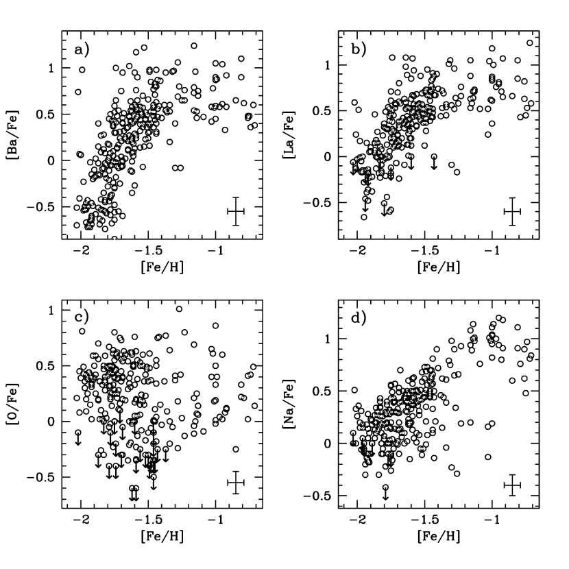
Figure 2: Upper panels: abundance ratios for the two $n$-capture elements Ba and La relative to Fe as a function of [Fe/H]. Lower panels: abundance ratios for the $p$-capture elements O and Na relative to Fe as a function of [Fe/H].

Table 1: Coordinates RA and DEC, $V$ magnitude, adopted atmospheric parameters and measured abundance ratios for the 300 stars in $\omega$ Cen. The complete table is available only in electronic form at CDS.

ID	RA	DEC	$V$	Teff [K]	log g	$\xi_{\rm t}$ [km/s]	[Fe/H]	[O/Fe]	[Na/Fe]	[Ba/Fe]	[La/Fe]
109369	201.818386	$-$47.549133	13.044	4544	1.44	1.70	$-$1.43	0.75	$-$0.14	0.56	0.00
112383	201.834424	$-$47.534160	12.850	4359	1.24	1.65	$-$1.62	0.62	0.20	0.40	0.36
114842	201.817052	$-$47.522465	12.927	4415	1.31	1.52	$-$1.90	0.39	0.23	$-$0.10	0.06
116394	201.846235	$-$47.515000	13.777	4663	1.80	1.35	$-$1.71	0.10	0.30	0.24	$-$0.07
119799	201.830431	$-$47.499341	14.023	4293	1.67	1.40	$-$0.71	0.14	0.84	0.38	0.58
120847	201.807438	$-$47.494576	13.034	4343	1.31	1.55	$-$1.51	0.47	0.44	0.49	0.47
121048	201.834524	$-$47.493559	13.781	4394	1.64	1.48	$-$1.16	0.69	0.20	0.54	0.53
126851	201.854789	$-$47.466319	14.061	4274	1.67	1.55	$-$0.72	0.49	0.81	0.60	1.24
131171	201.849422	$-$47.445934	13.760	4648	1.78	1.60	$-$1.85	$\cdots$	$\cdots$	$-$0.42	$\cdots$
131256	201.823805	$-$47.445611	13.407	4428	1.51	1.53	$-$1.34	$-$0.20	0.39	0.53	0.57

References

- Alonso et al. (1999) Alonso, A., Arribas, S., & Martínez-Roger, C. 1999, A&AS, 140, 261
- Alonso et al. (2001) Alonso, A., Arribas, S., & Martínez-Roger, C. 2001, A&A, 376, 1039
- Anderson (1997) Anderson, A. J. 1997, Ph.D. Thesis
- Bedin et al. (2004) Bedin, L. R., Piotto, G., Anderson, J., Cassisi, S., King, I. R., Momany, Y., & Carraro, G. 2004, ApJ, 605, L125
- Bekki & Norris (2006) Bekki, K., & Norris, J. E. 2006, ApJ, 637, L109
- Bellini et al. (2009) Bellini, A., Piotto, G., Bedin, L. R., King, I. R., Anderson, J., Milone, A. P., & Momany, Y. 2009, A&A, 507, 1393
- Bellini et al. (2010) Bellini, A., Bedin, L. R., Piotto, G., Milone, A. P., Marino, A. F., & Villanova, S. 2010, AJ, 140, 631
- Brown et al. (1991) Brown, J. A., Wallerstein, G., Cunha, K., & Smith, V. V. 1991, A&A, 249, L13
- Brown & Wallerstein (1993) Brown, J. A., & Wallerstein, G. 1993, AJ, 106, 133
- Busso et al. (1999) Busso, M., Gallino, R., & Wasserburg, G. J. 1999, ARA&A, 37, 239
- Calamida et al. (2009) Calamida, A., et al. 2009, ApJ, 706, 1277
- Carretta et al. (2009) Carretta, E., et al. 2009, A&A, 505, 117
- Carretta et al. (2010) Carretta, E., et al. 2010, ApJ, 714, L7
- Cassisi et al. (2009) Cassisi, S., Salaris, M., Anderson, J., Piotto, G., Pietrinferni, A., Milone, A., Bellini, A., & Bedin, L. R. 2009, ApJ, 702, 1530
- (15) Cunha, K., Smith, V. V., Suntzeff, N. B., Norris, J. E., Da Costa, G. S., & Plez, B. 2002, AJ, 124, 379
- Da Costa & Marino (2010) Da Costa, G. S., & Marino, A. F. 2010, arXiv:1009.1955
- D’Antona & Caloi (2004) D’Antona, F., & Caloi, V. 2004, ApJ, 611, 871
- Decressin et al. (2007) Decressin, T., Meynet, G., Charbonnel, C., Prantzos, N., & Ekström, S. 2007, A&A, 464, 1029
- de Mink et al. (2009) de Mink, S. E., Pols, O. R., Langer, N., & Izzard, R. G. 2009, A&A, 507, L1
- D’Orazi et al. (2010) D’Orazi, V., Gratton, R., Lucatello, S., Carretta, E., Bragaglia, A., & Marino, A. F. 2010, ApJ, 719, L213
- Ferraro et al. (2004) Ferraro, F. R., Sollima, A., Pancino, E., Bellazzini, M., Straniero, O., Origlia, L., & Cool, A. M. 2004, ApJ, 603, L81
- Geisler et al. (2007) Geisler, D., Wallerstein, G., Smith, V. V., & Casetti-Dinescu, D. I. 2007, PASP, 119, 939
- Gehren et al. (2004) Gehren, T., Liang, Y. C., Shi, J. R., Zhang, H. W., & Zhao, G. 2004, A&A, 413, 1045
- Gratton et al. (1999) Gratton, R. G., Carretta, E., Eriksson, K., & Gustafsson, B. 1999, A&A, 350, 955
- Gratton et al. (2001) Gratton, R. G., et al. 2001, A&A, 369, 87
- Gratton et al. (2004) Gratton, R., Sneden, C., & Carretta, E. 2004, ARA&A, 42, 385
- Harris (1996) Harris, W. E. 1996, AJ, 112, 1487
- Ivans et al. (1999) Ivans, I. I., Sneden, C., Kraft, R. P., Suntzeff, N. B., Smith, V. V., Langer, G. E., & Fulbright, J. P. 1999, AJ, 118, 1273
- (29) Ivans, I., Kraft, R.P., Sneden, C., et al. 2001, AJ, 122, 1438
- James et al. (2004) James, G., et al. 2004, A&A, 414, 1071
- Johnson et al. (2008) Johnson, C. I., Pilachowski, C. A., Simmerer, J., & Schwenk, D. 2008, ApJ, 681, 1505
- Johnson et al. (2009) Johnson, C. I., Pilachowski, C. A., Michael Rich, R., & Fulbright, J. P. 2009, ApJ, 698, 2048
- Johnson & Pilachowski (2010) Johnson, C. I., & Pilachowski, C. A. 2010, ApJ, 722, 1373
- Lawler et al. (2001) Lawler, J. E., Bonvallet, G., & Sneden, C. 2001, ApJ, 556, 452
- Lee et al. (1999) Lee, Y.-W., Joo, J.-M., Sohn, Y.-J., Rey, S.-C., Lee, H.-C., & Walker, A. R. 1999, Nature, 402, 55
- Magain (1984) Magain, P. 1984, A&A, 134, 189
- Marcolini et al. (2009) Marcolini, A., Gibson, B. K., Karakas, A. I., & Sánchez-Blázquez, P. 2009, MNRAS, 395, 719
- Marino et al. (2008) Marino, A. F., Villanova, S., Piotto, G., Milone, A. P., Momany, Y., Bedin, L. R., & Medling, A. M. 2008, A&A, 490, 625
- Marino et al. (2009) Marino, A. F., Milone, A. P., Piotto, G., Villanova, S., Bedin, L. R., Bellini, A., & Renzini, A. 2009, A&A, 505, 1099
- (40) Marino A. F. et al., in prep.
- McCall (2004) McCall, M. L. 2004, AJ, 128, 2144
- Milone et al. (2010) Milone, A. P., et al. 2010, ApJ, 709, 1183
- Moore et al. (1966) Moore, C. E., Minnaert, M. G. J., & Houtgast, J. 1966, National Bureau of Standards Monograph, Washington: US Government Printing Office (USGPO), 1966
- Norris & Da Costa (1995) Norris, J. E., & Da Costa, G. S. 1995, ApJ, 441, L81
- Norris et al. (1996) Norris, J. E., Freeman, K. C., & Mighell, K. J. 1996, ApJ, 462, 241
- Norris (2004) Norris, J. E. 2004, ApJ, 612, L25
- Pancino et al. (2000) Pancino, E., Ferraro, F. R., Bellazzini, M., Piotto, G., & Zoccali, M. 2000, ApJ, 534, L83
- Pancino et al. (2002) Pancino, E., Pasquini, L., Hill, V., Ferraro, F. R., & Bellazzini, M. 2002, ApJ, 568, L101
- Persson et al. (1980) Persson, S. E., Cohen, J. G., Matthews, K., Frogel, J. A., & Aaronson, M. 1980, ApJ, 235, 452
- Pignatari et al. (2008) Pignatari, M., Gallino, R., Meynet, G., Hirschi, R., Herwig, F., & Wiescher, M. 2008, ApJ, 687, L95
- Piotto et al. (2005) Piotto, G., et al. 2005, ApJ, 621, 777
- (52) Raiteri, C.M., Gallino, R., Busso, M., Neuberger, D., & Käppeler, F. 1993, ApJ, 419, 207
- Simmerer et al. (2004) Simmerer, J., Sneden, C., Cowan, J. J., Collier, J., Woolf, V. M., & Lawler, J. E. 2004, ApJ, 617, 1091
- Smith et al. (1995) Smith, V. V., Cunha, K., & Lambert, D. L. 1995, AJ, 110, 2827
- Smith et al. (2000) Smith, V. V., Suntzeff, N. B., Cunha, K., Gallino, R., Busso, M., Lambert, D. L., & Straniero, O. 2000, AJ, 119, 1239
- Sneden (1973) Sneden, C. A. 1973, Ph.D. Thesis
- Sollima et al. (2005) Sollima, A., Pancino, E., Ferraro, F. R., Bellazzini, M., Straniero, O., & Pasquini, L. 2005a, ApJ, 634, 332
- Sollima et al. (2005) Sollima, A., Ferraro, F. R., Pancino, E., & Bellazzini, M. 2005b, MNRAS, 357, 265
- Skrutskie et al. (2006) Skrutskie, M. F., et al. 2006, AJ, 131, 1163
- Stanford et al. (2007) Stanford, L. M., Da Costa, G. S., Norris, J. E., & Cannon, R. D. 2007, ApJ, 667, 911
- Stanford et al. (2010) Stanford, L. M., Da Costa, G. S., & Norris, J. E. 2010, ApJ, 714, 1001
- Suntzeff & Kraft (1996) Suntzeff, N. B., & Kraft, R. P. 1996, AJ, 111, 1913
- Stetson (2000) Stetson, P. B. 2000, PASP, 112, 925
- Stetson (2005) Stetson, P. B. 2005, PASP, 117, 563
- (65) Tolstoy, E., Hill, V., Tosi, M. 2009, ARA&A, 47, 371
- van Leeuwen et al. (2000) van Leeuwen, F., Le Poole, R. S., Reijns, R. A., Freeman, K. C., & de Zeeuw, P. T. 2000, A&A, 360, 472
- Venn et al. (2004) Venn, K. A., Irwin, M., Shetrone, M. D., Tout, C. A., Hill, V., & Tolstoy, E. 2004, AJ, 128, 1177
- Ventura et al. (2001) Ventura, P., D’Antona, F., Mazzitelli, I., & Gratton, R. 2001, ApJ, 550, L65
- Villanova et al. (2007) Villanova, S., et al. 2007, ApJ, 663, 296
- Yong & Grundahl (2008) Yong, D., & Grundahl, F. 2008, ApJ, 672, L29
- Yong et al. (2008) Yong, D., Karakas, A. I., Lambert, D. L., Chieffi, A., & Limongi, M. 2008, ApJ, 689, 1031