A New Insight into the Classification of Type Ia Supernovae

Abstract

Type Ia Supernovae (SNe Ia) spectra are compared regarding the coefficient of the largest wavelet scale in their decomposition. Two distinct subgroups were identified and their occurrence is discussed in light of use of SNe Ia as cosmological probes. Apart from the group of normal SNe, another trend characterised by intrinsically redder colours is consisted of many different SN events that exhibit diverse properties, including the interaction with the circumstellar material, the existence of specific shell-structure in or surrounding the SN ejecta or super-Chandrasekhar mass progenitors. Compared with the normal objects, these SNe may violate the standard width-luminosity correction, which could influence the cosmological results if they were all calibrated equally, since their fraction among SNe Ia is not negligible when performing precision cosmology. Using largest wavelet scale coefficient in combination with long-baseline $B-I$ colours, we show how to disentangle SN intrinsic colour from the part that corresponds to the reddening due to dust extinction in the host galaxy in the SALT2 colour parameter $c$, discussing how the intrinsic colour differences may explain the different reddening laws for two subsamples. There are wavelength intervals for which the measured largest scale coefficient is invariant to the additional extinction applied to a spectrum. Combination of wavelet coefficients measured in different wavelength intervals can be used to develop a technique that allows for estimation of extinction.

1 Introduction

Type Ia Supernovae, widely accepted to be thermonuclear explosions of carbon/oxygen white dwarfs, represent a homogeneous class of stellar objects, both spectroscopically and photometrically. The possibility to standardise the peak luminosity of SNe Ia, no matter how far they are, makes them efficient cosmological tool. Unfortunately, small differences among SNe Ia directly translate onto errors on the cosmological parameters. We have reached a point where these errors are no more small for our goals. In order to obtain a better accuracy of distance determination, we aim to model the particular differences in a way to reduce as much as possible both systematic and statistical errors on the cosmological parameters. Indeed, several different techniques for fitting SN light-curves have been widely used (e.g. Jha, Riess & Kirshner 2007; Guy et al. 2007; Conley et al. 2008). Besides, some spectral indicators, such as line ratios (Nugent et al. 1995) or pseudo-equivalent widths ($EW$) (Hachinger, Mazzali & Benetti 2006; Bronder et al. 2008), are found to correlate with absolute magnitudes, thus providing a basis for an independent calibration method of the SN luminosity. A detailed study on the selection of global spectral indicators can be found in Bailey et al. 2009. However, the spectroscopic diversity of SNe Ia is multidimensional (e.g. Benetti et al. 2005; Wang et al. 2009; Branch, Dang & Baron 2009), and a whole range of reported subclasses suggests that our understanding of models that correspond to these events is still not complete. Particularly, the observed spectral differences between SNe Ia can be linked to variations in their effective temperatures, which are associated with different amount of ⁵⁶Ni produced in the explosions, i.e. different luminosities (see e.g. Mazzali et al. 2007).

In many cases the high-resolution SN spectroscopy is rare and, therefore, we cannot track the possible signature of the interaction between SN ejecta and surrounding circumstellar material (CSM), normally exhibited by emission lines in the spectra. It is demonstrated in this paper that the coefficient that corresponds to the largest scale in the wavelet decomposition of SN spectrum (for details see Arsenijevic et al. 2008), coupled with the SALT2 colour (Guy et al. 2007), is a parameter that provides additional information on SN subclassification, distinguishes SNe that show spectral peculiarities and most likely indicates different SN progenitor scenario and/or explosion mechanism. The wavelet inverse of the above-mentioned coefficient depicts the overall shape of the SN spectrum. Depending on the wavelength interval, the measured coefficient can be more sensitive to reddening. A method based on comparison of two largest scale wavelet coefficients from different wavelength intervals that indicates peculiar SNe, also those with anomalous extinction, is described.

Both intrinsic SN colour and host galaxy dust extinction are entangled into single SALT2 colour parameter $c$ (Guy et al. 2007). The unfolding of these effects which provides a possibility to estimate the SN host galaxy reddening, $E(B-V)_{\textrm{host}}$, will be also discussed.

2 Data set

The discrete wavelet transform is applied to a sample of 73 nearby SNe, mostly found in the literature and presented in Table LABEL:nearbysnelist. In addition, an unusually bright SN 2003fg (also known as SNLS-03D3bb, Howell et al. 2006), observed at intermediate redshift $z=0.244$, is also considered. All the low-resolution spectra ($\sim$600) have been deredshifted, but no reddening correction has been made. For most of the analysis our attention is restricted to the rest-frame wavelength interval $3400<\lambda<7000\;\textrm{\AA}$ and epoch within $[-10,+10]$ days relative to $B$-maximum. We perform then the Discrete Time Wavelet Transform ($DTWT$) of the spectra following the prescription given in Arsenijevic et al. 2008. The decomposition is produced using Daubechies’ extremal phase wavelets with 4 vanishing moments (D8). All SNe in our sample have relatively good photometry, and in order to apply a consistent procedure, the SALT2 light-curve fitter is used for all supernovae to obtain the photometric parameters. However, the spectra employed in this study come from various sources and are not quite homogeneous, thus there are some limitations and uncertainties on spectra imposed by reduction issues that may affect the SN colour terms and certainly are not subject to intrinsic SN properties.

3 Method and Results

SN Ia spectra are decomposed into different wavelet scales following the procedure described in Arsenijevic et al. 2008. In order to normalise better the SN spectra, the authors do not include the contribution from scale 15, i.e. the coarsest wavelet scale in the spectral decomposition. Indeed, after measuring the featureless inverse of the wavelet coefficient from scale 15 at central wavelengths of $B$ and $V$ bands on our spectra, we see that a contribution from the largest scale to the $B-V$ colour can be expressed as $-0.0021\times\textrm{wltcoeff}_{\textrm{15}}$, which gives a maximum amount of $\sim 0.01$ mag when applied to a range spanned by the coefficients, between $-5$ and $0$ (see Fig. 1). The inverse of the wavelet from the largest scale may be regarded as a black-body curve or a sort of continuum. On the other hand, we deal here with the spectral decomposition that does not map exactly to the underlying physics. In other words, there is no true physical meaning of each component (scale) in a wavelet decomposition; however one is able to measure the weight of each scale in terms of energy, as the wavelet power spectrum suggests. Further, a spectral analysis that is based on the wavelet decomposition certainly assures consistency of the method. Nevertheless, plotting the wavelet coefficient from the largest scale as a function of the SALT2 colour parameter, i.e. long baseline $B-I$ colour in Fig. 1, leads to an interesting correlation.

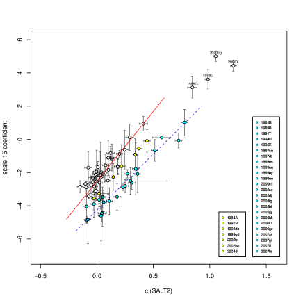
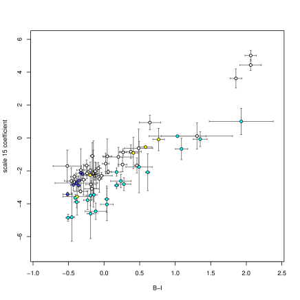
Figure 1: (a) Mean value of the wavelet coefficient from the largest scale for different spectra of nearby SNe Ia. The solid line corresponds to the best fit to “normal” SN data, while the dashed line describes the other SN class (see text for details). (b) Same as in (a), but using a long-baseline $B-I$ colour instead of the SALT2 $c$ parameter. Seven normal SNe that suffer negligible host extinction are identified as crossed symbols.

The robust regression fit in Fig. 1 reads $c\textrm{(SALT2)}=(0.406\pm 0.025)+(0.125\pm 0.009)\times\textrm{wltcoeff}_{\textrm{15}}$, with the standard deviation of fit $\hat{\sigma}=0.25$, computed as the median absolute deviation of the residuals divided by the constant $0.6745$. In order to reduce large data scatter, two perceivably distinctive SN trends are identified, represented by solid and dashed lines in Fig. 1:

$$c_{\textrm{(SALT2)}}=(0.300\pm 0.025)+(0.112\pm 0.012)\times\textrm{wltcoeff}_{\textrm{15}}$$ (1)

and

$$c_{\textrm{(SALT2)}}=(0.632\pm 0.026)+(0.149\pm 0.008)\times\textrm{wltcoeff}_{\textrm{15}}$$ (2)

respectively, with the robust measures of spread equal to 0.09, i.e. 0.11. Similarly, in Fig. 1, the scale 15 coefficient is well correlated with a long-baseline $B-I$ colour at $B$-band maximum corrected for Galactic reddening assuming $E(B-I)=2.35E(B-V)$. To calculate the uncertainty of the $(B-I)$ values, the photometric errors with the uncertainties due to the fitting procedure are combined.

A trend described by solid line in Fig. 1 is referred to as “normal” SNe. On the other hand, the earlier mentioned SN 2003fg is identified as a member of SN subclass (represented by dashed line), that includes objects whose colour appears to be redder than the typical SN Ia, according to the fits from Eqns. 1 and 2. Looking closely to the members of this SN group, represented by filled circles, there is some doubt whether these differences reflect the different explosion scenario or distinct progenitor channels, whether it can be attributed to the existence of (overdense) shell-structure in or around the SN ejecta, the interaction with the circumstellar material, massive progenitors, or finally, to different viewing angles of asymmetric envelopes, as will be discussed in subsequent section.

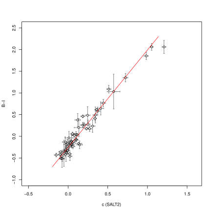
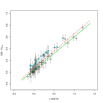
Figure 2: (a) $B-I$ vs the SALT2 $c$ parameter. (b) Estimated host galaxy reddening as a function of the SALT2 colour. Again, the filled circles correspond to those in Fig. 1. The best fit lines for all/normal SNe are shown as dashed/solid lines.

Indeed, Blondin et al. 2006 found that spectrum of SN 2003fg matches best with the spectrum of SN 1989B at $t=+3.5$ days (with constraints on epoch or redshift), an object also identified to belong to the same group. Howell et al. 2006 and Hillebrandt et al. 2007 debate between the possible explosion scenarios for SN 2003fg: a super-Chandrasekhar-mass progenitor explosion or the asymmetric explosion of a Chandrasekhar-mass ($M_{\textrm{Ch}}$) white dwarf? Something similar can be said for overluminous SN 2007if (Scalzo et al. 2010) and for SN 2006gz (Hicken et al. 2007), both with progenitor mass larger than $M_{\textrm{Ch}}$ and both surrounded by an envelope of unburned carbon/oxygen. Interestingly, SN 2009dc (Yamanaka et al. 2009), another SN with a massive progenitor, seems to be closer to normal SNe Ia in Fig. 1. Recently Silverman et al. 2011 published 9 spectra of this SN that cover the epochs from -7 days to +281 days and extend to $3500\;\textrm{\AA}$. An additional check for classification of this object on the spectrum at -7 days shows that the scale 15 coefficient for SN 2009dc is roughly $-4\pm 1$, therefore this SN belongs to the second group, as was expected. SNe Ia found to deviate from the main SN trend in Fig. 1, whose colours are described by Eqn. 2, may show significant discrepancy when a single parametrisation is applied, like the Phillips relation (Phillips 1993) that relates a light-curve width to peak luminosity, due to intrinsically different explosions. Also, as noted in Wang 2005, the circumstellar dust or a surrounding gaseous envelope may substantially affect the extinction properties compared to the interstellar dust. In other words, it is not wise to calibrate these SNe as standard candles; their reddenings will be more likely overestimated, which further implies that these objects are overcorrected to a higher luminosity, that could bias the cosmological results. Moreover, a certain number of SNe fall within the rough range $-0.1<c<0.1$. Interestingly, imposing this cut-off criterion in Fig. 1, the correlation between scale 15 coefficient and colour appears to be weak and the existence of distinct SN groups is no longer maintained. Nevertheless, one could select a subset of “more standardisable” SNe Ia based on the value of the largest wavelet scale coefficient.

3.1 Intrinsic SN colour and host galaxy reddening

As previously seen in Fig. 1, the scale 15 coefficient is correlated with both the SALT2 colour and long-baseline $B-I$ colour in a quite similar manner. Moreover, a strong relationship between these latter two is shown in Fig. 2. The best fit line corresponds to:

$$c_{\textrm{(SALT2)}}=(0.114\pm 0.007)+(0.445\pm 0.012)\times(B-I).$$ (3)

In Fig. 1 several SNe, namely 1990O, 1992A, 1994D, 1996X, 1998aq, 1999aw and 2000dk, that are thought to suffer negligible extinction in their host galaxies (as compiled from the literature, ${A_{V}}_{\textrm{host}}\lesssim 0.04$) are shown as crossed open circles. Putting all of these together,

$$(B-I)_{\textrm{max}}-E(B-I)_{\textrm{MW}}=(B-I)_{\textrm{max}}^{\textrm{int}}+E(B-I)_{\textrm{host}},$$ (4)

one expects that their colours corrected for Galactic extinction, $(B-I)_{\textrm{max}}^{\textrm{MW}_{\textrm{corr}}}$, are equal to the unreddened intrinsic colours at maximum, $(B-I)_{\textrm{max}}^{\textrm{int}}$. The best fit that provides the intrinsic $(B-I)$ colour relation for normal SNe is given by:

$$(B-I)_{\textrm{max}}^{\textrm{int}}=(0.013\pm 0.079)+(0.148\pm 0.029)\times\textrm{wltcoeff}_{\textrm{15}}.$$ (5)

The extinction affects colour estimation and is a source of systematic uncertainty. The SALT2 light-curve fitter is not meant to be able to disentangle the potential extinction by dust in the host galaxies from intrinsic colour variation. In the case of nearby SNe the SALT2 colour law should be consistent with observed law for extinction by dust in the Milky Way (extinction law by Cardelli, Clayton & Mathis 1989), but SN data point to a different colour-luminosity relation (see e.g. Astier et al. 2006). It is interesting to note that in the case of SNe 1999aa and 1997cn, two SNe that belong to other SN subsample discussed above and that do not suffer strong host galaxy extinction ($A_{V}=0.025\pm 0.020$, i.e. $0.025\pm 0.021$ respectively, according to the MLCS2k2 fits in Hicken et al. 2009), the relation given by Eqn. 5 is clearly unsatisfactory. Nevertheless, this is in agreement with findings in Wang et al. 2009, who reported two SN subsamples that favour different reddening laws. A possible explanation for this might be the existence of two SN populations with different intrinsic colours.

Furthermore, expression in Eqn. 4 and the obtained fits allow us to estimate the host galaxy reddening, implicitly assuming that $E(B-I)=2.35E(B-V)$. Adopting Eqn. 5 as the intrinsic colour relation for (all) SNe, the value of $E(B-V)_{\textrm{host}}$ can be directly obtained substituting expressions in Eqns. 3 and 5 in Eqn. 4:

$$E(B-V)_{\textrm{host}}=(0.069\pm 0.009)+(0.584\pm 0.028)\times c_{\textrm{(SALT2)}},$$ (6)

including all SNe in the fit (shown as dashed line in Fig. 2). On the other hand, excluding SNe that do not exhibit same properties as “normal” SNe (represented by filled symbols in Fig. 2) from the fit and keeping only them in the second case, one gets:

$$E(B-V)_{\textrm{host}}=(0.035\pm 0.006)+(0.569\pm 0.018)\times c_{\textrm{(SALT2)}},$$

i.e.

$$E(B-V)_{\textrm{host}}=(0.151\pm 0.007)+(0.553\pm 0.023)\times c_{\textrm{(SALT2)}},$$

respectively.

Again, there is a significant difference ($\sim$0.12 mag) in the reddening estimates between these two subsamples, implying that the two SN groups favour different reddening laws. However, this discrepancy may be due to assumption of the single intrinsic colour relation. Accounting for different intrinsic colour relations for the two SN subsamples may be a possible explanation for this. The main weakness of this analysis is the very limited number of normal SNe that enter the fit in Eqn. 5, also the lack of SN data that suffer no (or negligible) host extinction from other subsample that could provide an analogous intrinsic relation for intrinsically redder SNe.

3.2 High-$z$ sample

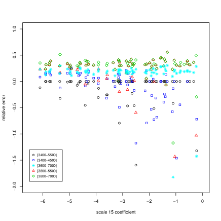
Figure 3: Comparison between wavelet coefficients at scale 15 calculated on the high-$z$ SNLS3 spectra for different wavelength intervals. The reference interval is $3400-7000\;\textrm{\AA}$.

An important question that needs to be asked is whether high-$z$ SNe follow the same correlations as those in the previous subsection. As an illustration, from the available set of high-$z$ spectra from SuperNova Legacy Survey 3-year sample (SNLS3), published in Balland et al. 2009, the wavelet analysis is applied to 94 SNe. Fig. 3 shows that the coefficient from the largest scale in the DTWT, measured on the high-$z$ sample, is relatively stable to changes in upper wavelength limit, probably because the majority of high-$z$ spectra do not reach $7000\;\textrm{\AA}$. Probing different wavelength intervals and identifying outliers, we find a high degree of agreement when comparing them. However, the wavelet coefficient at largest scale increases if the lower range limit shifts towards larger wavelengths compared to the reference one of $3400\;\textrm{\AA}$, which might be an important issue when studying nearby SNe.

3.3 Stability of the largest wavelet coefficient

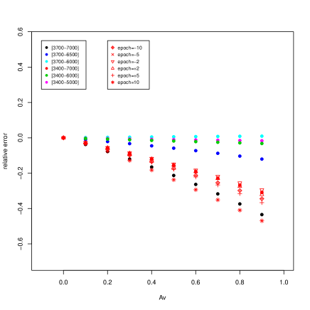
Figure 4: Comparison between wavelet coefficients associated with the largest scale calculated on the SALT2 spectral templates for different epochs and wavelength intervals after application of some amounts of reddening.

The results in Fig. 3 are compatible with tests based on measurements on the SALT2 spectral templates, as illustrated in Fig. 4. The wavelet coefficient from the coarsest scale is tested both for stability on chosen wavelength interval and epoch relative to $B$-band maximum. Although the dispersion seen when comparing different measurements can be up to 50 per cent near maximum, the coefficient value is relatively invariant across epoch over the range $[-10,+10]$ days. Furthermore, to include the dust effects, the spectral templates in the different wavelength intervals were reddened using the Milky Way (MW)-like extinction curve (Cardelli, Clayton & Mathis 1989) for different values of $R_{V}$ and $E(B-V)$. It has been shown that the effect of reddening does not strongly affect the equivalent width of a spectral feature, especially if it is narrow (e.g. Bronder et al. 2008; Arsenijevic et al. 2008). Similarly, despite the overall spectrum is somewhat warped, the relative error between different cases becomes significant mainly for large extinctions (Fig. 4). Furthermore, it can be seen that the dependence of the largest scale wavelet coefficient on extinction effects may be adjusted using specific wavelength intervals in the wavelet decomposition.

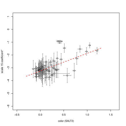
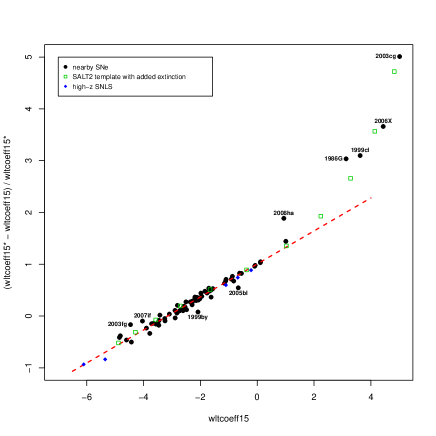
Figure 5: (a) Wavelet coefficient from the largest scale measured on the wavelet interval $[4000-6000\;\textrm{\AA}]$ versus SALT2 colour. (b) Comparison between the coefficients for different wavelength intervals. A linear fit (dashed line) can be used to test SNe Ia for anomalous extinction and/or peculiarity.

To test the effects of reddening, a subset of the “normal” SNe Ia was randomly chosen and some amount of reddening was applied to them. Indeed, after obtaining new coefficients from the fits, the differences are sufficiently large that may indicate the existence of two populations of SNe. However, as we have seen in Fig. 4, using the right wavelength interval, these differences can be controlled, i.e. minimised. For instance, choosing the intervals such as $[3700-6000\;\textrm{\AA}]$ or $[4000-6000\;\textrm{\AA}]$, the maximum relative error reduces to a few per cent, even for large extinction values that have been added.

The previously described method was performed on the same SN spectra, using the interval $[4000-6000\;\textrm{\AA}]$ (see Fig. 5). This choice guarantees the stability of the calculated values of the wavelet coefficient to the reddening uncertainties or instrumental distortions.

A robust regression analysis was performed to determine the best fit to the data in Fig. 5:

$$c_{\textrm{(SALT2)}}=(2.36\pm 0.12)+(0.73\pm 0.04)\times\textrm{wltcoeff}_{\textrm{15}}^{*},$$ (7)

where the asterisk denotes the coefficient obtained in the interval $[4000-6000\;\textrm{\AA}]$.

Moreover, in Fig. 5 it is demonstrated how to perform a test that identifies SNe Ia with anomalous extinction or strong peculiarity. For instance, apart from four outliers in Fig. 1 (SNe 1986G, 1999cl, 2003cg and 2006X), peculiar supernova 2008ha (extremely faint, 2002cx-like SN) strongly deviates from the main trend despite negligible host galaxy extinction reported in Foley et al. 2009. A few high-$z$ SNLS SNe whose spectra cover wavelengths up to 6700 Å are added to the plot (given as filled diamonds) showing an excellent agreement with nearby SNe.

Finally, different amounts ($0<A_{V}<4$, with the step $\Delta A_{V}=0.4$) of the MW-like extinction are applied to the SALT2 spectral template at maximum and obtained coefficients are plotted in Fig. 5. The data points follow the usual SN trend, even for the extinctions as large as 2.5 mags. Nevertheless, the figure clearly shows the two regimes, a linear ($A_{V}<2.5$), while there is an increase to the non-linear regime for heavily obscured SNe with $A_{V}>2.5$. In addition, strongly extinguished SNe such as 1999cl, 2003cg and 2006X, are consistent with this higher power law. After testing different extinction laws, we conclude that there is degeneracy between different models in the linear region; the differences mainly occur at higher values of extinction, i.e in the non-linear regime. The dependence of this combination of wavelet coefficients shown in Fig. 5 can be certainly used to estimate the amount of extinction towards an individual supernova.

4 Discussion

We are driven by need to grasp whether the existence of spectroscopic dichotomy, or even a quadrotomy, recently discussed in Wang et al. 2009 and Branch, Dang & Baron 2009 respectively, implies either different extinction laws or different colour evolution. As suggested in Wang 2005; Goobar 2008, the interaction between the SN ejecta and the surrounding circumstellar shell with normal dust grains could explain the reported values of $R_{V}$ that are lower than the standard Galactic value of $3.1$. Furthermore, the SN spectra at early epochs are sensitive to the material in which the supernovae are embedded. Emitted SN light is therefore reflected by the surrounding dust clouds and reaches the observer at different times from different directions, as a result of the interaction that, generally speaking, depends on the location of the dust clouds, the density distribution of dust grains and/or the scattering properties of dust. Moreover, if the dust optical depth is low, one may assume a simple scattering scenario in which a photon escapes after scattering off dust particle. It becomes more difficult when thick dust shells and complex dust mixtures are considered, where multiple scatterings usually occur. Following Patat et al. 2007; Blondin et al. 2009, the presence of high-velocity features in spectra and time-variable Na ID absorption feature is good signature of influence of effects of circumstellar dust on the SN luminosity (typical examples are SNe 1999cl and 2006X). Besides, SN 2006X suffers significant reddening from the interstellar medium (Wang et al. 2008). However, not all highly reddened SNe Ia display variable Na ID features: SN 2003cg is heavily extinguished, very large Na ID equivalent width values (compared to other SNe) were measured for this SN, but the feature remains constant over time. The previously described scenario can cause an effect of the light echo around supernova, already seen, for instance, for SNe 1991T, 1995E, 1998bu, 2000cx, 2002ic, 2006X (Patat et al. 2007; Wang 2005). Similarly, the dust shells that surround (not necessarily highly extinguished) SNe Ia, are reported also for SN 2005gj, then 2007gi and 2007le. Indeed, all of these mentioned SNe are leaned towards the second fit in Fig. 1. This latter supernova, recently discovered SN 2007le (Simon et al. 2009), however, exhibits variable Na ID line but, curiously, is low extinguished, which further reflects its intrinsic property. In addition, Yuan et al. 2010 consider the interaction between the ejecta and the circumstellar material as an alternative manner for a supernova to generate extra luminosity, rather than any intrinsic property of the SN. Moreover, a supernova with extremely low luminosity, SN 2008ha (Foley et al. 2009), that is spectroscopically similar to peculiar SN 2002cx (Li et al. 2003), is in an excellent agreement with the red solid line in Fig. 1, although it is an outlier in Fig. 5. As noted in Li et al. 2003, SN 2002cx is a link between the extremes of peculiar SNe Ia. Indeed, this SN exhibits the 1991T-like premaximum spectra, but is subluminous, such as 1991bg-like SNe. Nevertheless, the wavelet coefficient from the largest scale reflects spectroscopic diversity of SNe Ia, pointing to a common property of this trend, regardless if an SN has already been classified as 1991T-, 1991bg-, 1999aa- or 2000cx-like event.

On the other hand, SNe such as 1999ee and 1989B are also found to show affinity for this group. These SNe exhibit a plateau in the photospheric velocity near $B$-maximum, while normally, a standard SN Ia has very steep velocity change from early phases towards maximum. This plateau tendency (more precisely, a period of slowly declining velocities) coincides with the photosphere receding through the overdense shell (Scalzo et al. 2010; Quimby, Höflich & Wheeler 2007). The similar has been noticed for SNe 1991T, 1999aa, 2000cx (see e.g. Benetti et al. 2005; Quimby, Höflich & Wheeler 2007), all of them having redder $(B-V)$ colour at maximum. Quimby, Höflich & Wheeler 2007 report nearly the same velocity evolution of the Si II line for SN 2005hj, but the available spectra for this SN do not cover wavelengths $\lambda\lesssim 3885$, therefore the value of wavelet coefficient of interest is most likely overestimated (see Figs. 3 and 4).

Another intriguing result is that the high velocity gradient (HVG, Benetti et al. 2005) SNe, namely SNe 1998de, 1999gd, 2002bo, 1984A, 2002bf, 1991M and 2004dt, given as light filled circles in Fig. 1 and ordered by decreasing colour, are found to be transitional objects, linking the two main SN trends. A possible interpretation of this observed continuity between the groups could be accounted as an effect of mixed extinction that these SNe suffer, partly caused by circumstellar, but could also be due to interstellar dust. However, another HVG SN 1981B is found in the CSM group. In addition, a few more SNe are identified very close to these HVG SNe in direction towards normal SNe, namely: 1998bp, 1998bu, 1999aw, 2000cf, 2001V, 2001el. Again, these latter are characterised by whether the higher polarisation (e.g. SN 2001el), or close resemblance to 1999aa-like or under(over)luminous SNe. On the other hand, it has been found recently (Maeda et al. 2010) that HVG and LVG SNe, despite the divergence in photospheric velocity, do not have intrinsic differences. The diversity between these two supernova groups appears as a consequence of different viewing angle from which an SN is observed. In other words, if one obtains a big enough SN sample, these differences will average out and this issue will be of no concern for the cosmological use of SNe Ia. However, the redder SN population that satisfies relation in Eqn. 2, must be treated with caution because our findings point to different intrinsic colour relations for the two SN subsamples.

Given the previous discussion, our analysis suggests the existence of a distinct class of SNe that is more likely governed by different physical mechanism, i.e. considered to have a different progenitor system and/or explosion mechanism than standard SNe Ia. Interestingly, SNe that support both single- (e.g. SN 2005gj, Aldering et al. 2006; Prieto et al. 2007) and double-degenerate (e.g. SN 2003fg and/or SN 2006gz, with detected envelope of unburned carbon) scenario are found in the same group. Nevertheless, if one suspects that the circumstellar dust is present around an SN Ia, it is not advisable to assume a standard interstellar extinction law, but rather should be studied it by implementing a radiative transfer code. The effective extinction is supposed to be generally smaller when the scattering effects are included into consideration, since the contribution of scattered photons makes that the total flux increases. The light that has been scattered off the circumstellar dust cloud aims to lower the effective total to selective extinction ratio in the optical range, completely opposite from the effect it causes in the UV (see e.g. Wang 2005). A possibility that SN colours correlate with intrinsic brightness of SNe Ia in such a way that this correlation resembles reddening by dust is not rejected as well, as has been indirectly shown in relations from Fig. 1 and Eqn. 5. It is also implicitly assumed throughout that the SALT2 colour estimation is essentially perfect, despite the fact that its training procedure is based on a sample of SNe Ia.

Summing up, around 30 per cent of nearby SNe in our sample are found to depart from the main SN trend in Fig. 1. Assuming that the similar fraction of high-$z$ population follows this tendency, a contamination of cosmological sample by these objects could be significant. Recall that Wang et al. 2009 recently proposed two different $R_{V}$ corrections for normal and high velocity (HV) samples, which notably improved the accuracy of distance measurements. Furthermore, the same authors showed that the HV SNe prefer a lower value of the extinction ratio $R_{V}$. On the other hand, our measurements on the spectral template show that the largest wavelet scale coefficient is fairly stable under different extinction laws, which suggests that this observed discrepancy has an intrinsic character. Indeed, the two SN subsamples may have the same host galaxy reddening law if the intrinsic colour relations were properly accounted for.

In addition, even the highly-reddened SNe are consistent with the MW-like dust extinction behaviour in Fig. 5. Tests with different $R_{V}$ values than the canonical Galactic value of $3.1$ also suggest that anomalous behaviour is most likely due to high reddening. The extinction law for the circumstellar dust from Goobar 2008 is also tested and it appears very much like the curve with the MW extinction in the linear part, while it is steeper in the non-linear regime, although for significantly smaller values of extinction (for example, for a fixed value of $R_{V}=1.8$, a CS curve that fits SN 2003cg measurements has $A_{V}\sim 2.2$, compared to the MW curve with $A_{V}\sim 2.5$). In order to include a more significant high-$z$ SN sample into the analysis (compared with those few SNe that are found in Fig. 5), another pair of the wavelength intervals should be studied, ones that correspond better to the rest-frame coverage of high-$z$ SN spectra, for example between $3000<\lambda<5000\;\textrm{\AA}$.

Wavelet scales that are directly responsible for spectral features are free of any intrinsic color information in the input spectra, which justifies a recent attempt to quantify SN spectral features that was done by Wagers, Wang & Asztalos 2010. They found correlations between various combinations of spectral features with stretch. This is surely an important question that should be further explored.

5 Conclusions

The presented technique is used to test SN diversity, i.e. how significantly the explosion of a supernova differs from widely accepted SN Ia progenitor scenarios, which may further lead to different intrinsic colour. For this purpose, the wavelet transform is used to decompose SN spectra into different scales. The largest scale coefficient is found to correlate with the SALT2 colour parameter and long-baseline $B-I$ colour corrected for Galactic reddening. Apart from the main trend with normal SNe Ia, another grouping is distinguished; its members have intrinsically redder colours when compared to the normal ones and are recognised for various characteristics such as the observed light echo around SN, or in addition, a signature of interaction with circumstellar material, and/or the existence of shell-structure in or surrounding the SN ejecta. Moreover, a few candidates of super-Chandrasekhar mass SNe show affinity for this group. However, the questions on details on circumstellar dust shell (or inner overdense shell), such as its mass or its geometry, are not tackled in this work.

This study has shown that SALT2 colour parameter can be disentangled into intrinsic SN colour and the reddening due to dust extinction in the host galaxy. However, with the lack of SNe from intrinsically redder subsample that suffer negligible host galaxy extinction, the expressions for intrinsic colour and host galaxy reddening have been found only for normal SNe. In order to prevent the overcorrected luminosities, mentioned redder SNe should be identified and calibrated in a different manner before being included in the cosmology fits.

The wavelet coefficients that were measured on certain wavelength intervals are invariant to additional amounts of extinction that were applied to the spectra. A combination of two largest scale coefficients from different intervals can be further used to distinguish objects that exhibit strong peculiarities and/or to estimate the extinction value.

The method for additional SN sorting presented in this paper is applicable regardless either of the type of wavelets used in the analysis or of the number of scales in the wavelet decomposition. Nevertheless, there is certainly room for improvement, especially in estimating the largest wavelet scale coefficient when the available spectra lack the full wavelength coverage. Similarly, an additional correction could be applied to account for spectral epochs different from the reference one at maximum light. The implementation of the presented analysis by incorporating larger and homogeneous spectral and photometric data will permit a deeper insight into the extinction corrections, also the variety of the SN progenitor environments and explosion models and will be the topic of future work.

Acknowledgements

We are grateful to R. Kirshner and S. Blondin for generously allowing us to use the CfA spectra of SN 2007af and SN 1995E before publication, also for useful discussion. We thank P. Nugent for the valuable comments that helped us to improve the manuscript. V. Arsenijevic acknowledges support from FCT under grant no. SFRH/BPD/47498/2008. This work made use of the SUSPECT (http://bruford.nhn.ou.edu/~suspect/index1.html) and the CfA (http://www.cfa.harvard.edu/supernova/SNarchive.html) SN archives.

Table 1: List of SNe Ia used in our study.

SN name	Redshift	$x_{1}$	$c$	$\chi^{2}/\textrm{dof}$	$\textrm{wltcoeff}_{\textrm{15}}$	$\textrm{wltcoeff}_{\textrm{15}}^{*}$	Refs
1981B	0.0072	$-0.472\pm 0.138$	$0.048\pm 0.038$	1.032	$-4.428\pm 0.800$	$-2.948\pm 0.624$	1
1984A	-0.0009	$0.051\pm 0.050$	$0.218\pm 0.032$	26.152	$-1.622\pm 1.304$	$-2.555\pm 0.147$	4
1986G	0.0018	$-2.226\pm 0.142$	$0.845\pm 0.042$	1.378	$3.128\pm 0.639$	$-1.536\pm 0.256$	1
1989B	0.0024	$-0.913\pm 0.105$	$0.343\pm 0.028$	0.713	$-1.767\pm 1.565$	$-3.181\pm 0.589$	1
1990N	0.0034	$0.996\pm 0.094$	$0.008\pm 0.025$	2.025	$-1.680\pm 0.349$	$-3.242\pm 0.692$	1
1990O	0.0307	$0.450\pm 0.191$	$-0.053\pm 0.032$	0.296	$-2.740\pm 0.500$	$-3.037\pm 0.058$	10
1991M	0.0072	$-1.082\pm 0.239$	$0.018\pm 0.089$	0.569	$-3.254\pm 0.800$	$-3.103\pm 0.596$	1
1991T	0.0058	$1.410\pm 0.087$	$0.112\pm 0.025$	2.100	$-3.718\pm 0.800$	$-3.235\pm 0.760$	1
1991bg	0.0030	$-1.377\pm 0.057$	$0.290\pm 0.034$	31.701	$0.118\pm 0.800$	$-2.466\pm 0.614$	1
1992A	0.0061	$-1.632\pm 0.051$	$-0.013\pm 0.024$	1.368	$-2.115\pm 0.326$	$-3.136\pm 0.514$	1
1994D	0.0015	$-1.741\pm 0.045$	$-0.095\pm 0.024$	1.258	$-2.893\pm 0.346$	$-3.244\pm 0.381$	1
1994U	0.0048	$0.000\pm 7.465$	$0.297\pm 0.323$	3.341	$-2.507\pm 0.800$	$-3.447\pm 0.660$	14, 15
1995E	0.0118	$-0.488\pm 0.122$	$0.723\pm 0.030$	0.542	$-0.072\pm 0.443$	$-3.223\pm 0.576$	15, this work
1996X	0.0068	$-1.011\pm 0.095$	$-0.039\pm 0.028$	0.200	$-2.582\pm 0.277$	$-3.179\pm 0.529$	1
1997br	0.0070	$0.369\pm 0.098$	$0.200\pm 0.027$	7.670	$-0.873\pm 0.206$	$-3.736\pm 0.661$	1
1997cn	0.0162	$-0.550\pm 0.116$	$0.777\pm 0.030$	23.903	$1.007\pm 0.800$	$-2.274\pm 0.467$	1
1997do	0.0101	$0.220\pm 0.155$	$0.070\pm 0.026$	2.567	$-2.020\pm 0.551$	$-3.024\pm 0.497$	2
1997dt	0.0073	$-0.141\pm 0.290$	$0.574\pm 0.080$	0.346	$0.111\pm 0.066$	$-3.602\pm 0.558$	2
1998V	0.0176	$-0.333\pm 0.087$	$-0.004\pm 0.026$	1.734	$-1.951\pm 1.296$	$-3.149\pm 0.673$	2
1998aq	0.0037	$-0.353\pm 0.036$	$-0.150\pm 0.025$	1.398	$-2.848\pm 0.353$	$-3.088\pm 0.672$	1, 2
1998bp	0.0104	$-2.440\pm 0.169$	$0.184\pm 0.031$	1.108	$-1.618\pm 0.435$	$-3.246\pm 0.644$	2
1998bu	0.0030	$-0.344\pm 0.029$	$0.185\pm 0.027$	3.116	$-1.671\pm 0.458$	$-3.266\pm 0.674$	1, 2
1998de	0.0167	$-3.061\pm 0.133$	$0.443\pm 0.029$	2.988	$-0.091\pm 0.684$	$-2.341\pm 0.465$	2
1998dh	0.0089	$-0.692\pm 0.106$	$0.055\pm 0.027$	1.346	$-2.062\pm 0.123$	$-3.169\pm 0.346$	2
1998dm	0.0066	$0.596\pm 0.251$	$0.245\pm 0.031$	0.965	$-0.621\pm 1.160$	$-3.585\pm 0.427$	2
1998ec	0.0199	$-0.188\pm 0.323$	$0.134\pm 0.057$	0.435	$-1.153\pm 0.582$	$-3.121\pm 0.652$	2
1998eg	0.0248	$-0.700\pm 0.316$	$-0.009\pm 0.028$	0.370	$-2.151\pm 0.329$	$-3.068\pm 0.631$	2
1998es	0.0106	$1.011\pm 0.119$	$0.036\pm 0.025$	0.553	$-4.600\pm 1.523$	$-3.144\pm 0.674$	2
1999X	0.0252	$-0.529\pm 0.498$	$0.010\pm 0.050$	0.271	$-2.293\pm 0.191$	$-3.096\pm 0.524$	2
1999aa	0.0144	$1.170\pm 0.093$	$-0.079\pm 0.025$	0.803	$-4.817\pm 1.470$	$-3.486\pm 0.566$	1, 2
1999ac	0.0095	$0.206\pm 0.064$	$0.029\pm 0.024$	3.220	$-2.129\pm 1.388$	$-3.329\pm 0.691$	1, 2
1999aw	0.0380	$2.339\pm 0.166$	$-0.075\pm 0.029$	1.649	$-3.425\pm 0.132$	$-3.484\pm 0.033$	1,2
1999by	0.0021	$-1.444\pm 0.063$	$0.360\pm 0.025$	17.604	$-2.085\pm 1.116$	$-2.261\pm 0.497$	1, 2
1999cc	0.0313	$-1.582\pm 0.199$	$-0.025\pm 0.031$	0.220	$-2.826\pm 0.224$	$-2.999\pm 0.627$	2
1999cl	0.0076	$-0.753\pm 0.167$	$0.984\pm 0.027$	1.581	$3.622\pm 0.582$	$-1.726\pm 0.303$	2
1999dq	0.0143	$0.826\pm 0.062$	$0.033\pm 0.025$	0.867	$-2.193\pm 2.014$	$-3.457\pm 0.682$	2
1999ee	0.0113	$0.722\pm 0.039$	$0.231\pm 0.023$	0.690	$-2.888\pm 0.191$	$-2.785\pm 0.576$	1
1999ej	0.0137	$-1.400\pm 0.217$	$-0.037\pm 0.038$	0.490	$-2.290\pm 0.272$	$-3.206\pm 0.493$	2
1999gd	0.0185	$-1.082\pm 0.126$	$0.372\pm 0.029$	1.829	$-0.555\pm 0.070$	$-3.134\pm 0.629$	2
1999gh	0.0077	$-2.329\pm 0.152$	$0.120\pm 0.034$	0.381	$-0.828\pm 0.410$	$-2.554\pm 0.478$	2
1999gp	0.0267	$1.749\pm 0.083$	$-0.004\pm 0.018$	1.082	$-2.539\pm 0.936$	$-3.068\pm 0.619$	2
2000E	0.0047	$0.476\pm 0.062$	$0.102\pm 0.024$	3.382	$-1.839\pm 0.348$	$-3.528\pm 0.668$	1
2000cf	0.0364	$-0.959\pm 0.210$	$-0.034\pm 0.029$	0.467	$-3.245\pm 0.101$	$-2.967\pm 0.392$	2
2000cn	0.0235	$-2.247\pm 0.209$	$0.077\pm 0.028$	0.652	$-1.562\pm 0.630$	$-3.311\pm 0.114$	2
2000cx	0.0079	$-1.001\pm 0.042$	$-0.088\pm 0.024$	5.622	$-4.849\pm 0.207$	$-3.430\pm 0.550$	1, 2
2000dk	0.0174	$-1.871\pm 0.144$	$-0.032\pm 0.027$	0.454	$-2.194\pm 0.265$	$-3.335\pm 0.439$	2
2000fa	0.0213	$0.554\pm 0.187$	$0.035\pm 0.029$	0.249	$-2.292\pm 0.771$	$-2.927\pm 0.637$	2
2001V	0.0160	$0.988\pm 0.094$	$-0.010\pm 0.020$	0.950	$-3.091\pm 0.675$	$-3.212\pm 0.607$	2
2001el	0.0039	$-0.245\pm 0.039$	$0.097\pm 0.024$	3.477	$-2.487\pm 0.826$	$-2.830\pm 0.050$	1
2002bf	0.0242	$-0.298\pm 0.145$	$0.144\pm 0.034$	1.087	$-2.268\pm 0.800$	$-3.170\pm 0.493$	1
2002bo	0.0042	$-0.471\pm 0.038$	$0.339\pm 0.018$	1.425	$-0.909\pm 0.951$	$-3.157\pm 0.615$	1
2002cx	0.0240	$0.351\pm 0.136$	$0.308\pm 0.031$	6.960	$-2.620\pm 0.400$	$-3.082\pm 0.565$	1
2002dj	0.0094	$0.028\pm 0.146$	$0.060\pm 0.025$	0.934	$-3.781\pm 0.568$	$-2.831\pm 0.631$	13
2002er	0.0086	$-0.764\pm 0.057$	$0.100\pm 0.024$	0.929	$-1.112\pm 1.054$	$-3.423\pm 0.620$	1
2003cg	0.0041	$-0.802\pm 0.039$	$1.053\pm 0.019$	4.988	$5.011\pm 0.312$	$-1.249\pm 0.204$	1
2003du	0.0064	$0.294\pm 0.039$	$-0.102\pm 0.017$	1.342	$-2.686\pm 0.187$	$-3.058\pm 0.437$	1
2003fg	0.2437	$1.134\pm 0.306$	$0.043\pm 0.030$	10.955	$-4.459\pm 0.500$	$-3.824\pm 0.638$	12
2004S	0.0091	$-0.217\pm 0.087$	$0.022\pm 0.026$	0.933	$-2.612\pm 0.800$	$-2.912\pm 0.481$	1
2004dt	0.0197	$-0.885\pm 0.048$	$-0.027\pm 0.024$	3.012	$-3.567\pm 1.113$	$-3.090\pm 0.594$	1, 3
2004eo	0.0157	$-1.044\pm 0.036$	$0.039\pm 0.024$	1.098	$-1.982\pm 0.136$	$-3.549\pm 0.155$	1
2005am	0.0079	$-2.034\pm 0.094$	$0.133\pm 0.040$	1.642	$-1.096\pm 0.800$	$-3.755\pm 0.593$	1
2005bl	0.0251	$-2.185\pm 0.100$	$0.513\pm 0.027$	7.728	$-0.667\pm 0.653$	$-1.465\pm 0.342$	11
2005cf	0.0065	$-0.134\pm 0.054$	$-0.034\pm 0.024$	1.119	$-2.356\pm 0.149$	$-3.235\pm 0.463$	1
2005gj	0.0593	$5.000\pm 0.015$	$0.178\pm 0.034$	9.610	$-3.464\pm 0.800$	$-2.941\pm 0.587$	19,20
2005hj	0.0580	$2.279\pm 0.408$	$-0.077\pm 0.032$	0.778	$-1.703\pm 0.967$	$-3.679\pm 0.094$	1
2005hk	0.0130	$0.044\pm 0.058$	$0.250\pm 0.027$	32.085	$-2.808\pm 0.390$	$-3.537\pm 0.670$	1
2006D	0.0097	$1.341\pm 0.044$	$0.019\pm 0.023$	1.288	$-3.645\pm 0.205$	$-3.200\pm 0.164$	16
2006X	0.0063	$-0.258\pm 0.040$	$1.209\pm 0.025$	2.411	$4.434\pm 0.326$	$-1.667\pm 0.253$	5,6
2006gz	0.0280	$2.228\pm 0.120$	$-0.027\pm 0.025$	1.018	$-3.898\pm 0.347$	$-3.161\pm 0.695$	1
2007af	0.0063	$-0.431\pm 0.059$	$0.052\pm 0.027$	0.545	$-3.455\pm 0.414$	$-3.185\pm 0.457$	7, this work
2007if	0.0731	$2.964\pm 0.198$	$-0.092\pm 0.030$	2.180	$-4.039\pm 0.994$	$-3.681\pm 0.598$	17,18
2007le	0.0055	$0.152\pm 0.054$	$0.270\pm 0.027$	1.127	$-2.073\pm 0.247$	$-2.997\pm 0.568$	8
2007gi	0.0053	$-1.260\pm 0.117$	$0.049\pm 0.029$	1.538	$-3.497\pm 0.621$	$-3.088\pm 0.585$	9
2008ha	0.0034	$-3.415\pm 0.353$	$0.411\pm 0.037$	1.620	$0.937\pm 0.440$	$-1.057\pm 0.253$	21
(1) Arsenijevic et al. 2008 and references therein; (2) Matheson et al. 2008; (3) Contreras et al. 2010; (4) Barbon et al. 1989; (5) Wang et al. 2008; (6) Yamanaka et al. 2009b; (7) Simon et al. 2007; (8) Simon et al. 2009; (9) Zhang et al. 2010; (10) Permutter et al. 1999; (11) Taubenberger et al. 2008; (12) Howell et al. 2006; (13) Pignata et al. 2008; (14) Gómez & López 1998; (15) Riess et al. 1998; (16) Thomas et al. 2007; (17) Scalzo et al. 2010; (18) Yuan et al. 2010; (19) Prieto et al. 2007; (20) Aldering et al. 2006; (21) Foley et al. 2009.

References

- Aldering et al. (2006) Aldering, G. et al. 2006, ApJ, 650, 510
- Arsenijevic et al. (2008) Arsenijevic, V. et al. 2008, A&A, 492, 535
- Astier et al. (2006) Astier, P. et al. 2006, A&A, 447, 31
- Balland et al. (2009) Balland, C. et al. 2009, A&A, 507, 85
- Bailey et al. (2009) Bailey, S. et al. 2009, A&A, 500, 17
- Barbon et al. (1989) Barbon, R. et al. 1989, A&A, 220, 83
- Benetti et al. (2005) Benetti, S. et al. 2005, ApJ, 623, 1010
- Blondin et al. (2009) Blondin, S. et al. 2009, ApJ, 693, 207
- Blondin et al. (2006) Blondin, S. et al. 2006, AJ, 131, 1648
- Branch, Dang & Baron (2009) Branch, D., Dang, L. C. & Baron, E. 2009, PASP, 121, 238
- Bronder et al. (2008) Bronder, J. et al. 2008, A&A, 477, 717
- Cardelli, Clayton & Mathis (1989) Cardelli, J. A., Clayton, G. C. & Mathis, J. S. 1989, ApJ, 345, 245
- Conley et al. (2008) Conley, A. et al. 2008, ApJ, 681, 482
- Contreras et al. (2010) Contreras, C. et al. 2010, AJ, 139, 519
- Foley et al. (2009) Foley, R. et al. 2009, AJ, 138, 376
- Gómez & López (1998) Gómez, G. & López, R. 1998, AJ, 115, 1096
- Goobar (2008) Goobar, A. 2008, ApJ, 686L, 103
- Guy et al. (2007) Guy, J. et al. 2007, A&A, 466, 11
- Hachinger, Mazzali & Benetti (2006) Hachinger, S., Mazzali, P. A. & Benetti, S. 2006, MNRAS, 370, 299
- Hicken et al. (2009) Hicken, M. et al. 2009, ApJ, 700 1097
- Hicken et al. (2007) Hicken, M. et al. 2007, ApJ, 669, L17
- Hillebrandt et al. (2007) Hillebrandt, W., Siml, S. A., & Röpke, F. K. 2007, A&A, 465, L17
- Howell et al. (2006) Howell, D. A. et al. 2006, Nature, 443, 309
- Jha, Riess & Kirshner (2007) Jha, S., Riess, A. G., Kirshner, R. P. 2007, ApJ, 659, 122
- Li et al. (2003) Li, W. et al. 2003, PASP, 115, 453
- Maeda et al. (2010) Maeda, K. et al. 2010, Nature, 466, 82
- Matheson et al. (2008) Matheson, T. et al. 2008, AJ, 135, 1598
- Mazzali et al. (2007) Mazzali, P. A. et al. 2007, Science, 315, 825
- Nugent et al. (1995) Nugent, P. et al. 1995, ApJ, 455, L147
- Patat et al. (2007) Patat, F. et al. 2007, Science, 317, 924
- Permutter et al. (1999) Perlmutter, S. et al. 1999, ApJ, 517, 565
- Phillips (1993) Phillips, M. M. 1993, ApJ, 413, 105
- Pignata et al. (2008) Pignata, G. et al. 2008, MNRAS, 388, 971
- Prieto et al. (2007) Prieto, J. L. et al. 2007, arXiv:astro-ph/0706.4088
- Quimby, Höflich & Wheeler (2007) Quimby, R., Höflich, P. & Wheeler, C. J. 2007, ApJ, 666, 1083
- Riess et al. (1998) Riess, A. G. et al. 1998, AJ, 116, 1009
- Scalzo et al. (2010) Scalzo, R. A et al. 2010, ApJ, 713, 1073
- Silverman et al. (2011) Silverman, J. M. et al. 2011, MNRAS, 410, 585
- Simon et al. (2009) Simon, J. D. et al. 2009, ApJ, 702, 1157
- Simon et al. (2007) Simon, J. D. et al. 2007, ApJ, 671, 25
- Tanaka et al. (2009) Tanaka, M. et al. 2009, ApJ, 714, 1209
- Taubenberger et al. (2008) Taubenberger, S. et al. 2008, MNRAS, 385, 75
- Thomas et al. (2007) Thomas, R. C. et al. 2007, ApJ, 654, 53
- Wagers, Wang & Asztalos (2010) Wagers, A., Wang, L. & Asztalos, S. 2010, ApJ, 711, 711
- Wang et al. (2009) Wang, X. et al. 2009, ApJ, 699, L139
- Wang et al. (2008) Wang, X. et al. 2008, ApJ, 675, 626
- Wang (2005) Wang, L. 2005, ApJ, 635, 33
- Yamanaka et al. (2009) Yamanaka, M. et al. 2009, ApJ, 707, 118
- Yamanaka et al. (2009b) Yamanaka, M. et al. 2009, PASJ, 61, 713
- Yuan et al. (2010) Yuan, F. et al. 2010, ApJ, 715, 1338
- Zhang et al. (2010) Zhang, T. et al. 2010, PASP, 122, 1