Abstract

We test a recent proposal to use approximate trivializing maps in a field theory to speed up Hybrid Monte Carlo simulations. Simulating the CP^N-1model, we find a small improvement with the leading order transformation, which is however compensated by the additional computational overhead. The scaling of the algorithm towards the continuum is not changed. In particular, the effect of the topological modes on the autocorrelation times is studied.

CERN-PH-TH/2011-023

1 Introduction

In the simulation of statistical models, many Monte Carlo methods experience a significant increase in effort when approaching a continuous phase transition of the theory. This phenomenon is called critical slowing down and depends strongly on the nature of the underlying theory and the algorithm used. For some models, algorithms have been found which completely eliminate this slowing down or even lead to a speed-up when the critical line is approached. A particular type of critical slowing down is associated with the topological modes of the theories. In QCD, e.g., the topological charge of the gauge configuration is known to be particularly problematic with both single link updates [1] and algorithms based on molecular dynamics [2].

Recently, a possible solution to the problem has been proposed [3], for which field transformations given by flow equations are introduced. Exactly integrating the flow equations, the theory becomes trivial and therefore also trivial to simulate. The problem is that the differential equations generating the flow are not exactly known, however, the first terms of a power series of the corresponding kernel can easily be constructed. At this point, it is unclear whether it is sufficient to just know the first order of the differential equations to sufficiently mitigate the problem. Also the accuracy to which the differential equations have to be integrated is unknown.

In this letter, we therefore put this proposal to a test. Since it should work for any field theory, we simulate the CP^N-1model for $N=10$ using the Hybrid Monte Carlo (HMC) algorithm [4], which is an integral part of the program laid out in Ref. [3]. We choose this model, because it shares some similarities with QCD like asymptotic freedom and confinement and, like in QCD, the topological modes show a much more severe critical slowing down than other observables [5]. Most importantly, the accuracy achievable in this two dimensional model is much higher than in QCD and the reduced cost also allows for a better mapping of the rather high dimensional parameter space of the problem.

In Sect. 2 we give the details of the model and how to set up the HMC algorithm for it. After that, we discuss the trivializing map and its construction to leading order in Sec. 3. Then we give the parameters of the simulation which enables us to put the approximate trivializing map to a test whose results we give in Sect. 4. In the definition of the action, the observables and as a point of reference for the main quantities, we follow the paper by Campostrini, Rossi and Vicari [6].

2 The CP^N-1model and Hybrid Monte Carlo

We immediately give the model on a square lattice with lattice spacing $a$ and sites $n=a(n_{1},n_{2})$, $n_{1}$ and $n_{2}$ integer numbers. The fields living on the sites are complex $N$ component unit vectors $z_{n}$ connected by U(1) link variables $\lambda_{n,\mu}$, which are represented by complex numbers on the unit circle. The action is then given by [7]

$$S[z,\lambda]=-N\beta\sum_{n}\sum_{\mu=1}^{2}\left(z_{n+\hat{\mu}}^{\dagger}z_{n}\lambda_{n,\mu}+z_{n}^{\dagger}z_{n+\hat{\mu}}\lambda_{n,\mu}^{*}-2\right)\;.$$ (1)

The gauge fields $\lambda_{n,\mu}$ can be integrated out analytically, thus this lattice action is expected to lie within the universality class of the CP^N-1model.

For the Hybrid Monte Carlo algorithm as well as for the field transformation we will need derivatives with respect to the field degrees of freedom. Therefore it is convenient to treat the fields as $real$ $2N$ component fields $x_{n}$, which live on the unit sphere in $\mathbb{R}^{2N}$

$$x_{n,2i}=\mathrm{Re}{(z_{n,i})}\;,\;\;x_{n,2i+1}=\mathrm{Im}{(z_{n,i})}\;\;\;,\;i=0,\dots,N-1\;.$$ (2)

In the following, we will make use of either $z$ or $x$, such that each formula appears in its most simple form.

The $U(1)$ fields $\lambda$ are naturally parametrized by the angle $\phi\in[0,2\pi)$ with $\lambda=e^{i\phi}$. Its action on the vectors $x$ is then given by SO(2) $2N\times 2N$ matrices $\Lambda_{n,\mu}(\phi)$, which are zero everywhere but on the diagonal $2\times 2$ blocks

$$\begin{pmatrix}\Lambda_{2i,2i}&\Lambda_{2i,2i+1}\\ \Lambda_{2i+1,2i}&\Lambda_{2i+1,2i+1}\end{pmatrix}=\begin{pmatrix}\cos\phi&-\sin\phi\\ \sin\phi&\cos\phi\end{pmatrix}\;\;,\;i=0,\dots,N-1\;.$$

With these definitions, we can write the action as function of real variables only

$$S[x,\phi]=-N\beta\sum_{n}\left(x_{n}^{T}J_{n}-4\right)\;,$$ (3)

where we introduced the “spin sum” of gauge-transported nearest neighbors

$$J_{n} = \sum_{\mu=\pm 1}^{\pm 2}\Lambda_{n,\mu}^{T}x_{n+\hat{\mu}}\;,\;\;\;\text{with}\;\;\Lambda_{n,-\mu}:=\Lambda_{n-\hat{\mu},\mu}^{T}\;.$$ (4)

The partition function can then be easily written by embedding the unit vectors $x_{n}$ into $\mathbb{R}^{2N}$.

2.1 Observables

We will focus our study on a few, central observables. Mainly the energy density $E=S/(N\beta V)$, the magnetic susceptibility $\chi_{M}$ and the correlation length $\xi_{G}$. The latter two are constructed from the two point function in momentum space

$$\widetilde{G}_{P}({k})=\frac{1}{V}\sum_{n,m}\langle\mathrm{tr}P_{n}P_{m}\rangle_{\mathrm{conn}}\exp\left(\frac{2\pi i}{L}({n-m})\cdot{k}\right)$$ (5)

with $P_{n}=z_{n}z_{n}^{\dagger}$. Using these definitions, the two remaining observables are then

$$\chi_{M}=\widetilde{G}_{P}(0,0)\ ;\qquad\xi_{G}^{2}=\frac{1}{4\sin^{2}\frac{\pi}{L}}\left(\frac{\widetilde{G}_{P}(0,0)}{\widetilde{G}_{P}(0,1)}-1\right)\ .$$ (6)

The topological charge density $q_{n}$ is given by the sum over the angles between the spins around a plaquette

$$q_{n}=\frac{1}{4\pi}\epsilon_{\mu\nu}(\theta_{n,\mu}+\theta_{n+\hat{\mu},\nu}-\theta_{n+\hat{\nu},\mu}-\theta_{n,\nu})\;\mathrm{mod}\;1\;;\;\;-\frac{1}{2}<q_{n}\leq\frac{1}{2}$$

with $\theta_{n,\mu}=\mathrm{arg}(z_{n}^{\dagger}z_{n+\hat{\mu}})$. The topological charge is the volume integral of this quantity $Q=\sum_{n}q_{n}$.

2.2 Hybrid Monte Carlo

In Hybrid Monte Carlo, the fields $x$ and $\phi$ are updated by introducing conjugate momenta $\pi$ and $\omega$ and solving classical equations of motion associated with the Hamiltonian

$$H[\pi,\omega,x,\phi]=\frac{1}{2}\sum_{n}(\pi_{n})^{2}+\frac{1}{2}\sum_{n,\mu}(\omega_{n,\mu})^{2}+S[x,\phi]\;.$$

The momenta live in the tangent spaces of the respective field manifolds and therefore $\pi_{n}\in\mathbb{R}^{2N}$ with ${\pi_{n}}\cdot x_{n}=0$ and $\omega_{n,\mu}\in\mathbb{R}$ without further conditions, because the manifold is flat. The Hamilton equations of motion are then

$$\dot{x}_{n} =\pi_{n}\;, \dot{\phi}_{n,\mu} =\omega_{n,\mu}\;,$$ (7)

$$\dot{\pi}_{n} =-\widetilde{\nabla}_{x_{n}}S[x,\phi]\;, \dot{\omega}_{n,\mu} =-\partial_{\phi_{n,\mu}}S[x,\phi]\;.$$ (8)

A natural derivative $\widetilde{\partial}_{x}^{i}$ of a function $f(x)$ defined on the unit sphere is the projection of the ordinary gradient $\nabla_{x}$ in $\mathbb{R}^{2N}$ onto the tangent space of the sphere

$$\widetilde{\partial}_{x}^{i}f\left(x\right)=\left[\left(\mathbf{1}-xx^{T}\right)\nabla_{x}f(x)\right]_{i}\ .$$ (9)

This corresponds to continuing the function $f(x)$ to the full $\mathbb{R}^{2N}$ via $\tilde{f}(x)=f(x/|x|)$ and then taking ordinary derivatives. The forces in the equations of motion (8) then read for the action given in Eq. (3)

$$F^{x}_{n}=-\tilde{\nabla}_{x_{n}}S[x,\phi]=2N\beta\left(\mathbf{1}-x_{n}x_{n}^{T}\right)J_{n}=:2N\beta p_{n}\;,$$ (10)

where we have defined $p_{n}$ as the projection of the spin sum $J_{n}$ to the tangent space at $x_{n}$. The forces $F^{\phi}_{n,\mu}$ for the conjugate momenta $\omega_{n,\mu}$ are

$$F^{\phi}_{n,\mu}=-{\partial}_{\phi_{n}}S[x,\psi]=-2N\beta x_{n}^{T}\Gamma\Lambda_{n,\mu}^{T}x_{n+\hat{\mu}}\quad\text{with}\quad\Gamma=\begin{pmatrix}0&-1\\ 1&0\end{pmatrix}\;.$$ (11)

The $\Gamma$ is the translation of the imaginary unit $i$ to the language of the $2$ component real vectors.

In the numerical simulations, we use a leap-frog integration scheme with a single time scale. For this, we need finite step size updates of the fields to numerically solve Eqs. (8). The only non trivial part is the update of the field $x_{n}$ with momentum $\pi_{n}$, because also the updated variables have to fulfill the constraints $|x_{n}^{\prime}|=1$ and $x_{n}^{\prime}\cdot\pi^{\prime}_{n}=0$. For an infinitesimal step of size $\epsilon$, we therefore use the map $\Phi_{\epsilon}$

$$\begin{pmatrix}x^{\prime}\\ \pi^{\prime}\end{pmatrix}=\Phi_{\epsilon}(x,\pi)=\begin{pmatrix}\cos\alpha&\frac{1}{|\pi|}\sin\alpha\\ -|\pi|\sin\alpha&\cos\alpha\end{pmatrix}\begin{pmatrix}x\\ \pi\end{pmatrix}\quad\text{with}\quad\alpha=\epsilon|\pi|\ .$$ (12)

It corresponds to the exact solution of the equation of motion in the absence of the forces $F$ but subject to the constraint $|x|=1$.

3 Trivializing map in the CP^N-1model

The goal of the field trivialization is to find a map $\mathcal{F}$ in field space such that the Jacobian $\mathcal{J}$ of the transformation compensates the action. For the partition function Eq. (1) this would mean a transformation $(x^{\prime},\phi^{\prime})=\mathcal{F}^{-1}(x,\phi)$ such that

$$Z=\int[dx][d\phi]e^{-S[x,\phi]}=\int[dx^{\prime}][d\phi^{\prime}]e^{-S[\mathcal{F}(x^{\prime},\phi^{\prime})]+\log\det\mathcal{J}[x^{\prime},\phi^{\prime}]}$$ (13)

with the exponent equal to a constant. Since in this case all configurations in the new variables are equally likely, the molecular dynamics evolution of the HMC algorithm would not experience any forces and be very efficient. But also in the situation that one can only find an approximation to the exact trivializing map $\mathcal{F}$, one can expect a significant gain in the performance of the algorithm.

In our simulations, the forces associated to the U$(1)$ field $\lambda$ are much smaller than those associated to the spin variables $z$. For all considered $\beta=0.7,\dots,1.0$ in CP⁹, we found the ratio of the average forces to be about ten and also for the maximal force a factor of almost four. We therefore perform the field transformation only on the $x$, leaving the $\phi$ untouched. In the remaining part of this section, we go through the major steps of the computation, following the lines of Ref. [3].

The trivializing map $\mathcal{F}$ can be obtained by integrating a flow $T$ from $t=0$ to $t=1$. Note, however, that integration to some $t_{T}\leq 1$ will probably be a better choice for only approximate trivializing flows. A possible ansatz for the flow $T$ is to take a gradient of an action $\tilde{S}$

$$\dot{x}_{n}^{i}(t)=-\tilde{\partial}^{i}_{n}\tilde{S}[t,x(t)]\equiv T_{n}^{i}[t,x(t)]\ .$$ (14)

The action $\tilde{S}$ can be expanded in a power series in $t$

$$\tilde{S}[t,x]=\sum_{k=0}^{\infty}t^{k}\tilde{S}^{(k)}[x]$$

for which the leading order term can be constructed easily. One result of Ref. [3] is that the leading term of $\tilde{S}$ fulfills

$$-\sum_{n}{\tilde{\partial}}^{i}_{n}{\tilde{\partial}}^{i}_{n}\tilde{S}^{(0)}=S+C\;.$$

Using the derivative defined in Eq. (9), it is easy to show that on the unit sphere

$$-\tilde{\partial}^{i}\tilde{\partial}^{i}f(x)=(2N-1)x\cdot\nabla f(x)-\mathrm{tr}\left[(1-xx^{T})H_{f}(x)\right]$$

with the Hessian $H_{f}(x)_{ij}=\partial_{i}\partial_{j}f(x)$. This immediately leads to

$$\tilde{S}^{(0)}=\frac{1}{2(2N-1)}S\;.$$ (15)

The corresponding leading order trivializing flow from Eq. (14) reads

$$T_{n}^{(0)}=\frac{2N\beta}{2N-1}p_{n}\;.$$ (16)

As next step, we need a numerical integration scheme for the flow equation (14). Following [3], we use an Euler integrator in which each step is similar to the finite step-size update discussed in Sec. 2.2

$${x}_{n}(t+\epsilon_{s})=\cos\alpha_{n}x(t)+\sin\alpha_{n}\frac{T_{n}(t)}{|T_{n}(t)|}\quad\text{with}\;\;\alpha_{n}=\epsilon_{s}|T_{n}|\;.$$ (17)

This integrator has $\mathcal{O}(\epsilon_{s})$ errors when integrating to a fixed $t$, but as we see below, the method does not suffer significantly from these inaccuracies. To get the action in the transformed variables, the determinant of the Jacobian of the field transformation has to be computed, see Eq. (13). Since this is too complicated if all spins are changed at once, we follow Ref. [3] again and transform one spin at a time, sweeping through the lattice. This sweep is done for each step in $\epsilon_{s}$ of the Euler integrator.

For the transformation given in Eq. (17), the determinant can be easily computed. In the language of Eq. (13), for a single step the primed quantities are at $t$, whereas the unprimed quantities at $t+\epsilon_{s}$. This transformation only changes the angle $\theta$ between the neighbor sum $J_{n}$ and the transformed spin $x_{n}$, leaving the components perpendicular to this plane untouched. Specifically, it is changed to

$$\theta=\theta^{\prime}-\alpha=\theta^{\prime}-\frac{\epsilon_{s}N\beta}{2N-1}|J_{n}|\sin\theta^{\prime}\;.$$

Since the integration measure for the angular component of spherical coordinates in the $\mathbb{R}^{2N}$ is $(\sin\theta)^{2N-3}d\cos\theta$ one easily obtains the Jacobi determinant as

$$\det\mathcal{J}_{n}=\left(1-\frac{\epsilon_{s}N\beta}{2N-1}J_{n}^{T}x_{n}^{\prime}\right)\left(\cos\alpha-\frac{J_{n}^{T}x_{n}^{\prime}}{|p_{n}^{\prime}|}\sin\alpha\right)^{2N-2}\;.$$ (18)

The forces corresponding to the action constructed from the smoothed fields $x(t)$, have to be computed using the chain rule. Since this is a standard procedure, we do not describe it here in detail.

4 Details of the simulation

To our knowledge, this investigation is the first using the HMC algorithm to simulate the CP^N-1model. It is certainly not the algorithm of choice for this theory, but our objective is the study of the improvement in the algorithm brought by the leading order trivialization. For comparison with the literature, we relied heavily on Ref. [6], from which we reproduced several observables for all parameter sets we looked at. Since there is no prior experience with the HMC in this model, we have to first study it in the normal variables and can then assess the change that is brought by the field transformation. We use the acronym THMC for the HMC with field transformation in the following.

The figure of merit is the autocorrelation time of interesting observables in units of the molecular dynamics time. It is defined via the autocorrelation function

$$\Gamma_{A}(t)=\langle(A(s+t)-\bar{A})(A(s)-\bar{A})\rangle\;,$$

where the average is over independent realizations of the Markov chain and $\bar{A}$ is the expectation value of the observable $A$. The integrated autocorrelation time is then

$$\tau_{\mathrm{int}}(A)=\frac{1}{2}+\sum_{t=1}^{\infty}\frac{\Gamma_{A}(t)}{\Gamma_{A}(0)}\ .$$ (19)

Since Monte Carlo histories are never infinitely long, the sum in Eq. (19) has to be truncated at some window $W$. For its choice, one has to balance the statistical error, which increases with larger windows, with the systematic error from neglecting the contributions beyond $W$. For this purpose, we use the software described in Ref. [8]. In most cases, its automatic criterion turned out to be sufficient, however, due to our high statistics data, we sometimes had to increase the parameter $S$, which influences the relative size between the window $W$ chosen and $\tau_{\mathrm{int}}(W)$. Also because of the high statistics, we are confident that the systematic error due to slow modes is under control in all our data points. In the following, all autocorrelation times are given in units of molecular dynamics time.

4.1 Tuning of the parameters

The HMC algorithm has two tuning parameters, the trajectory length $\tau_{\mathrm{traj}}$ and the accuracy with which the molecular dynamics equations are integrated. With the field transformation, one also has to fix the integration length $t_{T}$ of the field transformation and its step size. Let us go through these parameters, the final values are listed in Table 1.

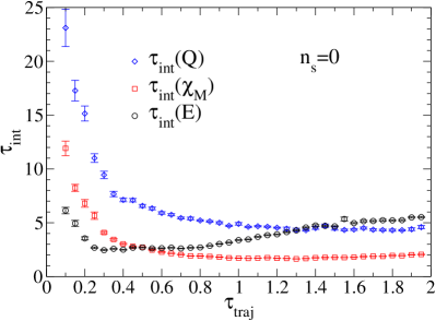
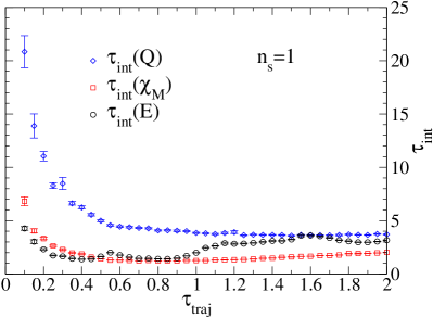
Figure 1: Integrated autocorrelation time $\tau_{\mathrm{int}}$ versus the trajectory length $\tau_{\mathrm{traj}}$ in CP⁹, $\beta=0.7$. $\tau_{\mathrm{int}}$ of the topological charge $Q$, the magnetic susceptibility $\chi_{M}$ and the energy $E$ is shown. Left side HMC without trivialization, right side THMC with one step of Euler integration $n_{s}$ and integration of the flow to $t_{T}=0.47$, such that the force is minimized. For both HMC and THMC a choice of the trajectory length around one is a good compromise.

4.1.1 Trajectory length

The effect of the trajectory length on the autocorrelation times for the CP⁹ model with $\beta=0.7$ can be found in Fig. 1. The left hand plot shows the HMC without trivialization, the right hand side the THMC with the leading order flow integrated up to $t_{T}=0.47$ (such that the force is minimized, as will be discussed later) with one Euler step ($n_{s}=1$). The step size $\epsilon=\tau/n_{\mathrm{step}}$ of the molecular dynamics trajectory integration is held approximately constant in all data points. (In all runs we targeted acceptance rates between 70% and 90%.) As already expected from the QCD experience, the optimal value of the trajectory length depends significantly on the observable. The energy $E$ decorrelates fastest, with a clear minimum at $\tau_{\mathrm{traj}}\approx 0.3$, whereas the magnetic susceptibility exhibits a very shallow minimum starting from $\tau_{\mathrm{traj}}\approx 1$. The topological charge $Q$ can profit from even longer trajectories. This is the case for the standard HMC as well as the one including the field transformation. Considering the computational costs of effectively decorrelated configurations, $\tau_{\mathrm{traj}}$ in the range between 0.5 and 1 seems to be efficient. We therefore choose $\tau_{\mathrm{traj}}=1$ for all $\beta$ in our main runs as a compromise. Although this might not be the optimal choice, it is a standard practice in QCD simulations.

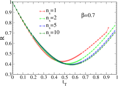
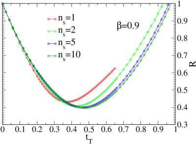
Figure 2: Reduction of the force in THMC compared to the force in HMC ($R=F_{THMC}/F_{HMC}$) depending on the integration length $t_{T}$ of the trivializing flow. Data are shown for CP⁹ with 1,2,5 and 10 steps of the Euler integration. Left side $\beta=0.7$, right side $\beta=0.9$. At large $t_{T}$, the curves are ordered as in the legend, $n_{s}=1$ at the top and $n_{s}=10$ at the bottom. The statistical errors are too small to be seen. The improvement for $n_{s}>1$ is negligible.

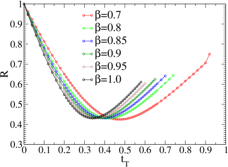
Figure 3: Force reduction $R$ versus the flow integration length $t_{T}$, only 1 step of Euler integration ($n_{s}=1$), for several values of $\beta$ in CP⁹. At small $t_{T}$, the curves are ordered as in the legend, $\beta=0.7$ at the top and $\beta=1.0$ at the bottom. As $\beta$ increases, the minimum moves towards smaller $t_{T}$, however, its depth does not change dramatically.

4.1.2 Integration of the flow

The second parameter to fix in our setup of the THMC is the value $t_{T}$ to which the flow Eq. (14) is integrated and the accuracy of the integration, which is given by the number of steps in the Euler integration. As a criterion, we use the reduction of the forces experienced in the molecular dynamics evolution, because perfect trivialization would result in forces equal to zero. The relative reduction of the force $R=F_{THMC}/F_{HMC}$ for $\beta=0.7$ and $\beta=0.9$ in the CP⁹ model is shown in Fig. 2. In both cases a reduction by about 60% can be reached at a value of $t_{T}$ around 0.5, much smaller than the $t_{T}=1$ for which trivialization is reached with the exact flow. The force reduction depends very little on the accuracy of the integration: whether 1, 2, 5 or 10 steps of the Euler integrator are used hardly matters. As shown in Fig. 3, the optimal value of $t_{T}$ decreases with increasing $\beta$, however, the reduction of the force at the minimum is almost constant, at least in the range $\beta=0.7,\dots,1.0$ which we have investigated.

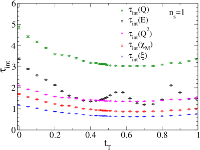
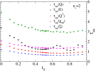
Figure 4: Integrated autocorrelation time $\tau_{\mathrm{int}}$ versus the integration length $t_{T}$ of the leading order trivializing flow, for CP⁹ with $\beta=0.7$. Left hand side: one step of Euler integration $n_{s}=1$. Right hand side: $n_{s}=2$. As shown in Fig. 2, maximum force reduction is obtained by $t_{T}=0.47$ ($n_{s}=1$) and $t_{T}=0.51$ ($n_{s}=2$), respectively.

Besides the reduction of forces, the field transformation is also supposed to reduce the autocorrelations experienced in the simulation. In Fig. 4 we therefore show the integrated autocorrelation time for different flow integration lengths $t_{T}$ for CP⁹ with $n_{s}=1$ and $n_{s}=2$. This can also be seen as a check of the force criterion depicted in Figs. 2 and 3. As expected, the optimum $t_{T}$ to minimize autocorrelations depends on the observable considered. Qualitatively, we observe that the force criterion leads to a good choice of $t_{T}$ with respect to reduction of the autocorrelation. However, while for larger values of $t_{T}$ the force ratio becomes worse, the autocorrelation shows a fairly flat behavior. This test was done at fixed molecular dynamics step size and therefore fixed cost per trajectory. The main reason for the autocorrelation time rising for large $t_{T}$ is the decreasing acceptance rate. Had we kept the acceptance rate constant (meaning increased costs for $t_{T}$ larger than the force minimum), the autocorrelation times would have decreased further, although not very much. We conclude that the force criterion is reasonable for tuning $t_{T}$ and we therefore used it throughout this study.

4.1.3 Total cost of the simulation

The reduction in the forces by about a factor two from the field transformation allows a larger molecular dynamics step size by about the same factor. In particular for larger values of $\beta$, this leads to the same acceptance rate for HMC and THMC, see Table 1 for details. In our implementation, an elementary leap-frog step of THMC with $n_{s}=1$ costs almost three times more than with HMC. More integration steps will further increase the cost. Together with the increased step size, this translates to roughly a factor of 1.5 increased cost per trajectory. In the next section, we will find a reduction of the autocorrelation times between roughly 1.5 and 1.8, depending on the observable. This means that the total cost of simulation for HMC and THMC with $n_{s}=1$ are about the same.

5 Results

With this setup, we performed extensive runs at correlation lengths between $\xi\approx 2.3$ and $\xi\approx 16.6$, using the plain HMC and compare it to the THMC with the flow integrated with $n_{s}=1$ Euler step. For the latter we use the optimal values of the flow parameter $t_{T}$ with respect to reduction of the force. The detailed parameters can be found in Table 1, expectation values of various observables in Table 2. The measured autocorrelation times in units of molecular dynamics time are listed in Table 3.

$\beta$	$L$	$n_{s}$	$\tau_{\mathrm{traj}}$	$n_{\mathrm{step}}$	$t_{T}$	$P_{\mathrm{acc}}$	stat. [MD time]
0.70	42	0	1	062	—	0.84	01000k
0.70	42	1	1	031	0.47	0.77	05000k
0.80	60	0	1	085	—	0.85	01000k
0.80	60	1	1	043	0.43	0.81	04346k
0.85	72	0	1	097	—	0.86	03682k
0.85	72	1	1	049	0.40	0.82	04230k
0.90	90	0	1	120	—	0.86	02418k
0.90	90	1	1	060	0.37	0.85	04114k
0.95	120	0	1	170	—	0.90	25282k
0.95	120	1	1	085	0.35	0.90	13110k
1.00	160	0	1	200	—	0.90	32763k
1.00	160	1	1	100	0.33	0.90	14408k

Table 1: Parameters of our runs in CP⁹ with coupling $\beta$ and lattices of size $L^{2}$. $n_{s}$ is the number of Euler integration steps, where zero corresponds to the standard HMC algorithm. $\tau_{\mathrm{traj}}$ denotes the integration length of the molecular dynamics trajectory, $n_{\mathrm{step}}$ its discretization, $t_{T}$ the integration length of the trivializing flow and $P_{\mathrm{acc}}$ the Metropolis acceptance rate. The last column gives the statistics in units of molecular dynamics time.

$\beta$	$L$	$n_{s}$	00$\xi$	000$E$	000$\chi_{M}$	$10^{5}Q^{2}/V$
0.70	42	0	2.312(3)	0.784378(16)	10.124(3)	470.6(1.4)
0.70	42	1	2.3117(12)	0.784361(6)	10.1278(12)	470.6(6)
0.80	60	0	4.602(6)	0.667028(10)	28.088(16)	97.6(8)
0.80	60	1	4.595(2)	0.667023(4)	28.068(6)	96.9(3)
0.85	72	0	6.389(5)	0.622276(4)	46.91(2)	46.0(4)
0.85	72	1	6.386(4)	0.622271(4)	46.916(14)	46.2(3)
0.90	90	0	8.816(11)	0.583835(4)	78.40(6)	23.3(5)
0.90	90	1	8.837(6)	0.583834(3)	78.49(3)	23.3(3)
0.95	120	0	12.134(7)	0.5502611(8)	131.39(5)	11.73(16)
0.95	120	1	12.132(7)	0.5502626(11)	131.41(5)	11.91(19)
1.00	160	0	16.607(12)	0.5205860(6)	220.48(12)	006.18(18)
1.00	160	1	16.601(14)	0.5205872(8)	220.37(13)	006.14(20)

Table 2: Expectation values of our runs in the CP⁹ model, $n_{s}$ is the number of Euler integration steps, further parameters are found in Table 1. We give results for the correlation length $\xi$, the energy, the magnetic susceptibility and the square of the topological charge.

$\beta$	$n_{s}$	$\xi$	$\tau(\xi)$	$\tau(E)$	$\tau(\chi_{M})$	$\tau(Q)$	$\tau(Q^{2})$
0.70	0	2.312(3)	1.181(8)	3.38(4)	1.71(2)	4.9(1)	2.10(2)
0.70	1	2.3117(12)	0.943(3)	1.981(8)	1.268(8)	3.86(2)	1.792(7)
0.80	0	4.602(6)	3.61(6)	3.60(6)	5.14(10)	35.3(1.2)	16.6(4)
0.80	1	4.595(2)	1.983(13)	2.99(4)	2.84(2)	27.0(4)	12.30(13)
0.85	0	6.389(5)	7.32(9)	3.83(6)	9.80(14)	126(4)	57.0(1.3)
0.85	1	6.386(4)	3.80(3)	3.62(5)	5.29(6)	95(5)	43.7(8)
0.90	0	8.816(11)	13.8(3)	3.86(9)	18.4(5)	527(38)	238(12)
0.90	1	8.837(6)	7.57(12)	3.73(4)	10.5(2)	345(17)	160(5)
0.95	0	12.134(7)	27.9(5)	3.86(11)${}_{-0.0}^{+0.3}$	40.5(8)	2260(120)	1080(40)
0.95	1	12.132(7)	16.3(4)	3.60(7)${}_{-0.0}^{+0.2}$	25.2(8)	1630(70)	800(30)
1.00	0	16.607(12)	67(3)	5.6(4)${}_{-0.0}^{+1.5}$	115(7)	13400(1100)	6300(400)
1.00	1	16.601(14)	38(3)	4.3(2)${}_{-0.0}^{+1.9}$	70(5)	9400(800)	3860(250)

Table 3: Auto-correlation times corresponding to Table 2. For $\beta=0.95$ and $\beta=1.0$, systematic errors for $\tau(E)$ account for the uncertainty in estimating the contribution of the tail of the auto-correlation function.

5.1 Critical behavior

This brings us to our main result, the critical slowing down of the simulations as $\beta\to\infty$. For large correlation length $\xi$, the autocorrelation times are expected to grow as

$$\tau_{\mathrm{int}}(A)\propto\xi^{z}$$ (20)

with $z$ the dynamical critical exponent. It depends, of course, on the observable $A$. This scaling is only expected for asymptotically large $\xi$, however, also with our limited range we can get an estimate of the severeness of the problem and the reduction brought by the field transformation. Since we have periodic boundary conditions, topological sectors are expected to form in the continuum limit. Because of the ensuing barriers in the free energy, Ref. [5] suggests for the topological charge an exponential behavior of the form

$$\tau_{\mathrm{int}}(Q^{2})\propto\exp(c\,\xi^{\theta})\ .$$ (21)

However, as we will see below, the presence of such an exponentially slow mode does also have an effect on all observables which do not completely decouple from it.

Figure 5: The integrated autocorrelation time of various observables for the HMC as a function of the correlation lengths. In this log-log plot, the dashed lines indicate the results of power law fits to the data for $4<\xi<13$. The solid line represents the the exponential form Eq. (21). The error bars are smaller than the size of the symbols.

In Fig. 5 we show the $\tau_{\mathrm{int}}$ of various observables as a function of the correlation length for the HMC algorithm without field transformation. As expected, the slowing down in the topological charge is much more severe than in the other observables which in the interval $4<\xi<13$ show a behavior compatible with the power law Eq. (20). Making statistically relevant statements about this is difficult, because the acceptance rates are not constant over all our runs. We try to compensate for that by considering $P_{\mathrm{acc}}\tau_{\mathrm{int}}$, but of course this is only a partial correction. Also the data is not expected to follow exactly the leading order scaling law; due to the high accuracy of our data next-to-leading orders might become visible. Nevertheless, fitting the data in the range of $4<\xi<9$ to Eq. (20), we get $z=2.0(1)$ for the magnetic susceptibility and for the correlation length. The errors are statistical only. The energy $E$ exhibits a very flat behavior in $2<\xi<13$ with $z=0.12(1)$. For $E$ and $\xi$, the fits have a $\chi^{2}$/dof between 1 and 3.3, which is acceptable considering the simple formula and the problems discussed above. However, while the behavior for $E$ and $\xi$ are compatible with a power law up to $\xi\approx 12.1$, the last data point at $\xi\approx 16.6$, and for $\chi_{m}$ also the point at $\xi\approx 12.1$, show a clear deviation. We interpret this as a consequence of a correlation between these observables and the topological charge and will discuss this issue below in detail.

The square of the topological charge exhibits a much worse scaling behavior than the other observables. Fitting Eq. (20) to the data with $4<\xi<12$ , we get $z\approx 4$, however, the agreement is not convincing and the $\chi^{2}$/dof$\;\approx 20$ is poor. The exponential function Eq. (21) works much better and delivers a good description of the data in the whole region $2<\xi<17$ with $c\approx 4.2$ and $\theta\approx 0.43$. It has $\chi^{2}$/dof$\;\approx 0.25$, but due to the problems discussed above, this has to be taken with care.

5.2 Effect of the slow modes

Having detected at least one very slow mode in the simulation raises the question to what extent the various observables are affected. The answer will depend both on the particular observable and the accuracy required in the simulation. We interpret the deviation from the power law scaling behavior of the energy, the magnetic susceptibility and the correlation length observed in Fig. 5 at $\xi\approx 16.6$ (and weakly already at $\xi\approx 12.1$) to be a consequence of the correlation between the slow mode and the observables. As observed in the topological charge squared, the time constant of this mode rises exponentially and at this point its contribution is no longer sufficiently suppressed by the smallness of the coupling to the observable and becomes noticeable.

If we identify, for a moment, the slow mode with the topological charge, one can understand the phenomenon with the following: while the simulation is trapped in one topological sector, it samples the observable restricted to that sector $A(Q)$. If the estimate obtained before moving on to another sector after about $\tau(Q)$ steps is more precise than variance $\Delta^{2}=\mathrm{var}_{Q}(A(Q))$ of $A(Q)$ over topological sectors, then the autocorrelation time will have a significant contribution from the topological modes. What matters thus is the relative size of $\sqrt{\mathrm{var}(A(Q))\tau_{\mathrm{int}}(A)/\tau_{\mathrm{int}}(Q^{2})}$ and $\Delta$. In our data we observe that while the former is larger than the latter for most of our data points, this ordering is reversed for the points at the largest correlation length. If one is interested in the level of accuracy given by $\Delta$, the simulation has to run over many $\tau_{\mathrm{int}}(Q^{2})$.

As discussed in Ref. [2], the slow modes also pose a problem for the accurate determination of the autocorrelation times themselves. By restricting the sum in Eq. (19) to some window $W$, a small in amplitude but potentially long tail is neglected. To illustrate this, we show the autocorrelation function of the magnetic susceptibility at $\beta=1$ for the HMC algorithm in Fig. 6. At the beginning, it falls quickly to $\rho(t)\approx 0.01$ but then develops a very long tail, a situation already described in Ref. [9]. The tail is compatible with a single exponential with a time constant equal to the exponential autocorrelation time extracted from $\rho_{Q^{2}}(t)$. This is indicated in the figure by the dashed lines. We can use this information for an improved estimate of the autocorrelation time[2]. The usual sum of $\rho(t)$ in only performed up to the point where the single exponential tail starts. The rest of the sum is substituted by the integral over the single exponential for which the largest observed time constant observed in all observables with the same parity is taken. In our situation this is $\tau_{\mathrm{exp}}(Q^{2})$. Since the HMC obeys detailed balance, this gives a strict upper bound for $\tau_{\mathrm{int}}$, provided that there are no modes which suffer from an even slower evolution.

Also for the correlation length and at $\beta=0.95$ a similar behavior can be observed. Even though the coefficients might seem small, the slow modes still have a sizable contribution because of the very large time constant. At $\beta=1$, this tail contributes roughly 30% to $\tau_{\mathrm{int}}(\xi)$ and 50% to $\tau_{\mathrm{int}}(\chi_{m})$; for $\beta=0.95$ the contribution of the tail is roughly 10% and 17%, respectively. The values of the autocorrelation time from estimating the contribution of the tail in this way lie within the $1\sigma$ error of the values given in Table 3 obtained by a summation to large values of $W$. In case of $\tau_{\mathrm{int}}(E)$, the improved estimator is significantly higher than the value obtained from the truncated sum. The single exponential dominates from $t\approx 150$, contributing roughly 10% (50%) at $\beta=0.95$ ($\beta=1$). We take the different values as upper and lower bounds and state the discrepancy as systematic error in Table 3. If the true value is close to the upper bound, the scaling of $\tau_{\mathrm{int}}(E)$ deviates from a power law already at $\xi\approx 12.1$. If we assume that the exponential growth in the time constant is not compensated by the decrease in the coefficient, this contribution will be even more pronounced when $\beta$ is increased further.

Figure 6: Normalized autocorrelation function for the magnetic susceptibility for the HMC algorithm at $\beta=1$. The dashed lines correspond to a single exponential whose time constant has been extracted from the autocorrelation function of $Q^{2}$. The coefficients have been adjusted such that the two lines contain the $1\sigma$ region around $t=1000$. This contribution accounts for roughly half the integrated autocorrelation time.

5.3 Performance of the field transformation

We finally come to the comparison between the HMC and THMC algorithm, and we show the reduction in autocorrelation time achieved through the introduction of the field transformation. In Fig. 7 we plot the ratio of the autocorrelation of our observables for the two algorithms. The correlation length and the magnetic susceptibility for which we observe a 40% reduction profit most from the field transformation. For the topology roughly a 25% reduction is found, the energy is almost unaffected, however, it shows a quite short $\tau_{\mathrm{int}}$ over the whole range of data. Note that for $\xi\approx 12.1$ and $\xi\approx 16.6$ the reduction of $\tau_{\mathrm{int}}(E)$ has to be taken with care due to its systematic uncertainty. All critical exponents of the THMC algorithm extracted from the range $4<\xi<13$ agree within uncertainties with the ones of HMC. Also the deviation from the scaling law at $\xi\approx 12.1$ and $\xi\approx 16.6$ is observed. The exponential behavior of $\tau_{\mathrm{int}}(Q^{2})$ is compatible with HMC within error bars as well. We can conclude that the field transformation does not affect the scaling of these variables in the investigated region.

Figure 7: Cost reduction in terms of autocorrelation time for the different observables brought by the field transformation.

As commented above, the improvement factor which we find is close to the additional cost of the simulation and therefore the two algorithms perform rather similarly. These findings do not seem to depend strongly on $N$, since we also did limited simulations in the CP²⁰, with essentially equal results.

6 Summary

Whether a modification to an algorithm actually improves its performance is often very difficult to predict. It therefore needs numerical simulations to study its effects. Here we investigated recently proposed field transformations which can lead to a speed-up in HMC simulations. Unfortunately, the result is negative. Although we observe a reduction in autocorrelation times, the scaling towards the continuum limit is not improved. The reduction in the forces, which can be used to increase the step size of the molecular dynamics integration, is compensated by the computational overhead of the method. However, this conclusion does not have to be universally true for all theories. In QCD with dynamical fermions, e.g., the computational cost of the construction would be a minor part of the whole cost of the simulation.

Investigating the pure HMC algorithm serves also as an illustration that exponentially slow modes will at some point affect other observables of the theory. The deviation at $\xi\approx 16$ from the scaling behavior, which we observe for the observables up to a correlation length of 12, is therefore a cautionary tale for QCD simulations. Even though the slow mode observed in the topological charge might not seem to have any influence on other observables in today’s simulations[2], at some point, the correlation to the topological charge can also affect the scaling behavior towards the continuum limit in these channels.

Acknowledgements

The calculations have been performed on local clusters at ZID at the University of Graz. We thank the institution for providing support. We are indebted to Christof Gattringer and Martin Lüscher for very valuable comments on a previous version of the paper and to Francesco Virotta for providing us with software for the analysis of autocorrelation functions. G.P.E. is grateful for the hospitality of the Computational Physics group of the Humboldt Universität zu Berlin and acknowledges support by the Doktoratskolleg DK W1203-N08 and the DFG project SFB/TR-55.

References

- [1] L. Del Debbio, H. Panagopoulos, and E. Vicari, dependence of SU() gauge theories, JHEP 0208 (2002) 044, [hep-th/0204125].
- [2] S. Schaefer, R. Sommer, and F. Virotta, Critical slowing down and error analysis in lattice QCD simulations, 1009.5228.
- [3] M. Lüscher, Trivializing maps, the Wilson flow and the HMC algorithm, Commun.Math.Phys. 293 (2010) 899–919, [arXiv:0907.5491].
- [4] S. Duane, A. D. Kennedy, B. J. Pendleton, and D. Roweth, Hybrid Monte Carlo, Phys. Lett. B195 (1987) 216.
- [5] L. Del Debbio, G. M. Manca, and E. Vicari, Critical slowing down of topological modes, Phys.Lett. B594 (2004) 315–323, [hep-lat/0403001].
- [6] M. Campostrini, P. Rossi, and E. Vicari, Monte Carlo simulation of CPN-1 models, Phys. Rev. D 46 (Mar, 1992) 2647–2662. 35 p.
- [7] E. Rabinovici and S. Samuel, The CPN-1 model: A strong coupling lattice approach, Physics Letters B 101 (1981), no. 5 323 – 326.
- [8] ALPHA Collaboration, U. Wolff, Monte Carlo errors with less errors, Comput. Phys. Commun. 156 (2004) 143–153, [hep-lat/0306017].
- [9] M. Lüscher, Topology, the Wilson flow and the HMC algorithm, PoS LATTICE2010 (2010) 015, [arXiv:1009.5877].