Azimuthal correlation of gluon jets created in proton-antiproton annihilation

Abstract

Annihilation process of proton and antiproton to guark antiquark pair accompanied by emission of two additional gluon jets with intermediate state of vector meson is considered. Strong azimuthal correlation is revealed of two gluonic jets, effectively created in the same plane. Some applications to cosmic ray events and to LHC experiments are discussed.

I Introduction

Now is widely believed that hard processes with hadron interaction at high energies can be described in frames of QCD. Contrary to photons in QED the QCD gluons can interact between themselves. The experimental check of nature of gluons become an important problem up to now. The dominant role of branching gluons was utilized in construction of the gluon dominance model (GDM) describing the events with large multiplicity in high energy collisions of leptons, (anti)protons and ions kok . Another indirect indication can be found in measuring the azimuthal correlations between gluon jets emitted by color quarks created in some hard hadronic process. It is the motivation of this paper to show that such kind of correlation take place in particular in process of annihilation of the high energy proton and antiproton to quark-anti quark with emission of two gluons.

Years ago in the paper of one of authors 1978 a problem of inelastic quark form factor was considered. The consideration was performed in the so called double-logarithmical approximation (DL) when the leading terms of order $(\alpha_{s}/\pi)^{2}(\ln(Q^{2}/m^{2}))^{4}$ was taken into account (here $Q^{2}=-q^{2}$ is the square of 4-momentum of virtual vector particle, $m$ is the effective mass of the gluon jet and $\alpha_{s}$ is QCD coupling constant). The one-loop radiative correction to the inelastic form-factor with a single hard gluon emission was found as well as the contribution from the channel of two hard gluons creation. It was confirmed, in particular, the S. Adler statement about cancelation of all DL enhancements when considering two-loop virtual corrections together with contribution of inelastic channels. Compared with QED case apart from some complication connected with the color properties of quarks and gluons, some additional kinematical regions arising from the existence of three gluon interaction vertex become to be important. It is the motivation of this paper to generalize the results obtained in 1978 year to the annihilation channel. Another reason is to search the possible relation with some azimuthal correlation of particles observed at LHC 2010 .

Some additional speculation can be done, a prediction about the character of energy distribution of cosmic rays of high energy cosmic . Really, taking into account the strong azimuthal correlation of jets created in high energy proton with nuclei in atmosphere (all the jets are in the same plane) a specific distribution of the spots of sets of the secondary particles of high energy can be measured: all these spots must be located along some lines-intersection line of production plane and the surface of the Earth.

Process of annihilation of proton and anti-proton to a vector meson with the subsequent creation of quark-anti-quark pair and two hard gluon jets

$$p(p_{+})+\bar{p}(p_{-})\to v(q)\to q(q_{-})+\bar{q}(q_{+})+g(k_{1})+g(k_{2})$$ (1)

in Born approximated is described by a set of Feynman diagrams of two kinds. One of them corresponds to emission of both gluons by quark and anti-quark and another contain the specific for QCD three gluon vertex, when two gluons arise from a single gluon, emitted by quark or anti-quark. We will use Sudakov parametrization for 4-momenta of the problem, introducing two light- like vectors

$$k_{i}=p_{1}\beta_{i}+p_{2}\alpha_{i}+k_{i\bot},k_{i\bot}p_{1,2}=0;k_{i\bot}^{2}=-\vec{k}_{i}^{2}<0;$$

$$p_{1}^{2}=p_{2}^{2}=0;s=(q_{+}+q_{-})^{2},p_{1}=q_{-}-\frac{1-\beta}{1+\beta}q_{+};p_{2}=q_{+}-\frac{1-\beta}{1+\beta}q_{-};$$

$$q_{+}^{2}=q_{-}^{2}=M^{2}=\frac{s}{4}(1-\beta^{2});$$

$$k_{i}^{2}=s\alpha_{i}\beta_{i}-\vec{k}^{2}=m^{2}.$$ (2)

Here $M$ is quark mass and $m$ is the mass of vector particle - gluon (or the invariant mass of the relevant gluon jet).

In terms of Sudakov variables the phase volume of two real soft gluons can be written in form

$$\frac{d^{3}k_{1}}{2\omega_{1}}\frac{d^{3}k_{2}}{2\omega_{2}}=d^{4}k_{1}\delta(k_{1}^{2}-m^{2})d^{4}k_{2}\delta(k_{2}^{2}-m^{2})=$$

$$\frac{s}{2}d\alpha_{1}d\beta_{1}d^{2}\vec{k}_{1}\delta(s\alpha_{1}\beta_{1}-\vec{k}^{2}-m^{2})\frac{s}{2}d\alpha_{2}d\beta_{2}d^{2}\vec{k}_{2}\delta(s\alpha_{2}\beta_{2}-\vec{k}^{2}-m^{2})=$$

$$(\frac{s}{2})^{2}\frac{d\phi_{1}}{2}d\alpha_{1}d\beta_{1}\theta(\alpha_{1}\beta_{1}-\gamma)\frac{d\phi_{2}}{2}d\alpha_{2}d\beta_{2}\theta(\alpha_{2}\beta_{2}-\gamma),$$ (3)

with $\gamma=m^{2}/s<<1$. For the ratio of matrix elements squared and summed on final state quantum numbers was obtained in 1978 :

$$\frac{\sum|M^{p\bar{p}\to q\bar{q}gg}|^{2}}{\sum|M^{p\bar{p}\to q\bar{q}}|^{2}}=(\frac{\alpha_{s}}{\pi})^{2}\times Z;$$

$$Z=\{(\frac{1}{\alpha_{2}\beta_{1}}+\frac{1}{\alpha_{1}\beta_{2}})\frac{1}{(\beta_{1}+\beta_{2})(\alpha_{1}+\alpha_{2})}(\frac{N^{2}-1}{2N})^{2}$$

$$+(-\frac{N^{2}-1}{4N^{2}})\{(\frac{1}{\alpha_{2}\beta_{1}}+\frac{1}{\alpha_{1}\beta_{2}})\frac{1}{(\beta_{1}+\beta_{2})(\alpha_{1}+\alpha_{2})}+\frac{1}{\alpha_{1}\alpha_{2}\beta_{1}\beta_{2}}\}$$

$$+\frac{(N^{2}-1)s}{4((k_{1}+k_{2})^{2}-m^{2})}\{\frac{1}{\alpha_{2}\beta_{1}}+\frac{1}{\alpha_{1}\beta_{2}}+\frac{1}{(\beta_{1}+\beta_{2})(\alpha_{1}+\alpha_{2})}\{-4+\frac{\alpha_{1}}{\alpha_{2}}+\frac{\alpha_{2}}{\alpha_{1}}+\frac{\beta_{1}}{\beta_{2}}+\frac{\beta_{2}}{\beta_{1}}\}\}\}$$

$$=A+\frac{s}{(k_{1}+k_{2})^{2}-m^{2}}B.$$ (4)

$N=3$ is the rank of color group $SU(N)$. Main contribution arises from two kinematical configurations in 4-dimensional manyfold $R$: $\gamma<\alpha_{i},\beta_{i}<1,\alpha_{i}\beta_{i}>\gamma$ with the additional conditions in the region $a$)

$$\alpha_{i}>>\alpha_{j},\quad\beta_{i}>>\beta_{j},\quad i,j=1,2$$

and region $b)$

$$1>>|\alpha_{1}\beta_{2}-\alpha_{2}\beta_{1}|>>\gamma.$$

Contribution of first kind kinematics, region $a)$, is

$$\frac{d\sigma^{p\bar{p}\to q\bar{q}gg}}{d\sigma_{0}}|_{a)}=\frac{1}{2!}(\frac{\alpha_{s}}{2\pi})^{2}\rho^{4}c_{F}^{2},\quad\rho=\ln(s/m^{2}),\quad c_{F}=\frac{N^{2}-1}{2N}$$ (5)

where $\alpha_{s}$ is gluon coupling constant and $d\sigma_{0}$ is the differential cross section of annihilation of proton and anti-proton to the pair of quark and anti-quark (see Appendix A).

But it is not a total answer. The double-logarithmic type contribution arises as well from the region $b)$. Really the denominator of the virtual gluon propagator

$$(k_{1}+k_{2})^{2}-m^{2}=2k_{1}k_{2}+m^{2}=s(\alpha_{1}\beta_{2}+\alpha_{2}\beta_{1})+m^{2}-2|\vec{k}_{1}||\vec{k}_{2}|\cos\phi=s(a-b\cos\phi),$$

$$\vec{k}_{i}^{2}=s\alpha_{i}\beta_{i}-m^{2}.$$ (6)

Being averaged on azimuthal angle $\phi$ it has a form

$$\int\limits_{-\pi}^{\pi}\frac{d\phi}{2\pi}\frac{1}{a-b\cos\phi}=\frac{1}{\sqrt{a^{2}-b^{2}}}.$$ (7)

Using the on mass shell conditions for gluons we have

$$\frac{1}{\sqrt{a^{2}-b^{2}}}=\frac{1}{\sqrt{(\alpha_{1}\beta_{2}-\alpha_{2}\beta_{1})^{2}+4\gamma[\alpha_{1}\beta_{2}+\alpha_{1}\beta_{1}+\alpha_{2}\beta_{2}]}}.$$ (8)

We see that in region $b)$ it is presented a quite different region of DL contributions to the cross section.

Performing the integration it was obtained ( 1978 expression (17)):

$$\frac{d\sigma^{(2)}}{d\sigma_{0}}=\frac{1}{2!}c_{F}(\frac{\alpha_{s}}{2\pi}\rho^{2})^{2}[c_{F}+\frac{1}{6}c_{V}].$$ (9)

Color structure containing $c_{V}=N$ violates Poisson distribution in emission of two colored vector particles

$$\frac{d\sigma^{(n)}}{d\sigma_{0}}=\frac{1}{n!}a^{n}e^{-a},\quad a=\frac{\alpha_{s}c_{F}\rho^{2}}{2\pi}.$$ (10)

Here factor with $exp(-a)$ takes into account the contributions from virtual vector meson emission.

We suggest to measure the azimuthal correlation in form

$$A(\phi)=\frac{d\sigma^{(2)(\phi)}}{\int\limits_{-\pi}^{\pi}d\sigma^{(2)}(\phi)d\phi}=$$

$$\frac{c_{F}^{2}+8c_{F}c_{V}\pi\frac{Z(\rho,\phi)}{\rho^{4}}}{2\pi(c_{F}^{2}+\frac{1}{6}c_{F}c_{V})}=\frac{4+72\pi\frac{Z(\rho,\phi)}{\rho^{4}}}{11\pi}.$$ (11)

Function $Z(\rho,\phi)$ satisfies the normalization condition $\int\limits_{-\pi}^{\pi}A(\phi)d\phi=1$

To obtain $Z(\rho,\phi)$ we simplify the expression $a-b\cos\phi$ in such a way:

$$\frac{1}{a-b\cos\phi}\approx\frac{2a}{a^{2}-b^{2}+a^{2}\phi^{2}},\quad a=2\alpha_{1}\beta_{2}.$$ (12)

Performing the $\alpha_{2}$ integration we obtain

$$\int\frac{d\alpha_{2}}{a-b\cos\phi}=\frac{4\pi\alpha_{1}\beta_{2}}{\beta_{1}^{2}}\frac{1}{\sqrt{R}}.$$ (13)

The quantity $R$ have a different form depending on integration regions. We obtain (see Figs. 2–4):

$$Z(\rho,\phi)=\int\limits_{m/\sqrt{s}}^{1}\frac{d\beta_{1}}{\beta_{1}}\int\limits_{m^{2}/(s\beta_{1})}^{\beta_{1}}\frac{d\alpha_{1}}{\alpha_{1}}\times\{\int\limits_{\sqrt{m^{2}\beta_{1}/(s\alpha_{1})}}^{\beta_{1}}\frac{d\beta_{2}}{\sqrt{R_{1}}}+\int\limits_{\beta_{1}}^{1}\frac{d\beta_{2}}{\sqrt{R_{2}}}\}+\int\limits_{m/\sqrt{s}}^{1}\frac{d\alpha_{1}}{\alpha_{1}}\int\limits_{m^{2}/(s\alpha_{1})}^{\alpha_{1}}\frac{d\beta_{1}}{\beta_{1}}\times\{\int\limits_{\sqrt{m^{2}\beta_{1}/(s\alpha_{1})}}^{\beta_{1}}\frac{d\beta_{2}}{\sqrt{R_{1}}}+$$

$$\int\limits_{\beta_{1}}^{\beta_{1}/\alpha_{1}}\frac{d\beta_{2}}{\sqrt{R_{2}}}\}.$$ (14)

with

$$R_{1}=\frac{4m^{2}}{s}\frac{\alpha_{1}}{\beta_{1}}+4(\frac{\alpha_{1}\beta_{2}\phi}{\beta_{1}})^{2};$$

$$R_{2}=\frac{4m^{2}}{s}\frac{\alpha_{1}\beta_{2}^{2}}{\beta_{1}^{3}}+4(\frac{\alpha_{1}\beta_{2}\phi}{\beta_{1}})^{2}.$$ (15)

We use the integrals

$$\int\limits_{\beta_{1}}^{1}\frac{d\beta_{2}}{\sqrt{R_{2}}}=\frac{\beta_{1}}{2\alpha_{1}}\frac{\ln(1/\beta_{1})}{\sqrt{\phi^{2}+\frac{m^{2}}{s\alpha_{1}\beta_{1}}}}$$

$$\int\limits_{\beta_{1}}^{\beta_{1}/\alpha_{1}}\frac{d\beta_{2}}{\sqrt{R_{2}}}=\frac{\beta_{1}}{2\alpha_{1}}\frac{\ln(1/\alpha_{1})}{\sqrt{\phi^{2}+\frac{m^{2}}{s\alpha_{1}\beta_{1}}}}$$ (16)

and

$$\int\limits_{\sqrt{\gamma\beta_{1}/\alpha_{1}}}^{\beta_{1}}\frac{d\beta_{2}}{\sqrt{R_{1}}}=\frac{\beta_{1}}{2\alpha_{1}|\phi|}\times$$

$$\{\ln(t|\phi|+\sqrt{1+t^{2}\phi^{2}})-\ln(|\phi|+\sqrt{1+\phi^{2}})\},t=\sqrt{\alpha_{1}\beta_{1}/\gamma}.$$ (17)

To express the result in terms of one-fold integrals we use

$$\int\limits_{\sqrt{\gamma}}^{1}\frac{d\beta_{1}}{\beta_{1}}\int\limits_{\gamma/\beta_{1}}^{\beta_{1}}\frac{d\alpha_{1}}{\alpha_{1}}F(t)=\frac{1}{2}\int\limits_{0}^{\rho}dy(\rho-y)F(\exp(y/2));$$

$$\int\limits_{\sqrt{\gamma}}^{1}\frac{d\beta_{1}}{\beta_{1}}\ln(1/\beta_{1})\int\limits_{\gamma/\beta_{1}}^{\beta_{1}}\frac{d\alpha_{1}}{\alpha_{1}}F(t)=\frac{1}{8}\int_{0}^{\rho}dy(\rho-y)^{2}F(\exp(y/2));$$

$$\int\limits_{\sqrt{\gamma}}^{1}\frac{d\beta_{1}}{\beta_{1}}\int\limits_{\gamma/\beta_{1}}^{\beta_{1}}\frac{d\alpha_{1}}{\alpha_{1}}=\frac{1}{2}\int_{0}^{\rho}dy(\rho-y)=\frac{1}{4}\rho^{2}.$$ (18)

The result is

$$Z(\rho,\phi)=\frac{1}{4}\int\limits_{0}^{\rho}(\rho-y)^{2}\frac{1}{\sqrt{\phi^{2}+e^{-y}}}dy+$$

$$\frac{1}{|\phi|}\int\limits_{0}^{\rho}(\rho-y)\ln(|\phi|e^{y/2}+\sqrt{1+\phi^{2}e^{y}})dy+O(\rho^{2}).$$ (19)

Function $Z(\rho,\phi)$ has a delta-function type behavior, concentrated in $|\phi|\sim\sqrt{s/m^{2}}$ with $Z(0)\approx 8\sqrt{s/m^{2}}$ and besides $\int\limits_{-\epsilon}^{\epsilon}Z(\phi)d\phi=(1/24)\rho^{4}$. Here $\sqrt{m^{2}/s}<<\epsilon<<1.$

This function is presented in Figure 1 for $\rho=10$.

II Discussion

Let remind the three dimensional picture in center of mass of initial particles. Hard quark and anti-quark of final state move back to back at large angles and emit two gluons. One of them moves close to quark direction another - close to anti-quark ones. Differential cross section on the azimuthal angle between the planes containing quark and the relevant gluon and the plane containing anti-quark and another gluon will have a isotropic part and one with sharp dependence distributed close to the value $|\phi|\approx O(\sqrt{\frac{m^{2}}{s}})$.

Energies of gluons are small compared with energies of quark-and anti-quark. This statement follows from the fact that the main,($\sim\rho^{4}$) contribution follows from the 4-vectors of gluons polarization in kinematics of isotropic contributions to the cross section are situated in the plane of quark and anti-quark 4-momenta $e_{i}=-\sqrt{\frac{\alpha_{i}}{s\beta_{i}}}p_{2}+\sqrt{\frac{\beta_{i}}{s\alpha_{i}}}p_{1}$, whereas the ones, responsible for azimuthal correlation are essentially situated in the plane transversal to quark momenta.

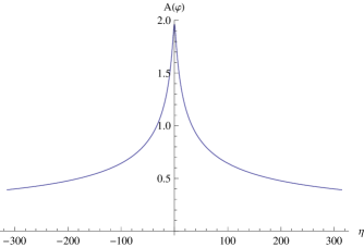
Fig. 1: the azimuthal distribution function $A(\phi)$ for $m^{2}/s=10^{-4}$, $\phi=\eta\sqrt{m^{2}/s}$ is presented.

For the case of production of additional soft quark-anti-quark instead of two gluon the DL enhancement factor do not appears.

The DL enhancement phenomena will take place for gluons emitted by any pair of colored fermions which have large invariant mass $\sqrt{s}>>m$. However the explicit form of $\phi$-independent and $\phi$-dependent parts of matrix element square (see (4)) will depend on mechanism of quark creation. In particular one can consider the peripheral mechanism of quark-anti-quark creation in collisions of hadrons by two reggeized gluons.

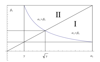
Fig. 2: Integration domain in $\alpha_{1}$, $\beta_{1}$ plane.

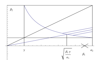
Fig. 3: Integration domain for I region (see Fig.2 )in $\alpha_{2}$, $\beta_{2}$ plane.

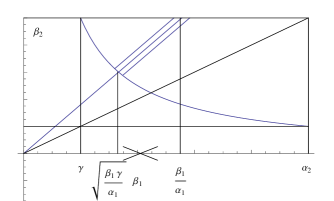
Fig. 4: Integration domain in $\alpha_{2}$, $\beta_{2}$ plane for II region (see Fig.2).

From the comparisons with experimental topological cross sections of $pp$ interactions and $p\bar{p}$ annihilation at the energy region close to U-70 accelerator (IHEP, Protvino) the estimations of the MGD-parameters were obtained kok . The mean number of hadrons formed from one gluon source at hadronization stage is added from the charged and neutral components (pions predominate): $\overline{n}_{tot}$=1.63+1.01=2.64. The invariant mass of such gluon sources may be determined as $m$= 2.64 $\times$ 0.139= 0.37 (GeV). At accelerator U-70 energy $\sqrt{s}$=11.6 GeV. The parameter $\rho$ will be equal to, $\rho=\ln\frac{s}{m^{2}}$=6.9. At that $\rho$ the noticeable peak may appear in the angular dependence too. It looks also as 1-GeV g-jet at low threshold of ISR-energy, $\sqrt{s}$=32 GeV. To describe the topological cross section widening at ISR energies the gluon fission was included at QCD-cascade stage in GDM kok . One can make next assumptions. To reveal the angular distribution peak appeared from gluon fission at the energy lower than LHC region it is enough to choose g-jets with smaller invariant mass m or determine mass of g-jet by means the peak. Also the estimation of the invariant gluon mass is compared to the mean transverse momentum of secondary particles at the relevant energies by the surprising way and this can be clue to ridge phenomenon understanding.

III Appendix A

Matrix element of process $p(p_{+})+\bar{p}(p_{-})\to v(q)\to q(q_{-})+\bar{q}(q_{+})$ have a form

$$M_{0}=\frac{g_{Vpp}g_{Vqq}F_{q}(q^{2})}{q^{2}-M_{V}^{2}}\bar{v}(p_{-})\Gamma_{\mu}u(p_{+})\times\bar{u}(q_{-})\gamma_{\mu}v(q_{+})$$ (20)

with phenomenal approach for the quark form factor and $g_{Vpp}=3g_{Vqq}\approx 9$, $V$ is dominantly $\omega$-meson.

Differential cross section have a form ($c=\cos\theta$, $\theta$ is the center of mass angle between the directions of motion of initial proton and the positively charged quark with momentum $q_{+}$)

$$\frac{d\sigma_{0}}{dc}=\frac{1}{2}\sigma_{0};$$

$$\sigma_{0}=\frac{N(G_{p}G_{q})^{2}}{2\pi s\beta(s-M_{V}^{2})^{2}}\beta_{q}R_{0},\beta_{q}=\sqrt{1-\frac{4m_{q}^{2}}{s}},$$

$$R_{0}=R_{1}|F_{m}|^{2}+\frac{2}{1-\tau}(|F_{m}|^{2}-|F_{e}|^{2})R_{2},$$ (21)

with $N=3$ is the number of quark colors

$$F_{m}=F_{1}+F_{2};F_{e}=F_{1}+\tau F_{2},\tau=\frac{s}{4M_{p}^{2}}$$ (22)

and

$$R_{1}=t^{2}+u^{2}+4s(M^{2}+m_{q}^{2})-2(M^{2}+m_{q}^{2})^{2};$$

$$R_{2}=tu+s(m_{q}^{2}-(M^{2}+m_{q}^{2})^{2}.$$ (23)

Here we use the kinematic invariants

$$s=(p_{+}+p_{-})^{2};t=(p_{+}-q_{+})^{2};u+(p_{+}-q_{-})^{2};s+t+u=2(M^{2}+m_{q}^{2}),$$ (24)

$M,m_{q}$-proton and quark masses. In paper F2 was argued that dominant contribution is provided by $V$-omega meson, and, besides $F_{2}^{\omega}=0$. In paper Fp the reasonable model for Dirac formfactor of proton in annihilation channel was suggested

$$F_{1}(s)=\frac{\Lambda^{4}}{\Lambda^{4}+(s-M_{p}^{2})^{2}}.$$ (25)

IV acknowledgements

One of authors (EAK) want to thank my collaborators Viktor Sergeevich Fadin and Lev Nikolaevich Lipatov for fruitful collaboration years ago. We are grateful to Azad Ahmadov for help. One of us (EAK) is grateful to Heisenberg-Landau 2011 fund for financial support. Besides EAK remind the 1978 year letter of LNL to him ”Greetings, Ed! About the problem of annihilation $e^{+}e^{-}$ to quarks and gluons. The important region of integration in process $e^{+}e^{-}\to q\bar{q}+ng$ depends on the kinematics of gluons emitted. Every new gluon moves in the direction of quark (anti-quark) or in the direction of parent quark, having the energy much less the one of it’s parent. Every gluon have it’s genealogical tree…”. In this way the correlations in the polar angle can be investigated. The authors express deep recognition to V. A. Nikitin for stimulating discussions of these studies.

References

(1)
V. I. Kuvshinov and E. S. Kokoulina, Acta Phys. Polon. B 13,
533 (1982); E. S. Kokoulina and V. A. Nikitin. in The
International School-Seminar The Actual Problems of Microworld
Physics, Gomel, Belarus, Dubna, 1, 221 (2004); E. Kokoulina,
Acta Phys.Polon. B 35, 295 (2004); E. S. Kokoulina and
V. A. Nikitin,
in Proceedings of Baldin Seminar on HEP Problems
“Relativistic Nuclear Physics and Quantum Chromodynamics”, JINR,
Dubna, Russia. p. 319, p. 327 (2005).
(2)
E. A. Kuraev and V. S. Fadin,
Yad. Fiz. v 27, (1978), p 1107.
(3)
The CMS Collaboration, Hep-ex 21 Sept 2010, arXiv:1009.4122v1.
(4)
R. A. Mukhamedshin, Phys.Part.and Nucl.Letters, 3, (2006)
p. 234.
(5)
R. Machleidt, PRC 63,024001 (2001).
(6)
C. Fernandes-Ramires et al, Ann. Phys. 321,1408 (2006).