Total and inelastic cross-sections at LHC at $\sqrt{s}=7\ TeV$ and beyond

Abstract

We discuss expectations for the total and inelastic cross-sections at LHC CM energies $\sqrt{s}\ =\ 7\ TeV$ and $14\ TeV$ obtained in an eikonal minijet model augmented by soft gluon $k_{t}$-resummation, which we describe in some detail. We present a band of predictions which encompass recent LHC data and suggest that the inelastic cross-section described by two channel eikonal models include only uncorrelated processes. We show that this interpretation of the model is supported by the LHC data .

I Introduction

Models for the high energy behaviour of the total cross-section hold a large interest since Heisenberg’s early attempts to describe the production of mesons through a shock wave mechanism Heisenberg (1952). The recent measurement of the inelastic cross-section at c.m. energy of 7 TeV by the ATLAS Aad et al. (2011) collaboration, together with preliminary CMS results cms (2011) and the expected results from other LHC groups, have renewed the interest in the subject Achilli et al. (2011); Block and Halzen (2011); Goulianos (2011); Jenkovszky et al. (2011). In addition, very recently, the TOTEM collaboration has released values for the total, the elastic and the inelastic cross-sections Latino et al. (2011) and the Auger experiment has given a measurement of the $p-air$ cross-section at $\sqrt{s}=57\ TeV$ Abreu et al. (2011).

The interest arises because total cross-sections access the large distance regime of particle interactions, i.e. a region where a QCD description is still lacking. In this paper, we present estimates for the total and the inelastic cross-sections at the LHC energies, $\sqrt{s}\ =\ 7\$ and $14\ TeV$, based on an eikonal minijet model augmented by soft-gluon resummation which we have developed over the years Corsetti et al. (1996); Grau et al. (1999); Godbole et al. (2005). Our present aim is not to give newer fits to the data, but to use the model to further develop an understanding of the underlying large distance dynamics. This has led us to an interesting result, discussed in this paper, namely that the expression for the inelastic cross-section obtained from simple two channel eikonal models only describes the contribution of uncorrelated scattering processes.

The eikonal model for high energy scattering Glauber (1959); Glauber and Matthiae (1970) provides a framework which incorporates unitarity in the description of scattering processes and can be used to describe both the total and the inelastic cross-section. Following up on the earliest discussions of the role of low $p_{t}$ jets (aka mini-jets) in affecting the energy dependence of total cross-sections Cline et al. (1973); Gaisser and Halzen (1985); Pancheri and Srivastava (1986), we have used the eikonal model to study the role of mini-jets in a QCD based framework, using as much as possible standard QCD phenomenological inputs, and techniques. Our model gives a description of the data on total cross-sections in terms of various QCD inputs at Leading Order (LO). It is able to address two major characteristics of the total cross-section, namely the sudden, power-like rise with energy at the ISR and the subsequent levelling off as needed by the Froissart bound.

Our LO description of the rise is based on LO parton density functions and LO parton-parton cross-sections, implemented by soft gluon resummation of the initial state radiation, which in turn is parametrized through the same LO PDF used for the mini-jet calculation. Non-leading effects in the resummation are incorporated in a non-perturbative ansatz for the singular, but integrable, coupling of soft gluons in the infrared region. Our model uses these inputs to obtain results for the total and the inelastic cross-section which are compared to the Tevatron and LHC energies. We notice that the inelastic cross-section poses yet another challenge, as the theoretical framework in which to model this quantity is not as easily defined as is the case for the total cross-section. We discuss this point in connection with eikonal models.

The plan of this paper is as follows. In Sec. II we discuss some features of the basic eikonal mini-jet model, and discuss the limitations of the two channel eikonal model. In Sec.  III we briefly summarise the relevant details of our model, which includes soft gluon $k_{t}$-resummation, and in Sect. IV we present numerical results on the total cross-section and some of the quantities which crucially control its energy dependence. In Sect. V we apply our model to calculate the inelastic cross-section and discuss the range of model parameters required to obtain an adequate description of currently available data for both the total and inelastic cross-sections at $7$ TeV and beyond. Our results are then compared with existing data and recently measured total and inelastic cross-sections at LHC. We end in Sect. VI with a comment on the limitations of eikonal models in describing total and inelastic cross-sections.

II Total and inelastic cross-sections in Eikonal mini-jet models

Eikonal mini-jet models are an extension of Glauber’s theory of diffractive scattering Glauber and Matthiae (1970), with the high energy dependence driven by QCD processess, such as production of low-$p_{t}$(mini) jets. In addition to proton-proton scattering Durand and Hong (1987); Durand and Pi (1989) and $p-air$ processes Durand and Pi (1988); Margolis et al. (1988), the eikonal minijet models have been applied to photon processes Fletcher et al. (1992); Honjo et al. (1993). QCD inspired versions Block et al. (1999, 2000) have been used to provide a unified description of proton and photon processes. Our version of the eikonal mini-jet model uses LO parton densities, determined from Deep Inelastic Scattering (DIS) and QCD evolution, and includes soft gluon $k_{t}$-resummation as a crucial component to access the very large distances probed by total cross-sections. Our model has been used to analyse total cross-sections for $pp$ and $p\bar{p}$ Godbole et al. (2006); Achilli et al. (2008), $\pi N$ and $\pi\pi$ Grau et al. (2010), $\gamma N$ Godbole et al. (2009) and $\gamma\gamma$ Godbole and Pancheri (2001); Godbole et al. (2008), and is shown to give a satisfactory description of the high energy behaviour of available data.

Eikonal models are formulated in the b-space representation of the scattering amplitude

$$F(s,t)=\int d^{2}{\bf b}f(b,s)=i\int d^{2}{\bf b}e^{i{\bf q}\cdot{\bf b}}[1-e^{i\chi(b,s)}]$$ (1)

One then gets in impact parameter space

$$\frac{d^{2}\sigma_{elastic}}{d^{2}{\bf b}}=|1-e^{i\chi(b,s)}|^{2}$$ (2)

Use of the optical theorem gives

$$\sigma_{total}=2\int d^{2}{\bf b}{\Re e[1-e^{i\chi(b,s)}]}=2\int d^{2}{\bf b}[1-\cos\Re e\chi(b,s)e^{-\Im m\chi(b,s)}]$$ (3)

With the above equations, and defining $\sigma_{inel}=\sigma_{total}-\sigma_{elastic}$ one obtains the total inelastic cross-section as

$$\sigma_{inel}=\int d^{2}{\bf b}[1-e^{-2\Im m\chi(b,s)}]$$ (4)

The above equation presents the possibility of calculating the imaginary part of the eikonal function $\chi(b,s)$, by relating it to the average number of independent inelastic collisions at given values of impact parameter b and c.m. energy $\sqrt{s}$. It is in fact possible to obtain the above expression for the inelastic total cross-section through a semi-classical argument, based on the hypothesis that the scattering between hadrons takes place through multiple parton-parton collisions which are independently distributed. This corresponds to assuming a Poisson distribution around an average number of collisions ${\bar{n}}$, namely

$$P(\{n,{\bar{n}}\})=\frac{({\bar{n}})^{n}e^{-{\bar{n}}}}{n!}$$ (5)

One then calculates the scattering at each impact parameter value $b$ between the scattering hadrons and integrates over the impact parameter space. Explicitly,

$$\sigma_{inel}(s)=\sum_{n=1}\int d^{2}{\bf b}\ P(\{n,{\bar{n}}\})=\int d^{2}{\bf b}[1-e^{-{\bar{n}}(b,s)}]$$ (6)

Comparing Eq.( 4) with Eq.(6) allows the identification ${\bar{n}}(b,s)=2\Im m\chi(b,s)$. Building a model for the average number of inelastic collisions then leads to $\Im m\chi$ and to making a model for the total cross-section as well. In particular, by putting $\Re e\chi(b,s)\approx 0$ in Eq. (3), one gets

$$\sigma_{tot}(s)=2\int d^{2}{\bf b}[1-e^{-{\bar{n}}(b,s)/2}]$$ (7)

and

$$\sigma_{el}(s)=\int d^{2}{\bf b}[1-e^{-{\bar{n}}(b,s)/2}]^{2}.$$ (8)

Such simple mini-jet models, as described above, can be used successfully to describe the total cross-section but the parameters, which allow to reproduce correctly the energy dependence of the total cross-section, predict inelastic cross-sections which are generally too small. Correspondingly, they predict elastic cross-sections too large and one needs further input to reproduce the differential elastic cross-section. An explanation, put forward in Lipari and Lusignoli (2009), is that a simple description of the scattering in terms of just two channels, elastic and inelastic, or elastic and total, is not adequate and that (single and double) diffractive channels need to be treated separately. To avoid introducing more parameters, one can insist on a two-channel model, as in Eqs. (6), (7) and (8), but in such case the inelastic cross-section, calculated through these equations in the eikonal mini-jet model, would not include correlated processes. The reason for this comes from comparing Eqs.  (4) and (6), which show that the inelastic formula, Eq. (4), includes only those processes where the underlying dynamics contains no correlations between collisions.

The above observation deserves a brief consideration. Many models, which use the eikonal framework, apply Eqs.  (4) and (3) to calculate the inelastic cross-section. The above discussion shows that, in so doing, the result will miss the contribution of correlated processes, such as diffraction. This is particularly important when extracting total cross-section data from cosmic ray experiments, which measure the inelastic $pp$ cross-section Anchordoqui et al. (2004). Another case, where the inelastic cross-section matters, is the calculation of the Survival Probability for Large Rapidity Gaps Bjorken (1993). Such models, Block and Halzen (2001, 2011) or our own Godbole et al. (2006), use the probability for occurence of no inelastic collisions in $b$-space, and caution must be exerted in interpreting what type of processes are excluded.

We shall return to this point at the end of the paper and investigate it in detail in future work. In the meanwhile, we present the results we obtain with the model described by Eqs. (6), (7) and (8) and study the role played by the parameters in describing total and inelastic cross-sections. We shall then compare our results with the recent ATLAS Collaboration Aad et al. (2011) analysis of inelastic collisions at LHC c.m. energy $\sqrt{s}=7\ TeV$, as well as with the preliminary CMS results cms (2011) and with the TOTEM value for the total cross-sectionLatino et al. (2011).

III The eikonal minijet model with soft $k_{t}$-resummation

The average number ${\bar{n}}(b,s)$ of collisions can be written as the number of scattering centers per unit area $A(b,s)$ multiplied by the scattering cross-section $\sigma(s)$, schematically $A(b,s)\sigma(s)$. In the parton model, we need both (i) the various parton-parton cross-sections as well as (ii) the parton densities for an evaluation of $A(b,s)$, $\sigma(s)$ and hence ${\bar{n}}(b,s)$.

In minijet models, the rise of the total cross section with energy is related to the increasing probability of perturbative low-x parton-parton collisions. Defining as $p_{tmin}$ the threshold for perturbative treatment of parton-parton scattering, this partonic contribution to $\sigma(s)$ can be calculated as

$$\sigma^{AB}_{\rm jet}(s;p_{tmin})=\int_{p_{tmin}}^{\sqrt{s}/2}dp_{t}\int_{4p_{t}^{2}/s}^{1}dx_{1}\int_{4p_{t}^{2}/(x_{1}s)}^{1}dx_{2}\sum_{i,j,k,l}f_{i|A}(x_{1},p_{t}^{2})f_{j|B}(x_{2},p_{t}^{2})~{}~{}\frac{d\hat{\sigma}_{ij}^{kl}(\hat{s})}{dp_{t}}.$$ (9)

Here, $i,\ j,\ k,\ l$ denote the partons and $x_{1},x_{2}$ the fractions of the parent particle momentum carried by the parton. $\sqrt{\hat{s}}=\sqrt{x_{1}x_{2}s}$ and $\hat{\sigma}$ are the center of mass energy of the two parton system and the hard parton scattering cross–section respectively. The numerical evaluation of this quantity strongly depends upon $p_{tmin}$ and the chosen set of Parton Density Functions (PDFs).

The minijet model is moot regarding the region $p_{t}<p_{tmin}$, and the underlying formalism is well defined only for perturbative values of momenta of the scattered partons for $p_{t}>p_{tmin}$. To take into account processes for which $p_{t}^{outgoing\ parton}<p_{tmin}$, one can split ${\bar{n}}$ into a soft and a hard part. i.e.

$${\bar{n}}(b,s)={\bar{n}}_{soft}(b,s)+{\bar{n}}_{hard}(b,s)$$ (10)

We then factorize each term into an overlap function $A(b,s)$ and a cross-section $\sigma(s)$, as

$${\bar{n}}_{soft/hard}(b,s)=A_{soft/hard}(b,s)\sigma_{soft/hard}(s)$$ (11)

The subscript hard is meant to indicate the perturbative origin of the mini-jet contribution to $\sigma_{total}(s)$ in calculating ${\bar{n}}(b,s)$, as given by Eq. (9). To proceed further in the calculation of ${\bar{n}}(b,s)$, one needs to supplement this simple model with the knowledge of density of partons in impact parameter space as well as a model for ${\bar{n}}_{soft}(b,s)$. These issues will be discussed below and in the next section.

III.1 Overlap functions in the transverse space

In the earliest discussions of eikonal models Durand and Pi (1989), $A(b,s)$ was taken to be independent of $s$ and was obtained by taking the convolution of the Fourier transform of the form factors (FF) of the colliding particles $A,B$, given by

$$A^{AB}_{FF}(b)=\int{{d^{2}{\bf q}}\over{(2\pi)^{2}}}{\cal F}^{A}(q){\cal F}^{B}(q)e^{i{\bf q}\cdot{\bf b}}$$ (12)

However, these simple parametrisations of the overlap function $A(b,s)$, augmented with a model for $n_{\rm soft}(b,s)$ failed to reproduce correctly the observed energy dependence Grau et al. (1999). When using in $\sigma_{jet}$ standard parton densities determined from Deep Inelastic Scattering (DIS), one found an energy rise that was either too fast or started too early. An acceptable description of the data, from the beginning of the rise to the TeVatron energies, was not possible without modifying the parton densities in an ad hoc manner.

We were able to obtain a good description of the energy behaviour using soft-gluon $k_{t}$-resummation, in a model (BN) labelled after Bloch and Nordsieck Bloch and Nordsieck (1937). It reflects the idea that any description of the scattering process between charged particles needs to include an infinite number of soft quanta in order to obtain a finite result. This model provides an energy dependent form factor, with the energy dependence introduced through the kinematics of single soft gluon emission in the $2\rightarrow 2$ parton-parton collision. In the BN model, the parton distribution in $b$-space, is determined as the Fourier transform of the probability, $d^{2}P(\bf K_{t})$, that the initially collinear parton-parton pair acquire, in the collision, an overall imbalance of transverse momentum ${\bf K}_{t}$ from emission of an indefinite number of soft gluons. We proposed

$$A_{BN}(b)=N\int d^{2}P({\bf K}_{t})e^{i{\bf K}_{t}\cdot{\vec{b}}}$$ (13)

with the condition $\int d^{2}{\bf b}A_{BN}(b)=1$.

The soft gluon transverse momentum distribution can be written as

$$d^{2}P({\bf K}_{t})=d^{2}{\bf K}_{t}\int\frac{d^{2}{\bf b}}{(2\pi)^{2}}exp[-i{\bf K}_{t}\cdot{\bf b}-h(b,q_{max})]$$ (14)

where $q_{max}$ is the appropriate scale for single soft gluon emission and the regularized function $h(b,q_{max})$ describes the overall soft gluon spectrum integrated over all possible values, up to $q_{max}$, i.e.

$$h(b,q_{max})=\int d^{3}{\bar{n}}_{g}(k)[1-e^{i{\bf k}_{t}\cdot\bf b}]\propto\int^{q_{max}}d^{2}{\bf k}_{t}\frac{\alpha_{s}(k_{t})}{k_{t}^{2}}[1-e^{i{\bf k}_{t}\cdot{\bf b}}]\ln\frac{2q_{max}}{k_{t}}$$ (15)

Eq. (14) was proposed in Pancheri-Srivastava and Srivastava (1977) for soft emission. In its application to hard QCD processes, such as lepton pair production in Dokshitzer et al. (1978); Parisi and Petronzio (1979), an expression for $h(b,q_{max})$ was proposed in which the integral of Eq. (15) extends only down to a QCD scale $\mu$. This allowed the use of the usual Asymptotic Freedom expression (AF) for $\alpha_{s}$ ($\alpha_{s}^{AF}$), safely neglecting the second term in the square bracket in Eq. (15). The proposal in Dokshitzer et al. (1978) has been used extensively in phenomenological analyses and can be traced back also to Sudakov (1956), and the resulting expression for $d^{2}P({\bf K}_{t})$ is usually referred to as the Sudakov form factor. For processes dominated by large distances, we have proposed that the $k_{t}$ integration be extended down to zero Nakamura et al. (1984). Of course this calls for the use of an appropriate form for the coupling of soft gluons to the emitting quarks, when $k_{t}\rightarrow 0$ in Eq.  (15). This strong coupling in the infrared region must be such as to give rise to an integrable spectrum. We have discussed this in our papers, in particular in Corsetti et al. (1996); Godbole et al. (2005) and more recently in Grau et al. (2009).

From Eqs. (13) and (14), our expression for $A(b,s)$, the normalized Fourier transform of the soft gluon resummed transverse momentum distribution, is

$$A_{BN}(b,s)=\frac{e^{-h(b,q_{max})}}{\int d^{2}{\bf b}e^{-h(b,q_{max})}}$$ (16)

where the dependence of $A_{BN}(b,s)$ on the center of mass energy arises through the kinematic quantity $q_{max}$. In our simplified version of the model proposed in Corsetti et al. (1996), this is obtained by averaging over the parton densities. Thus, the rising -high energy part- of the average number of collisions, is written as

$${\bar{n}}_{hard}(b,s)=A_{BN}(b,s)\sigma_{jet}(s,p_{tmin})$$ (17)

III.2 Scales and parameters

While we refrain from giving many details of the model, as they have been discussed carefully in our different publications Grau et al. (1999); Godbole et al. (2005); Grau et al. (2010), it is necessary that we give a brief discussion of the crucial parameters and the different scales involved, so that the physics issues become clear. Along with $p_{t}$, the transverse momentum of the partons involved in the basic $2\rightarrow 2$ scattering, another transverse momentum variable of relevance is $k_{t}$, the transverse momentum of the soft gluons emitted during the hard scattering process. This somewhat artificial separation, allows a clear delineation of different theoretical issues involved. The role of $p_{tmin}$ in the calculation of the hard part of the partonic cross-sections has been already explained. For the variable $k_{t}$, an important role is played by $q_{max}$, the maximum value allowed to single soft gluon emission during the collision between two partons. Using the kinematics of single gluon emission, this quantity can be written as

$$q_{max}({\hat{s}},y,Q^{2})=\frac{\sqrt{{\hat{s}}}}{2}(1-\frac{Q^{2}}{{\hat{s}}})\frac{1}{\sqrt{1+z\sinh^{2}y}}.$$ (18)

Here, $Q^{2}$ is the squared invariant mass of the outgoing parton pair, each parton with transverse momentum $p_{t}$. In the no-recoil approximation, $z=Q^{2}/{\hat{s}}$ and $y$ is the rapidity of the outgoing partons Chiappetta and Greco (1981). This scale, which affects the final result mostly through logarithms, is a semi-hard scale akin to $p_{tmin}$ and it is also of the same order of magnitude.

Depending on the energy scale of the process, as discussed at length in Grau et al. (1999), the calculation of the emission of soft gluons of momentum $k_{t}\leq q_{max}$ requires a special treatment. In our model, in order to be able to describe very large distance contributions to the total cross-sections, we have retained the second term in the square bracket in Eq. (15). Thus, yet another scale, in the problem at hand, is the impact parameter $b$ and special care is needed in discussing the effects in the infrared region when $k_{t}b\sim 1$. When $b$ becomes very large and $k_{t}\leq 1/b<\Lambda_{QCD}$, the calculation of $h(b,q_{max})$, and hence the overlap function, requires an ansatz for the behaviour of $\alpha_{s}$ in the far infrared where one can not use the usual expression at large scales. In the infrared region, our ansatz is to use

$$\alpha_{eff}=\alpha_{s}^{IR}=c\left({\Lambda^{2}_{QCD}}\over{k_{t}^{2}}\right)^{p}$$ (19)

namely an expression which is singular but integrable, provided $p<1$. We stress here that to access very large distances, we consider the very soft gluons for which $k_{t}\rightarrow 0$, which in turns implies resummation and, in the continuum limit, integration. Thus what matters is not the limit of the coupling for one soft gluon, but the integrability, a concept also put out by Dokshitzer Dokshitzer (1998) and used in jet analysis Dokshitzer et al. (1999).

As discussed below, the expression in Eq. (19) mimics the confinement dynamics. To perform the full integral of Eq. (15), which spans from the infrared to the beginning of the AF region, we then use an interpolating expression for $\alpha_{s}$, which reduces to the correct AF limit at large scales and to Eq. (19) in the infrared region Corsetti et al. (1996).

The parameter $p$ captures the physics at scales $k_{t}\lesssim\Lambda_{QCD}$ and affects the high energy behaviour of the total cross-section in a complex manner. As shown in  Grau et al. (2009), its value has to be between $1/2$ and $1$. As a consequence, the very large b-limit of the function $A_{BN}(b,s)$, i.e.

$$A_{BN}(b,s)\sim e^{-h(b,s)}\sim e^{-(\bar{\Lambda}b)^{2p}}$$ (20)

shows the impact parameter distribution falling at its fastest as a gaussian ($p=1$) and at its slowest as an exponential ($p=1/2$). The scale $\bar{\Lambda}\propto\Lambda_{QCD}$ includes a mild energy dependence through the scale $q_{max}$, as well as a residual dependence upon the parameter $p$. This behavior in impact parameter space joined with the high energy behaviour of the mini-jet cross-sections, $\sim s^{\varepsilon}$, was shown to lead to an asymptotic behaviour of the total cross-section consistent with the Froissart bound, namely

$$\sigma_{T}\approx\frac{2\pi}{{\bar{\Lambda}}^{2}}[\varepsilon\ln\frac{s}{s_{0}}]^{1/p}$$ (21)

upto leading terms in ($\ln s$) Grau et al. (2009).

III.2.1 About the singularity parameter $p$

Let us briefly discuss the physics implications of the choice of a particular value of the singularity parameter $p$. In our model, $p$ describes how singular $\alpha_{eff}$ is in the IR region and can be related to confinement dynamics. This is seen through the spatial-potential obtained through the Fourier transform of the one-gluon exchange potential generated by our effective coupling, namely

$$V(r)\sim r^{2p-1}\ \ \ \ \ \ r\rightarrow\infty$$ (22)

For $p=1/2$ the dressed one-gluon exchange potential is (essentially) a constant , whereas for $p=1$ it is linearly rising. In  Grau et al. (2009), we showed that the parameter $p$ has to be between $1/2$ and $1$, so that the corresponding potential is confining and $\alpha_{eff}$ at small scales is singular but integrable. On the other hand, given our ignorance of the actual confinement dynamics, we shall use it as a free parameter which can interpolate between a fully confining potential, linearly rising when $p=1$, and the inelastic scenario, in which partons are free to hadronize, with $p=0.5$ and the potential constant at infinity.

What we have given above is certainly too simple an argument, but it is not in contradiction with our understanding of the role played by the infrared singularity. From our phenomenology of the total cross-section Godbole et al. (2006); Achilli et al. (2008); Grau et al. (2010); Godbole et al. (2009), we have found that the value $p\sim 3/4$ gives acceptable descriptions of high energy data. Such a value would then be consistent with a rising potential.

III.2.2 About the PDFs

We consider the PDFs in our model to be phenomenological QCD parameters through which we describe the two high energy effects which are input to the eikonal: the rise at the beginning and the slowing down towards asymptotia. So far, ours is a Leading Order (LO) description of these two effects. In our parametrization of these effects we use LO densities able to go down to very small x-values and $Q^{2}\sim 1\ GeV^{2}$ (see below). In our first application of the model in Grau et al. (1999), we have found that GRV densities Gluck et al. (1992), when combined with our resummation expressions, provide a parametrization of the mini-jet effects which leads to a good description of total cross-section data. Through the years, other LO PDFs and many NLO and NNLO pametrizations have appeared. To use some of them in our model would be inconsistent and imply major modifications, as we explain below. Yet another possibility will be to employ the LO* distributions Sherstnev and Thorne (2008), suggested for use with the LO Monte Carlos. In future work, this and other possibiilties will be examined. Here we present the reasonably good LO description of the total cross-section, obtained so far in our model in terms of the various inputs such as LO PDFs, $p_{tmin}$ and $p$, and show how far it can take us in probing the long distance behaviour of QCD.

To be of significance in QCD descriptions of scattering processes, mini-jet models should use Parton Density Functions determined from Deep Inelastic Scattering. There are many PDFs, and not all of the available sets can be used in a model like ours, in which the rise of the total cross-section is due only to mini-jets. To have the rise appearing already at ISR energies, one needs $Q_{0}^{2}=p_{tmin}^{2}\simeq 1\ GeV^{2}$ and the PDFs we use must be valid down to such a low $Q_{0}^{2}$ value. Notice that we can only use LO PDFs, because in our model, the bulk of NLO contribution comes from soft gluon resummation, and using NLO versions might produce a double counting. The chosen PDFs must also be able to describe very low values of $x$, the energy fraction carried by the incoming partons. In particular most important are the low-$x$ gluon densities. Notice however that as the energy increases and lower and lower $x$-values are accessed, soft gluon resummation softens and tames the rise of low-$x$ gluon contribution. This contribution is not included in the low-$x$ phenomenology of current PDFs and this may pose a problem since the low $x$-behaviour of existing densities is modified by our model resummation inputs. The claim for instance that the low $x$-behaviour of some of the densities such as GRV is wrong, needs to be seen in light of resummed contributions like the ones we are considering : soft gluon effects are a NLO effect, but resummation to all orders down into the infrared is not included in the low-x behaviour of PDFs, neither in the LO nor in the NNLO parametrizations. Since such effects, in our opinion, are crucial for inclusion of QCD in descriptions of the total cross-section, we have resorted to use only LO parametrizations for all QCD effects. Even resummation is treated to LO order, since the argument of the integral in Eq. (15) does not include NLO terms and $q_{max}$ is also averaged only over leading valence quak effects (see below). On the other hand, as discussed in the Introduction, the bulk of non-leading effects in the resummation is incorporated in our non-perturbative ansatz for the singular, but integrable, coupling of soft gluons in the infrared region, Eq. (19).

Our model uses the same approach also in dealing with the calculation of the quantity $q_{max}$. Using the values $y=0$, $p_{t}=p_{tmin}$, we average the quantity given in Eq. (18) over the parton densities, i.e. we use

$$<q_{max}(s)>={{\sqrt{s}}\over{2}}{{\sum_{i,j}\int{{dx_{1}}\over{x_{1}}}f_{i/a}(x_{1})\int{{dx_{2}}\over{x_{2}}}f_{j/b}(x_{2})\sqrt{x_{1}x_{2}}\int_{z_{min}}^{1}dz(1-z)}\over{\sum_{i,j}\int{dx_{1}\over x_{1}}f_{i/a}(x_{1})\int{{dx_{2}}\over{x_{2}}}f_{j/b}(x_{2})\int_{z_{min}}^{1}(dz)}}$$ (23)

with $z_{min}=4p^{2}_{ptmin}/{\hat{s}}$. As discussed in Godbole et al. (2005), we only include the leading soft gluon resummation from valence quarks and not from low-$x$ gluons. The emission of soft radiation only from valence quarks, and thus the determination of $q_{max}$, is also part of our LO parametrization, and follows the idea that in resummation in QED, the leading terms correspond to the external legs. Although in the impulse approximation gluons are treated as free particles, gluons in gluon-gluon collisions must partake of the initial acollinearity imparted by the valence quarks. It would be inconsistent to imagine that the acollinearity due to initial state radiation from valence quarks does not reflect on all subprocesses. This is why at LO we consider this to be the major effect. The introduction of emission from interacting gluons will have to be considered but the formalism is more complicated, and we first want to see how far the LO model can take us.

Among the available PDFs satisfying these requirements, there are GRV, MRST and CTEQ densities. The latter, in our model, do not yield a rising cross-section past the TeVatron data. Within our approach, the reason lies in the fact that the quantity $q_{max}$, calculated with CTEQ, rises with energy so much that the taming effect from soft gluons, which reflects the initial acollinearity of the partons, does overcome the rise of the mini-jet cross-sections. We have shown the details of this exercise in Pancheri et al. (2007) and work is in progress towards a better understanding of how to use CTEQ in our model. To summarize, our choice of PDFs is a parametrization of LO QCD effects within an eikonal mini-jet model with soft gluon resummation in the infrared region: as such, densities like CTEQ do not describe the total cross-sections and cannot be used in the model in its present formulation. On the other hand, both GRV as well as MRST LO densities are well suited to describe all the data up to the Tevatron and including cosmic rays, and can thus be used for further investigation.

NLO corrections to our model would most certainly change the choice of model parameters, of course. An NLO version of our model might clarify some of the issues and a full investigation in this direction is in progress.

Thus, at the end, the relevant parameters for evaluation of $\bar{n}_{hard}(b,s)$ are $p_{tmin},p$ and the chosen PDF set. We call them the high energy (HE) parameters. As noted, the scale $q_{max}$, the upper limit in the soft $k_{t}$ integration, is not an independent parameter. Its value is determined by the kinematic variables defining the parton-parton sub-process, namely $p_{t}$, the rapidity $y$ and ${\hat{s}}$. In our model, for the calculation of $q_{max}$, we choose $y=0$, $p_{t}=p_{tmin}$. The scale $q_{max}$, used in obtaining the impact parameter distribution $A_{BN}(b,s)$, is then calculated as an average over the parton densities in the colliding hadrons. Once the parameters $p_{tmin}$ and the PDF set are chosen, $\sigma_{jet}$ and $q_{max}$ can be calculated. One then chooses a value for the parameter $p$, and using $q_{max}$, one can completely determine $A_{BN}(b,s)$. The calculation of $\bar{n}_{hard}(b,s)$ then follows from choosing $p$, $p_{tmin}$ and the PDFs Corsetti et al. (1996); Grau et al. (1999).

IV The total cross-section

The mini-jet model we have outlined in the previous section describes only the rising part of the total cross-section. While the hard term $\bar{n}_{hard}(b,s)$ dominates at high energy and is supposed to include the dynamical mechanism of the rise of the cross-section with energy, a substantial part of the total cross-section is also due to soft processes with $p_{t}\leq p_{tmin}$, according to our model. Due to our limited understanding of the QCD dynamics of this part of the cross-section, ${\bar{n}}_{soft}(b,s)$ is parametrized. We start with factorization

$${\bar{n}}_{soft}(b,s)=A_{soft}(b,s)\sigma_{soft}(s)$$ (24)

and have used two models to calculate ${\bar{n}}_{soft}$. The two models use two different expressions for the overlap functions and different ansätze for the energy dependence of the soft cross-sections.

The details of these two models are discussed in Appendix A, where we also give values of the parameter sets we use. We stress here the important fact that our parametrizations for ${\bar{n}}_{soft}(b,s)$ do not include any term rising with energy, but only constants and decreasing terms. Nowhere we impose in the model any logarithmic growth. The rise is always produced by the mini-jets.

Notice that Eq. (10) can be written as

$${\bar{n}}(b,s)={A_{mean}(b,s)}[{\sigma_{soft}(s)+\sigma_{jet}(s)}]$$ (25)

with the overall mean impact parameter distribution defined as

$$A_{mean}(b,s)=\frac{A_{soft}(b,s)\sigma_{soft}(s)+A_{BN}(b,s)\sigma_{jet}(s)}{\sigma_{soft}(s)+\sigma_{jet}(s)}$$ (26)

thus allowing for comparison with other models. In the four plots of Fig. 1

Figure 1: The impact parameter dependence of different quantities relevant for total cross-section calculations are shown. Top left : the normalized Fourier transform of the soft gluon $k_{t}$-distribution, which gives the overlap function in proton-proton collisions, averaged over densities, as well as over hard and soft processes. Top right: the average number of collisions as a function of the impact parameter. Bottom: at left, elastic scattering amplitude in $b$ space, in the approximation $\Re e\chi\approx 0$ at various c.m. energies, and, at right, the probability for inelastic collisions at $\sqrt{s}=7\ TeV$, namely the integrand for the inelastic cross-section. The high energy parameters are $p_{tmin}=1.15$ GeV, GRV densities Gluck et al. (1992) and $p=0.75$, except for the dashed curve in the bottom right panel, where $p=0.5$.

we show the model prediction for this function and other impact parameter distributions of relevance to the total and inelastic cross-section calculation. In all four figures, we used Model II for ${\bar{n}}_{soft}(b,s)$. Using Model I, gives very similar results.

In the two upper plots of Fig. 1 we show the behaviour of $A_{mean}(b,s)$ and of the average number of collisions, ${\bar{n}}(b,s)$ for proton processes as a function of $b$ at $\sqrt{s}=7\ TeV$. Comparison is shown between the overall distributions and the contribution from soft and hard components of the imaginary part of the eikonal function. The bottom plots show the elastic amplitude in the approximation $\Re e\chi(b,s)\simeq 0$, and the integrand for the inelastic cross-section calculation in the two dimensional $b$ space. These plots (bottom) clearly show the cut-off behaviour discussed in  Grau et al. (2010), resulting from our soft $k_{t}$-resummation model in the infrared region. It is interesting to compare, in the bottom left figure, the behaviour at low c.m. energies with the high energy LHC behaviour, which is more and more approaching a Fermi function in $b$-space.This cut-off behaviour is what transforms the power-like behaviour of the mini-jet cross-sections into a logarithmic energy dependence coherent with the limits imposed by the Froissart bound Grau et al. (2009).

The bottom figure at right illustrates the role played by the parameter p in our model. We notice that the plateau extends to include larger $b-$values as $p$ decreases from the value $p=0.75$ to $p=0.5$, indicating a larger interaction region when $p$ is smaller. i.e. when the infrared singularity, accessed by soft gluon resummation, lessens. In other words, as $p$ decreases from $0.75$ to $0.5$, the less confining behaviour for soft gluons in the infrared enlarges the interaction region, whose extension is roughly determined by the value where the plateau drops. In Sect. V, we shall compare the data for $\sigma_{inel}\equiv\sigma_{total}-\sigma_{elastic}$ with the inelastic cross-section from the model, Eq. (4), and we shall find that the value $p\sim 0.75$, which describes total cross-section data, falls short of the totality of inelastic data for energies up to the TeVatron. We shall then resort to a smaller $p$ value to describe them.

We close this discussion of the distributions in impact parameter space, with a few general remarks. As is evident from the bottom curves in Fig. 1, at high energy the integrand in impact parameter space is a constant until a certain value $b_{max}(s)$ (approximately about one Fermi at $\sqrt{s}\ =7\ TeV$), and then there is a tail from the peripheral collisions. As the initial energy of the two protons increases, the plateau is extended and the tail becomes sharper. In the extreme high energy limit, the distribution is expected to become sharp (a perfect Fermi function) and in this perfect hard disk limit the elastic cross-section should become one-half of the total cross-section. While the trend of the data so far is towards an increase in this ratio, the approach is extremely slow and not likely to be reached in the near future.

We are now in a position to exhibit our results for the total cross-section. In Fig. 2 we show two black lines and a band: the full black and the green band are obtained with Model I for $\bar{n}_{soft}$ and have been already presented Godbole et al. (2005); Achilli et al. (2008). The dashed black line was obtained with Model II, and the low energy fit includes the mini-jet contribution. For all the fits, we have used LO PDFs which allow $Q^{2}$ values as low as can be reached for the chosen $p_{tmin}^{2}$ as well as the corresponding low $x$ values that are reached. As discussed earlier, we use here the following parameterisations: GRVGluck et al. (1992), GRV94 Gluck et al. (1995), GRV98 Gluck et al. (1998), MRST Martin et al. (1998). The two curves, Model-I and Model-II, use the same set of high energy parameters, GRV densities for the mini-jets, $p_{tmin}=1.15\ GeV$ and $p=0.75$ for the infrared singularity parameters. The green band is obtained varying slightly the high energy parameters, by no more than a few percent, and using different partonic densities.

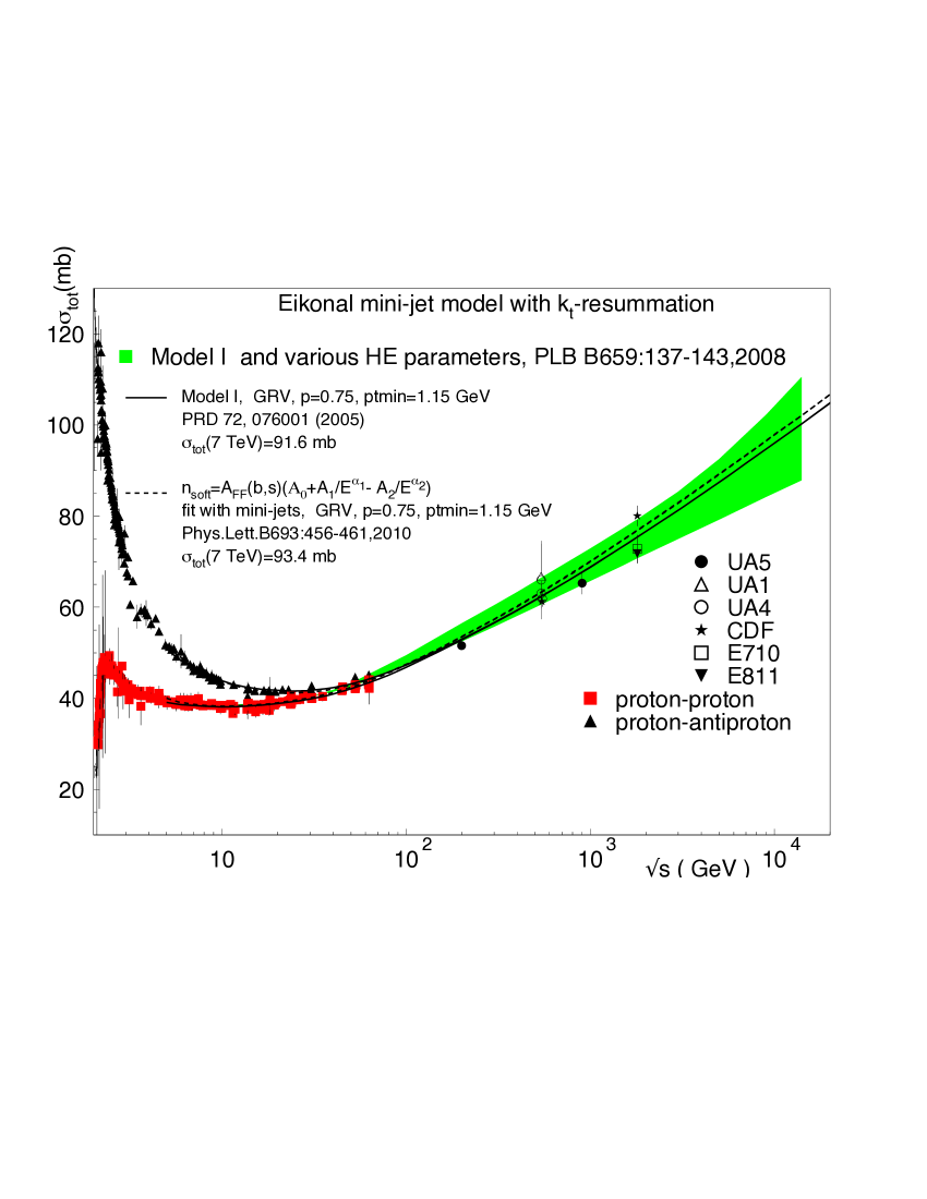
Figure 2: Total $pp$  and ${\bar{p}}p$ cross-section calculated with our model and compared with data. Values for $\sigma_{total}$ at 7 TeV at LHC are indicated.

At present LHC energies, $\sqrt{s}=7\ TeV$, we obtain $\sigma_{total}=91.6\ +6.5\ -9.7(mb)$ with Model I . The results for this model at the two LHC energies $\sqrt{s}=7,\ 14\ TeV$, are summarized in Table 1. For Model II, we have only calculated the value with GRV densities, $p_{tmin}=1.15\ GeV$, and $p=3/4$ , and the value $\sigma_{total}(\sqrt{s}=7\ TeV)=93.5\ mb$, lies within the indicated band of Model I. Our actual ignorance of a fundamental QCD description of the low energy total cross-section dynamics makes further studies of the difference between the models, quite irrelevant. However the result with low energy fits inclusive of mini-jet contribution, i.e. model II, should be preferred.

PDF	$p_{tmin}$ (GeV)	$\sigma_{0}(mb)$	p	$\sigma_{tot}$	$\sigma_{tot}$ (mb)
				$\sqrt{s}=7\ TeV$	$\sqrt{s}=14\ TeV$
GRV	1.15	48	0.75	91.6	100.3
GRV94	1.10	46	0.72	95.9	103.9
	1.10	51	0.78	83.3	89.7
GRV98	1.10	45	0.70	94.9	102.0
	1.10	50	0.77	82.1	87.8
MRST(72)	1.25	47.5	0.74	85.9	95.9
	1.25	44	0.66	97.9	110.5

Table 1: Values of $\sigma_{tot}$ for $p_{tmin}$, $\sigma_{0}$ and $p$ corresponding to different parton densities in the proton, for which our model Achilli et al. (2008) gives a satisfactory description of the total cross-section. The values are obtained with Model I (see Appendix) for ${\bar{n}}_{soft}$, the average number of soft collisions.

Having thus chosen the set of HE parameters which adequately describe the existing total cross-section data, we now proceed to investigate how the eikonal function, determined by these parameters, describes data for the inelastic cross-section.

V The inelastic proton-proton cross-section

In this section we present the results of our model for the inelastic cross-section. It is worth noting that a nontrivial bound on the inelastic cross-section, based on general analyticity arguments has been obtained only very recently Martin (2009), unlike its counterpart for the total cross-section which has been known for quite some time Froissart (1961); Martin (1963); Lukaszuk and Martin (1967).

The inelastic proton-proton cross-section is of particular interest in cosmic ray physics, as it determines the total $p-air$ cross-section Anchordoqui et al. (2004). The knowledge of this inelastic cross-section at very high energies enters the simulation of cosmic ray air showers and is used for extracting the total $pp$ cross-section from cosmic ray data. However, unlike the total and the elastic case, the inelastic cross-section is not uniquely defined and data for it suffer from usage of different cuts imposed in the analysis which lead to inlcusion of differing amounts of diffractive contribution to the measurement. In principle, the least ambiguous way to define data for the inelastic total cross-section is through the definition

$$\sigma_{inelastic}^{exp}\equiv\sigma_{total}^{exp}-\sigma_{elastic}^{exp}$$ (27)

Models can then be compared with data in the available range of energies, starting from $\sqrt{s}\simeq 1-2\ GeV$ up to the TeVatron data, and now to the LHC data at $\sqrt{s}=7\ TeV$.

As a first step towards analysing the inelastic cross-sections, one then needs to extract the values for $pp$ scattering, as the difference between the total and the elastic cross-sections. The error of this procedure is obtained by combining the errors in quadrature. Once the data points are obtained in this fashion, one can try to confront our model predictions with them. Note that there are no data for $pp$ scattering beyond the ISR energies Amsler et al. (2008). However, the increasing dominance of gluon-gluon scattering with the rising energy should allow us to use the ${\bar{p}}p$ data from CERN $S{\bar{p}}pS$ Bozzo et al. (1984) and from the TeVatron Amos et al. (1990, 1992); Abe et al. (1994a, b); Avila et al. (1999), as a guidance in our analysis. We notice that in Amos et al. (1990), in addition to the total and elastic data, the collaboration also presents a value for the inelastic cross-section at $\sqrt{s}=1800\ GeV$. There are therefore two possible values to fit, $\sigma_{total}-\sigma_{elastic}=56.2\pm 3.5\ mb$ (taking $\sigma_{tot}$ from Amos et al. (1992) and $\sigma_{el}$ from Amos et al. (1990)) or $\sigma_{inelastic}=55.5\pm 2.2\ mb$ which is the direct measure presented in Amos et al. (1990). The two values agree within the errors. In our estimate, for consistency with all the other data points, which were obtained in the same way, we use the value obtained by subtraction. For the same reason, i.e. consistency with the subtraction procedure we have outlined, we do not use results from Augier et al. (1995). Thus, in all the figures to follow, the term inelastic data corresponds to data obtained from the difference between total and elastic cross-section, as per Eq. (27) and can be directly compared with Eq. (4).

As was the case for the total cross-section, before studying the high energy behaviour, the soft part of the eikonal needs to be chosen. We shall use the Form Factor model, Model II, with two different choices for the soft cross-section $\sigma_{soft}$. In the first, Model II-A, the soft part of the eikonal, namely ${\bar{n}}_{soft}=A_{FF}\sigma_{soft}$, is the same as the one entering the total cross-section estimates shown by the dashed line in Fig 2, while in the second, Model II-O, we use an independent fit to the low energy inelastic $pp$ cross-section data with $\sqrt{s}>5$ GeV, which also includes the mini-jet contribution. As in the case of the total cross-section, at high energy, the cross-section behaviour is rather insensitive to this choice and is mainly controlled by the PDF’s and the other high energy parameters $p,p_{tmin}$.

As anticipated in Sec. II, we find that the high energy data, cannot be described by the same set of HE parameters determined from Eq.  (7) for the total cross-section, namely GRV and MRST PDFs, $p_{tmin}$ and $p$. In particular, in Fig.  3 we show a comparison between the inelastic data and the results of our model for the set of HE parameters GRV, $p_{tmin}=1.15\ GeV,p=0.75.$

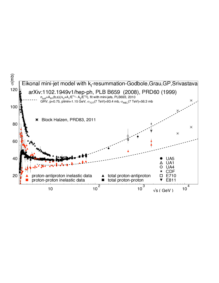
Figure 3: The total and inelastic cross-section as described by our model when using the same set of high energy parameters in the eikonal. Results are compared with pre-LHC data and an estimate from Block and Halzen (2011).

More generally, varying $p_{tmin}$ and the densities as in Table  1 within the same ranges as we did for the total cross-section, we find that the $p$-values in Table  1 always give results short of the pre-LHC data. This is consistent with the observation in Sec. II, namely that the eikonal mini-jet model with two components will only describe uncorrelated processes, while the inelastic data from Eq. (27) include also collisions in diffractive and other similarly correlated regions. On the other hand, everything else being equal, a reasonable description is obtained by letting the parameter $p$ vary between the minimum value consistent with the model Grau et al. (2009), $p=0.5$, and $0.66$, the highest value which can possibly be consistent with the total cross-section band in Achilli et al. (2008). We show this analysis in Fig. 4.

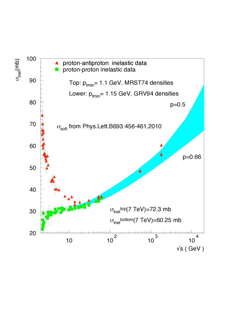
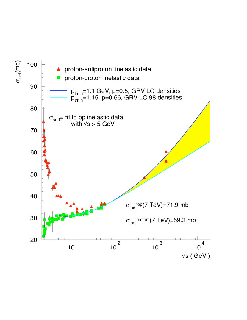
Figure 4: Predictions for the inelastic $pp$ cross-section from model II-A (left) and Model II-O (right).

We combine the results of Fig. 4 in Fig. 5. In this figure, using both Model II-A and Model II-O to constrain the low energy behaviour, we indicate all the parameter sets used to produce the bands, as well as the numerical values of interest. We see that the low energy behaviour is of course better described by Model II-O, which fits low-energy inelastic data, including mini-jets in the overall fit. However, a good description is also obtained from the same low energy eikonal entering the total cross-section (Model II-A), an indication that the two-channel eikonal model works at low energy. In this figure, for simplicity, we show the application of Model II-O only for GRV densities. Also, to compare our choice of high energy parameters with those used for the total cross-section, we have plotted a curve (black line) with same $p_{tmin}=1.15\ GeV$ and GRV densities as in Fig. 3, but with $p=0.5$, a value which we find to give a good description of the pre-LHC inelastic data.

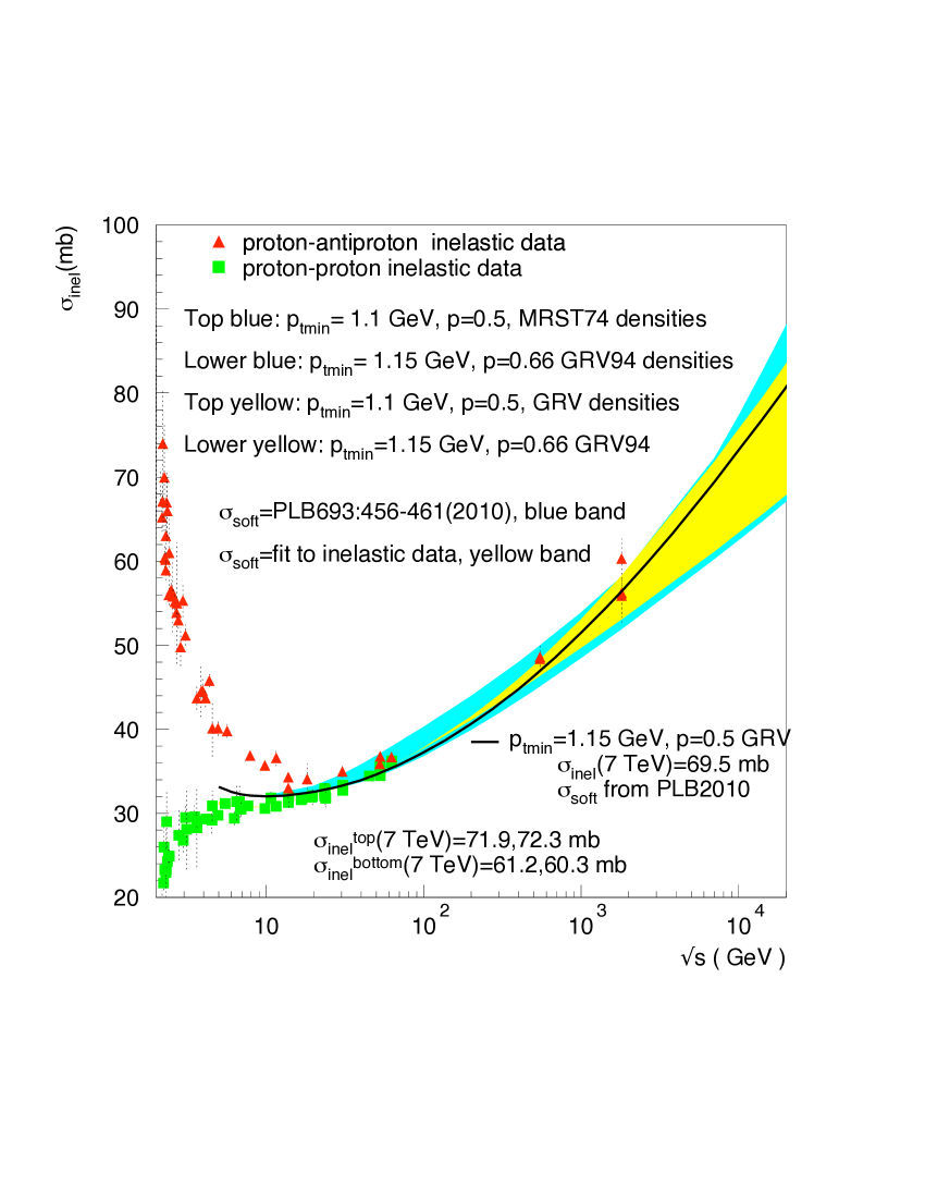
Figure 5: Comparison between data for $\sigma_{total}-\sigma_{elastic}$ with results of our model. Values for the parameters used for the band and the curve are indicated.

VI Elastic, inelastic and diffraction processes in eikonal models

In the previous section, we have seen that, up to TeVatron energies, the two channel model cannot accomodate both inelastic (diffraction included) and total cross-section data without a change of parameters. On the other hand by changing the singularity parameter $p$, in a way consistent with our understanding of the role played by the parameter, the model results can span both the total and the inelastic data at energies up to the TeVatron (blue band). We shall now combine the results of our eikonal mini-jet model for the total and the inelastic cross-section in a single figure and compare the latter with ATLAS recent results Aad et al. (2011) and with a recent calculation by Block and Halzen Block and Halzen (2011). In Fig. 6 the upper (green) band is from Fig. 2 and the lower (blue) band from Fig. 5 . Once a set of parameters has been fixed from the total cross-section data, the dashed curves indicate what the two-channel eikonal mini-jet model would predict, without changing any parameter in going from the total to the inelastic. As already mentioned, the dashed curve for the inelastic cross-section does not fit the TeVatron data, nor the $S{\bar{p}}pS$ data, but its comparison with the recently released ATLAS measurement or preliminary CMS data in the central region can be very instructive. The dashed line (see Fig. 3), corresponding to the model with the same $p$ value as in the total cross-section curves, is close to the preliminary value reported by the CMS Collaboration for inelastic events with at least 2 charged particles with $\eta<2.4$ and $p_{\perp}>200MeV/c^{2}$ cms (2011) This confirms the interpretation of the two-channel eikonal minijet model, put forward in Sect. II, namely that this model describes total inelastic processes, with little or no correlations.

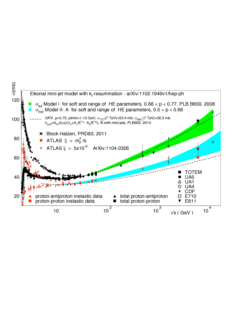
Figure 6: Total and inelastic data for $pp$ and ${\bar{p}}p$ scattering compared with the prediction from our model (dashed curve)Achilli et al. (2011), in the two-channel case, when the same eikonal function is used both for the total and the inelastic cross-sections, from low to high energy. The upper band is the same as in Fig.2, the lower band for the inelastic cross-section is the same as in the left panel of Fig. 4. Comparison is made with theoretical predictions by Block and Halzen Block and Halzen (2011), with TOTEM data Latino et al. (2011) for the total cross-section, ATLAS inelastic data extrapolated to $\xi>m^{2}_{p}/s$ and with ATLAS data in the range $5\times 10^{-6}$, where $\xi=M^{2}_{X}/s$ (star symbol) Aad et al. (2011).

On the other hand, with the present parametrization, but changing the parameter $p$, we find that our lower (blue) band is consistent with the ATLAS results, as corrected for diffraction Aad et al. (2011) (full circle).

Let us now discuss the missing element in Eq. (4), that is a category of processes which are inelastic but correlated, namely single and double diffraction. In diffraction, partons in the final state resulting from multiple collisions or from soft gluon emission must recombine into a proton or are constrained to be emitted along the outgoing proton. It would then be more correct to write Eq.( 6) as

$$\sigma_{inel}^{uncorrelated}(s)=\sum_{n=1}\int d^{2}{\bf b}\ P(\{n,{\bar{n}}\})=\int d^{2}{\bf b}[1-e^{-{\bar{n}}(b,s)}]$$ (28)

so that, generally speaking,

$$\sigma_{total}=\sigma_{elastic}+\sigma_{inel}^{diff}+\sigma_{inel}^{uncorrelated}$$ (29)

and include in $\sigma_{inel}^{diff}$ all correlated processes, like single and double diffraction. Thus Eq.  (4) can be used only for inelastic uncorrelated processes, while the inelastic correlated processes are to be described separately.

On the other hand, the above considerations do not yet suggest how to include the diffractive processes. The solution adopted in this paper, illustrated by the lower (blue) band in Fig. 6, has been to mimick the presence of diffraction processes using different values for the singularity parameter $p$ in Eqs.  (6) and (7). By comparing with previous data, Figs. 5 and 6 indicate that the value $p=0.5$, with the present LO parameterization (LO GRV and MRST), gives the best description of the total inelastic cross-section, while the above discussion, following the one in in Sec. II, indicates that values with $p=0.75$ would only include uncorrelated inelastic processes.

For the future, once the parameters of the model have been tuned to the measured total cross-section, more precise predictions for the totality of uncorrelated inelastic events could be extracted from our model.

VI.1 Uncertainties and the nature of the theoretical band

For clarity and completeness, we recapitulate here the uncertainties in our model and the nature of the bands we have presented. The bands in this paper preceded the release of LHC data for total and inelastic cross-sections, and reflect how well the model worked in describing lower energy data Godbole et al. (2008); Achilli et al. (2011) as well as their uncertainties, mostly the TeVatron data for the total cross-section. For the future, the new data will allow a better tuning of all the parameters involved and hence firmer predictions for total cross-section data at ultra high energies or for quantities, such as survival probabilities, needing the inelastc cross-section.

Even so, the bands we have presented are in reasonable agreement with the new data and provide confirmation of our understanding of the eikonal two-channel model. The blue (lower ) band in Fig.  6 describes the interplay between all the HE energy parameters. The essential parameters are the PDFs, $p_{tmin}$ and $p$. The PDFs control both the rise (mini-jets) as well as the logarithmic asymptotic behavior through $q_{max}$. At fixed $p_{tmin}$, different PDF’s lead to different values for $\sigma_{jet}$ and for $q_{max}$. In the present formulation, $\sigma_{jet}$ are controlled by uncertainties in the LO low-$x$ behaviour of the gluon densities, and $q_{max}$ by the LO valence quark densities. The lower is $p_{tmin}$ the faster the rise, and, at high energies, the more this rise needs to be quenched. The quenching of the rise depends on how much is the allowed loss in transverse momentum, $q_{max}$ and upon the degree of singularity of the effective coupling, the parameter $p$, for which we have both an upper as well as a lower bound. For the convergence of the IR integrals, it is incumbent that $p<1$. [It must be recalled that the Wilson equal area rule leading to a strictly linear potential viz., $p=1$ is not allowed in our resummed model]. On the other hand, it is easy to check that there is no confining potential if $p<1/2$.

Within the contraint $1/2<p<1$, values for this parameter are determined through the phenomenological description of the data. There is an interesting interplay between the phenomenological value of $p$ and its weight in describing the uncorrelated versus correlated events. In the model, once the value for $p$ has been fixed through the total cross-section, it can be used to describes the uncorrelated inelastic events, while the fully inelastic data need a different treatment. We have mimicked the amount of diffraction to include in the full inelastic cross-section by decreasing values of $p$. As $p$ is decreased, the amount of acollinearity introduced by the soft-gluon radiation changes. We see, that a description of the underlying fully inelastic data would favour $p=0.5$.

Finally, we point out that some uncertainties are also introduced by the different purely phenomenological models for the quantity ${\bar{n}}_{soft}$ and are reflected in the band for the inelastic cross-section.

VII Conclusions

We have presented results from the two channel eikonal model for the inelastic cross-section. We have shown that such formulation only describes uncorrelated processes, a result independent of the details of the model used to describe the data. This observation clarifies the origin of a long standing difficulty of the two channel eikonal models well known to people working in total and inelastic cross-sections.

We have shown numerical results for the description of total and inelastic cross-sections at LHC at $\sqrt{s}=7\ TeV$ and beyond, using our QCD based model. Our numerical results are obtained in a LO QCD model for collisions, embedded in the eikonal formulation. The major QCD phenomenological input is from Parton Density Functions, which can be considered QCD parameters through which we build our eikonal in order to describe the two high energy effects: the rise at the beginning and the slowing down towards asymptotia. While it is difficult to describe these two effects in QCD models which satisfy unitarity and the Froissart bound, in our model we have both.

We have found that with exactly the same low energy parameters entering the total cross-section calculation, but with different values of the high energy parameters $p$ and $p_{tmin}$, our model predictions catch the TeVatron data as well as new data from the ATLAS collaboration Aad et al. (2011). On the other hand, if no parameters are changed at all in the eikonal function used for $\sigma_{total}$, our results agree with the hypothesis that the simple two-channel eikonal mini-jet models describe only the non-diffractive part of the inelastic cross-section. We defer to future work an analysis of the inelastic cross-section which might include correlations in the diffractive terms, or inclusion of a non zero $\Re e\chi(b,s)$.

Appendix A The average number of soft collisions ${\bar{n}}_{soft}(b,s)$

As in the case of the hard collisions, we approximate ${\bar{n}}_{soft}(b,s)$ with the factorized expression

$${\bar{n}}_{soft}(b,s)=A_{soft}(b,s)\sigma_{soft}(s)$$ (30)

and then use two different phenomenological parametrizations for the average number of soft collisions. In the first model, Model I, we assume that the decrease in the proton proton total cross-section is due only to soft gluon emission.

A.0.1 Model I, $A_{soft}(b,s)$ given by resummation expression:

This is the model adopted in our analyses in Refs.  Godbole et al. (2005); Achilli et al. (2008). In this case, for the $b$-distribution, we use Eq. (16), i.e. the BN model. In this equation, we parametrize $q_{max}$ to make it vary slowly with energy, thus giving a slight (decreasing) energy dependence to $A_{soft}(b,s)$ Godbole et al. (2005). In Table  2 from Godbole et al. (2005) we reproduce the values of $q_{max}^{soft}$ used to evaluate $A_{soft}(b,s)$. These values correspond to the observation that for processes contributing to $n_{soft}$, a soft gluon will always carry away less energy than for those contributing to $n_{hard}$. The question is how much lower is the allowed energy. The above set of values is purely phenomenological and the values are those we found to give an acceptable description for $\sigma_{pp}$ before the rise.

Table 2: Average $q_{max}$ values used for the impact parameter distribution of the soft part of the eikonal

$\sqrt{s}(GeV)$	$q_{max}^{soft}(GeV)$
5.	0.19
6.	0.21
7.	0.22
8.	0.23
9.	0.235
10.	0.24
50.	0.24
100	0.24

For $pp$ scattering, where the s-channel is exotic and no trajectories are exchanged in the $t-$channel, our use of soft gluon emission using a form for $A_{BN}(b,s)$ a-la Eq. (16) with $q_{max}$ chosen as explained above, is sufficient to explain the slight decrease at low energies, in the total $pp$ cross-section. The situation is more complicated for ${\bar{p}}p$. As described in  Godbole et al. (2005), we then simply write for the cross-section

$$\sigma_{soft}(s)=\sigma_{0}[1+\frac{2\epsilon}{\sqrt{s}}]$$ (31)

with $\sigma_{0}$ a constant, as in Table  1 and $\epsilon=0,1$ for $pp$ and ${\bar{p}}p$ respectively.

A.0.2 Model II, $A_{soft}(b,s)$ given by $A_{FF}(b,s)$:

In the second approach, for the soft collisions we have used the Form Factor model for $A(b,s)$, Eq.(12),together with a standard, Regge exchange inspired parametrization of ${\bar{p}}p$  and $pp$ cross-sections at low energy, namely

$$\sigma_{soft}(s)=\sigma_{0}+\frac{A_{1}}{(E_{lab})^{\alpha_{1}}}\mp\frac{A_{2}}{(E_{lab})^{\alpha_{2}}}$$ (32)

with $\mp$ referring to $pp$ and ${\bar{p}}p$ respectively, and the constant parameters determined through a fit to the low energy data. In earlier publications, such as Ref. Grau et al. (1999), the fit to low energy data was done using an expression which did not include the mini-jet contribution, whereas in our more recent analysis Grau et al. (2010) the minijet contribution is included in the fit. From the point of view of the $\chi^{2}$, the difference in the results is not noticeable. In Table 3 from Grau et al. (2010) we reproduce the values of various parameters used in Eq.  (32).

Table 3: Results of the fit to $pp$ and ${\bar{p}}p$ data.

Fit for $pp$	Fit for ${\bar{p}}p$
$\sigma_{0}=(48.20\pm 0.19)$ mb	$\sigma_{0}=(47.86\pm 2.47)$ mb
$A_{1}=101.66\pm 16.35$    $\alpha_{1}=0.99\pm 0.13$	$A_{1}=132.07\pm 32.89$       $\alpha_{1}=0.69\pm 0.14$
$A_{2}=27.89\pm 4.78$    $\alpha_{2}=0.59\pm 0.04$	$A_{2}=0.82\pm 0.31$       $\alpha_{2}=0.52\pm 0.07$
$\chi^{2}=154.1/(102+5-1)$	$\chi^{2}=24.65/(31+5-1)$

References

- Heisenberg (1952) W. Heisenberg, Z. Phys. 133, 65 (1952).
- Aad et al. (2011) G. Aad et al. (ATLAS Collaboration) (2011), * Temporary entry *, eprint 1104.0326.
- cms (2011) CMS-PAS-FWD-11-001 (2011), preliminary CMS results.
- Achilli et al. (2011) A. Achilli et al. (2011), eprint 1102.1949.
- Block and Halzen (2011) M. M. Block and F. Halzen, Phys.Rev. D83, 077901 (2011), eprint 1102.3163.
- Goulianos (2011) K. Goulianos (2011), * Temporary entry *, eprint 1105.4916.
- Jenkovszky et al. (2011) L. Jenkovszky, A. Lengyel, and D. Lontkovskyi (2011), * Temporary entry *, eprint 1105.1202.
- Latino et al. (2011) G. Latino, G. Antchev, P. Aspell, I. Atanassov, V. Avati, J. Baechler, V. Berardi, M. Berretti, E. Bossini, M. Bozzo, et al. (2011), eprint arXiv/1110.1008.
- Abreu et al. (2011) P. Abreu et al. (The Pierre Auger Collaboration) (2011), * Temporary entry *, eprint 1107.4804.
- Corsetti et al. (1996) A. Corsetti, A. Grau, G. Pancheri, and Y. N. Srivastava, Phys. Lett. B382, 282 (1996), eprint hep-ph/9605314.
- Grau et al. (1999) A. Grau, G. Pancheri, and Y. Srivastava, Phys.Rev. D60, 114020 (1999), eprint hep-ph/9905228.
- Godbole et al. (2005) R. M. Godbole, A. Grau, G. Pancheri, and Y. N. Srivastava, Phys. Rev. D72, 076001 (2005), eprint hep-ph/0408355.
- Glauber (1959) R. J. Glauber, High energy collision theory (Interscience Publishers Inc., New York, 1959), in Lectures in Theoretical Physics, Vol. I, Boulder 1958.
- Glauber and Matthiae (1970) R. J. Glauber and G. Matthiae, Nucl. Phys. B21, 135 (1970).
- Cline et al. (1973) D. Cline, F. Halzen, and J. Luthe, Phys. Rev. Lett. 31, 491 (1973).
- Gaisser and Halzen (1985) T. K. Gaisser and F. Halzen, Phys. Rev. Lett. 54, 1754 (1985).
- Pancheri and Srivastava (1986) G. Pancheri and Y. N. Srivastava, Phys. Lett. B182, 199 (1986).
- Durand and Hong (1987) L. Durand and P. Hong, Phys. Rev. Lett. 58, 303 (1987).
- Durand and Pi (1989) L. Durand and H. Pi, Phys. Rev. D40, 1436 (1989).
- Durand and Pi (1988) L. Durand and H. Pi, Phys. Rev. D38, 78 (1988).
- Margolis et al. (1988) B. Margolis, P. Valin, M. M. Block, F. Halzen, and R. S. Fletcher, Phys. Lett. B213, 221 (1988).
- Fletcher et al. (1992) R. S. Fletcher, T. K. Gaisser, and F. Halzen, Phys. Rev. D45, 377 (1992).
- Honjo et al. (1993) K. Honjo, L. Durand, R. Gandhi, H. Pi, and I. Sarcevic, Phys. Rev. D48, 1048 (1993), eprint hep-ph/9212298.
- Block et al. (1999) M. M. Block, E. M. Gregores, F. Halzen, and G. Pancheri, Phys. Rev. D60, 054024 (1999), eprint hep-ph/9809403.
- Block et al. (2000) M. M. Block, F. Halzen, and T. Stanev, Phys. Rev. D62, 077501 (2000), eprint hep-ph/0004232.
- Godbole et al. (2006) R. M. Godbole, A. Grau, R. Hegde, G. Pancheri, and Y. Srivastava, Pramana 66, 657 (2006), eprint hep-ph/0604214.
- Achilli et al. (2008) A. Achilli et al., Phys. Lett. B659, 137 (2008), eprint 0708.3626.
- Grau et al. (2010) A. Grau, G. Pancheri, O. Shekhovtsova, and Y. N. Srivastava, Phys.Lett. B693, 456 (2010), eprint 1008.4119.
- Godbole et al. (2009) R. Godbole, A. Grau, G. Pancheri, and Y. Srivastava, Eur.Phys.J. C63, 69 (2009), eprint 0812.1065.
- Godbole and Pancheri (2001) R. M. Godbole and G. Pancheri, Eur. Phys. J. C19, 129 (2001), eprint hep-ph/0010104.
- Godbole et al. (2008) R. M. Godbole, A. Grau, G. Pancheri, and Y. N. Srivastava, Nucl. Phys. Proc. Suppl. 184, 85 (2008), eprint 0802.3367.
- Lipari and Lusignoli (2009) P. Lipari and M. Lusignoli, Phys. Rev. D80, 074014 (2009), eprint 0908.0495.
- Anchordoqui et al. (2004) L. Anchordoqui et al., Ann. Phys. 314, 145 (2004), eprint hep-ph/0407020.
- Bjorken (1993) J. Bjorken, Phys.Rev. D47, 101 (1993).
- Block and Halzen (2001) M. Block and F. Halzen, Phys.Rev. D63, 114004 (2001), eprint hep-ph/0101022.
- Bloch and Nordsieck (1937) F. Bloch and A. Nordsieck, Phys.Rev. 52, 54 (1937).
- Pancheri-Srivastava and Srivastava (1977) G. Pancheri-Srivastava and Y. Srivastava, Phys. Rev. D15, 2915 (1977).
- Dokshitzer et al. (1978) Y. L. Dokshitzer, D. Diakonov, and S. I. Troian, Phys. Lett. B79, 269 (1978).
- Parisi and Petronzio (1979) G. Parisi and R. Petronzio, Nucl. Phys. B154, 427 (1979).
- Sudakov (1956) V. V. Sudakov, Sov. Phys. JETP 3, 65 (1956).
- Nakamura et al. (1984) A. Nakamura, G. Pancheri, and Y. Srivastava, Z.Phys. C21, 243 (1984).
- Grau et al. (2009) A. Grau, R. M. Godbole, G. Pancheri, and Y. N. Srivastava, Phys.Lett. B682, 55 (2009), eprint 0908.1426.
- Chiappetta and Greco (1981) P. Chiappetta and M. Greco, Phys. Lett. B106, 219 (1981).
- Dokshitzer (1998) Y. L. Dokshitzer (1998), eprint hep-ph/9812252.
- Dokshitzer et al. (1999) Y. L. Dokshitzer, G. Marchesini, and B. Webber, JHEP 9907, 012 (1999), eprint hep-ph/9905339.
- Gluck et al. (1992) M. Gluck, E. Reya, and A. Vogt, Z. Phys. C53, 127 (1992).
- Sherstnev and Thorne (2008) A. Sherstnev and R. S. Thorne, Eur. Phys. J. C55, 553 (2008), eprint 0711.2473.
- Pancheri et al. (2007) G. Pancheri, R. Godbole, A. Grau, and Y. Srivastava, Acta Phys. Polon. B38, 2979 (2007), eprint hep-ph/0703174.
- Gluck et al. (1995) M. Gluck, E. Reya, and A. Vogt, Z. Phys. C67, 433 (1995).
- Gluck et al. (1998) M. Gluck, E. Reya, and A. Vogt, Eur. Phys. J. C5, 461 (1998), eprint hep-ph/9806404.
- Martin et al. (1998) A. D. Martin, R. G. Roberts, W. J. Stirling, and R. S. Thorne, Eur. Phys. J. C4, 463 (1998), eprint hep-ph/9803445.
- Martin (2009) A. Martin, Phys. Rev. D80, 065013 (2009), eprint 0904.3724.
- Froissart (1961) M. Froissart, Phys. Rev. 123, 1053 (1961).
- Martin (1963) A. Martin, Phys. Rev. 129, 1432 (1963).
- Lukaszuk and Martin (1967) L. Lukaszuk and A. Martin, Nuovo Cim. A52, 122 (1967).
- Amsler et al. (2008) C. Amsler et al. (Particle Data Group), Phys. Lett. B667, 1 (2008).
- Bozzo et al. (1984) M. Bozzo et al. (UA4), Phys. Lett. B147, 392 (1984).
- Amos et al. (1990) N. A. Amos et al. (E-710), Phys. Lett. B243, 158 (1990).
- Amos et al. (1992) N. Amos et al. (E710), Phys. Rev. Lett. 68, 2433 (1992).
- Abe et al. (1994a) F. Abe et al. (CDF), Phys. Rev. D50, 5518 (1994a).
- Abe et al. (1994b) F. Abe et al. (CDF), Phys. Rev. D50, 5550 (1994b).
- Avila et al. (1999) C. Avila et al. (E811), Phys. Lett. B445, 419 (1999).
- Augier et al. (1995) C. Augier et al. (UA4/2), Phys. Lett. B344, 451 (1995).