Viscoelastic flow transitions in abrupt planar contractions

ABSTRACT

We present experimental evidence of global viscoelastic flow transitions in 2:1, 8:1 and 32:1 planar contractions under inertia-less conditions. Light sheet visualization and laser Doppler velocimetry techniques are used to probe spatial structure and time scales associated with the onset of these instabilities. The results are reported in terms of critical Weissenberg numbers characterizing the fluid flow rates. For a given contraction ratio and polymer fluid, a two-dimensional, steady flow with converging streamlines transitions to a two-dimensional pattern with diverging streamlines beyond a critical Weissenberg number. At even higher Weissenberg numbers, spatial transition to three-dimensional flow is observed. A relationship between the upstream Weissenberg number for the onset of this spatial instability and the contraction ratio is derived. For contraction ratios substantially greater than unity, we observe that further increase in the flow rate results in a second temporal transition to a three-dimensional, time-dependent flow. This complex flow arises due to a combination of the effects of stress-curvature interaction and three dimensional perturbations induced by the walls bounding the neutral direction. Comparison with studies on other geometries indicates that boundary shapes deeply influence the sequence and nature of flow transitions.

Keywords Viscoelastic flow transitions, planar contraction flow, critical Weissenberg number

I Introduction

A common and important class of flows is constituted by the motion of a polymer liquid through abrupt planar and axisymmetric contraction geometries. These flows also constitute canonical benchmarks to test numerical codes and hence have been a subject of a few experimental studies. In this article, we describe detailed experimental studies on viscoelastic flow transitions in 2:1, 3:1 and 32:1 planar contraction geometries. A novel Boger fluid that allows us to obtain flows with negligible inertial effects is used as the test fluid, thus the instabilities are purely due to fluid elasticity. Our focus is on the classification of global flow transitions in the planar contraction, i.e., those which occur over the longest characteristic length scale of the geometry which is the upstream half-height. The flow transitions are characterized via a suitably defined aspect ratio that captures the effects of flow geometry, and the Weissenberg number ($We=\lambda/t_{\mathrm{def}}$), $\lambda$ being a characteristic relaxation time of the viscoelastic fluid and $t_{\mathrm{def}}$ a characteristic measure of the local deformation time scale (an inverse strain rate) respectively.

Previous investigations of complex flow through diverse geometries [1-13] have revealed transitions in the flow structure associated with viscoelastic effects as the flow rate is varied. Binding and Walters [2] used a polyacrylamide-based Boger fluid in studies on flows through a 14:1 planar contraction at flow conditions for which inertial effects were in-significant. At high flow rates, a two-dimensional rearrangement of the flow field to a pattern of diverging streamlines occurred upstream of the contraction plane. This pattern was also observed in flow experiments by Evans and Walters [3] of a polyacrylamide solution through a 4:1 contraction under conditions where inertial effects could not be neglected. Chiba et al. [4,6] used non-dilute shear-thinning, aqueous polyacrylamide solutions flowing through planar contractions. For contraction ratios of 3.3:1 and 5:1 but not for the 10:1 contraction, the onset of diverging flow was seen at a critical flow rate. As in the Evans and Walters study, inertia was a significant factor. Similar rearrangement of the flow is observed for viscoelastic flows through axisymmetric contraction geometries. Experiments indicate that lower contraction ratio geometries in both the planar and axisymmetric contractions result in more pronounced diverging flow behavior than higher contraction ratio configurations. The maximum contraction ratio for which diverging flow is observed is also typically greater for planar than for axisymmetric contraction flows

Transitions from a two-dimensional base flow to three-dimensional steady or time-dependent flow have also been observed in flow through abrupt contractions and also in flows through other geometries. Work by Binding and Walters [2] revealed transition to an asymmetry in the velocity field at a critical $We$ greater than that associated with the transition to diverging flow streamlines. The spatial structure of the post-transition flow comprised of vortical structures. Experiments by Chiba et al. [4,6] in 3.3:1 and 10:1 contractions also revealed a transition from two- to three-dimensional flows at flow rates above that required for the onset of diverging flow. The spatial structure of the flow in these experiments also was found to consist of interlaced pairs of counter-rotating vortices on each side of the center-plane. At yet higher flow rates, a transition was seen from the three-dimensional, steady flow to three-dimensional, time-dependent flow. It was difficult to identify unambiguously the mechanism driving the flow transition, as inertial effects were significant at the flow rates attained.

In general velocity-field transition sequences for a variety of complex flows are evidenced to share a number of common features. For a given contraction ratio we expect the rheology of the polymer fluid and elongational flow material functions to influence the evolution of the velocity field. In all cases for which a two-dimensional flow rearrangement occurred, the critical $We$ was lower than the value of $We$ characterizing transition to three-dimensional and/or time-dependent flow. The spatial structure of the flow after transition had the form of Görtler-type vortices. However, there are also significant differences. In some geometries, a direct transition from a two-dimensional, steady flow to a three-dimensional, time-dependent flow was observed; flows through other geometries first undergo a spatial transition to three-dimensional flow and then a temporal transition to time-dependent flow.

In the following sections, we report on extensive experimental results on the structure of the viscoelastic flow transitions in planar contraction flow where both contraction ratio and the flow rate characterized by a typical Weissenberg number are varied. Light sheet visualization coupled with laser Doppler velocimetry (LDV) measurements is used to characterize quantitatively the critical Weissenberg numbers, length, and time scales associated with the onset of the instabilities. Scaling based on the viscoelastic Görtler number analysis complemented by plots of appropriate measures of the velocity patterns are used to construct transition and bifurcation maps. Finally, the flow structures observed in planar contraction flows are compared with those identified in other flow geometries.

II Experimental test geometry and fluid handling system

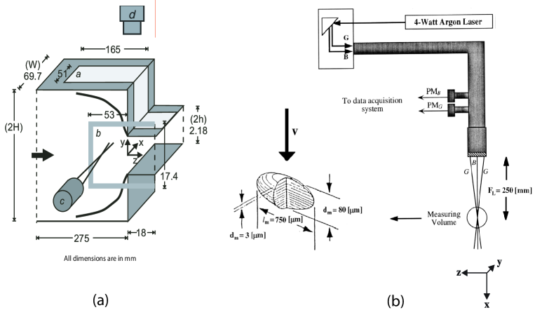
Figure 1: (A) Planar contraction test geometry. Fixed dimensions of the geometry, $W$ and $2h$, and the dimensions of the windows are shown; the upstream channel height, $2H$ is variable. (a) Top window for flow visualization in the x-z plane, (b) The side window, constructed of SF-57 glass, is used for LDV and FIB measurements. (c) The final focusing optics from which the dual beams of the LDV system emanate are illustrated; the FIB probe beam is not shown and (d) video camera for recording images in the x-z plane (light sheet). All dimensions are in millimeters. (B) Schematic diagram of the two-component LDV system used in this study and the measuring volume.

The planar contraction test geometry used in this study is illustrated in Figure 1(A). The exterior of the geometry was constructed of anodized aluminum. Fluid flowed in the $z$-direction from an upstream duct of half-height $H$ into a smaller, downstream duct of half-height $h$. The width, $W$, is fixed throughout the geometry. A downstream insert constructed of anodized aluminum and borosilicate glass (BK-10, Schott Glass Technologies) was used to set the half-height of the downstream slit, $h=1.09$$\pm$ $0.05$ mm. The contraction ratio, $H/h$, was varied by changing the upstream insert also constructed of anodized aluminum and polymethylmethacrylate (PMMA). Qualitative, full-field streakline observations of the kinematic structure of the flow in the $xz$-plane were made through windows placed in the top of the geometry, $a$. Quantitative LDV measurements of the $v_{y}$ or $v_{z}$ velocity component and full field streakline observations of flow in the $yz$-plane were made through a window placed in the side of the contraction geometry, $b$. The FIB measurements also were conducted through the window, $b$. To minimize the influence of parasitic birefringence on the FIB measurement, the window was constructed of SF-57 glass (Schott Glass Technologies); this material has a low stress optical coefficient of C = 0.02 $\times$ 10^-12 Pa^-1 at 589 nm. The faces of the glass were polished and coated to minimize reflections. The fluid was driven in batch mode by nitrogen pressure from a supply tank through the test cell and into a receiving tank maintained at atmospheric pressure with the fluid flow rate adjusted by controlling the gas pressure with a self-relieving regulator.

The coordinate system used throughout this paper is as indicated in Figure 1(A). The origin is located in the center of the downstream duct, at the contraction plane ($z=0$, where the upstream and downstream ducts join). The dimensional coordinates $(x,y,z)$ are given in millimeters; dimensionless coordinates are based on the downstream half-height: $\chi=x/h$, $\upsilon=y/h$, and $\zeta=z/h$. The term center-plane refers to the plane defined by $(\chi,\upsilon=0,\zeta)$; centerline refers to any line in this plane with a constant value of $\chi$. Because the geometry is nominally two-dimensional, $x$ is referred to as the neutral direction. The width $W$ of the geometry was held constant at 69.8 mm, so that in the upstream region, a truly two-dimensional flow was most closely approximated for low contraction ratios. For the $H/h$ = 32 contraction ratio, the upstream aspect ratio was only $W/2H$ = 1.

The light sheet visualization technique was used to record a streakline image of the velocity field in a selected two-dimensional plane. A laser beam is passed through a cylindrical lens to form a light sheet with thickness of approximately 100 $\mu m$ throughout the illuminated region of the flow field. As the particles in the fluid travel through the sheet they scatter light which is recorded by a video camera; the axis of the video camera is normal to the light sheet. Two configurations were used in the experiments: in the first the light sheet was formed in the $xz$-plane to acquire a top view. In the second the light sheet was formed in the $yz$-plane to acquire a side view. The video camera signal was stored and subsequently digitized using a frame grabber board. Frames in a time series were superimposed and averaged using image processing software (NIH Image v. 1.55). By averaging together several frames separated by equal intervals of time streak-line images were produced. The length and direction of a given streak corresponded to the local velocity vector in the plane of the light sheet. To visualize the three-dimensional spatial structure of the instability, images were acquired for a given flow with light sheets in the $xz$-plane at several $y$-positions and in the $yz$-plane at various $x$-positions. These sets of two-dimensional images were used to construct a three-dimensional schematic picture of the flow field.

The specific configuration of the LDV system (TSI, Model 9100-12) used is illustrated in Figure 1(B). The output of a 4 Watt multi-line argon-ion laser is passed through a series of optical elements and a final focusing lens of focal length F_L = 250 mm to form two pairs of intersecting beams orthogonal to each other and capable of measuring the $v_{y}$ (blue beam pair) and $v_{z}$ (green beam pair) velocity components. The half-angle included by each beam pair is 0.083 rad; the half-angle in conjunction with the wavelength sets the fringe spacing $d_{f}$ = 3.1 $\mu$m. The superimposed measuring volumes from the two beam pairs are ellipsoids with dimension 80 $\mu$m $\times$ 80 $\mu$m $\times$ 500 $\mu$m in air, the long axis positioned along the x-direction (in the 0.30 wt% PIB in PB test fluid, which has a relative refractive index of 1.50, the dimensions of the measuring volume are approximately 80 x 80 x 750 $\mu$m). The LDV optics are mounted on a three axis translating table (TSI, Model 9500) capable of positioning the measuring volume to within $\pm$ 4 $\mu$m.

Under steady flow conditions, velocity data is collected by operating the system in the spectrum analysis mode. The Doppler burst signals detected by the photomultiplier (PM) tube are passed through an FFT spectrum analyzer (Nicolet, Model 660B) which calculates the power spectrum (PS). The velocity of the particles passing through the measuring volume is then determined from the characteristic frequency of the peak in the PS. The PS of a number of successive bursts is averaged together to enable accurate measurement of low velocities. For time-dependent flows, we use a frequency tracker (DISA, Model 55N20/21) to follow the Doppler frequency. To ensure adequate data collection rate, the fluid was seeded with 2 $\mu$m silicon carbide scattering particles (TSI 10081); a seeding density of 0.036 g/l was used. This ameliorated the problem of tracker drop out.

III Determination of fluid properties

The two-component experimental test fluid consisted of a homogeneous mixture of high molecular weight polyisobutylene (PIB) (Exxon Vistanex L120), with molecular weight of $M_{w}$ $=2$ $\times$ 10⁶ gmol^-1, and polybutene (PB) (Amoco Panalane H300E), with $M_{w}$ $\approx 1.3$ $\times$ 10³ gmol^-1. The fluid was produced by first dissolving polyisobutylene in chromatography grade hexane to a concentration of 2 wt %; this solution was then combined with PB. The hexane was evaporated under nitrogen purge and then under vacuum at 70C from the PIB/PB/hexane mixture to obtain the 0.30 wt% PIB in PB solution. The two-component Boger test fluid did not exhibit beam divergence when sheared in a Couette cell.

In order to interpret the experimental data, we considered both the four-mode linear Maxwell model and the four-mode non-linear Giesekus model. The generalized linear Maxwell model was used to interpret the linear viscoelastic spectrum of the fluid whereas the Giesekus model was used to characterize the shear thinning occurring at finite strains. The multi mode formulation yields the total stress tensor, $\tau$,

$${\mbox{\boldmath$\tau$}}(t)=\sum_{k=1}^{N_{\mathrm{modes}}}\mbox{\boldmath$\tau$}_{k}(t)+\mbox{\boldmath$\tau$}_{s}=\sum_{k=1}^{N_{\mathrm{modes}}}\mbox{\boldmath$\tau$}_{k}(t)-\eta_{s}\dot{\mbox{\boldmath$\gamma$}}$$ (1)

as a linear superposition of the components associated with the $k$-th mode of the relaxation spectrum. Since the PB solvent exhibits a Newtonian response on the time scale and for the stress levels attained in these experiments, we include the contribution of a Newtonian solvent to the total stress in Equation (1). Linear viscoelasticity is characterized using the generalized linear Maxwell model for which the $k$-th mode can be written as

$$\mbox{\boldmath$\tau$}_{k}+\lambda_{k}{{\partial{\mbox{\boldmath$\tau$}_{k}}\over\partial{t}}}=-\eta_{k}\dot{\mbox{\boldmath$\gamma$}}$$

where $\dot{\mbox{\boldmath$\gamma$}}$ is the strain-rate tensor, $\lambda_{k}$, the relaxation time, $\eta_{k}$, the viscosity, and $t$, the time. To describe the shear-thinning nature of the fluid, we use the non-linear Giesekus model with the $k$-th mode stress contribution given by

$$\mbox{\boldmath$\tau$}_{k}+\lambda_{k}({\mbox{\boldmath$\tau$}_{k}})_{1}-\alpha_{k}{\lambda_{k}\over\eta_{k}}(\mbox{\boldmath$\tau$}_{k}\boldsymbol{\cdot}\mbox{\boldmath$\tau$}_{k})=-\eta_{k}\dot{\mbox{\boldmath$\gamma$}}.$$

The temperature dependence of the material functions for the 0.30 wt% PIB in PB test fluid was determined by measuring the dynamic viscosity of a fluid sample undergoing oscillatory shear in a cone-and-plate configuration and sweeping the temperature over a range from 15C to 35C. An Arrhenius expression was used to estimate the temperature dependence for the test fluid and pure solvent. The rheology of the polybutene solvent was characterized in a RMS-800 mechanical spectrometer. No decreasing trend in the dynamic viscosity with increasing frequency was discerned up to $\omega_{\mathrm{max}}=100$ s^-1, the value up to this frequency being $\eta^{\prime}_{s}=79$ Pa s. This compared very well well with the viscosity of the polybutene measured in steady-shear flow, $\eta_{s}$ up to a shear rate of 26 s^-1. At greater shear rates a gradual decrease in the viscosity with shear rate is apparent; this was attributed to viscous heating.

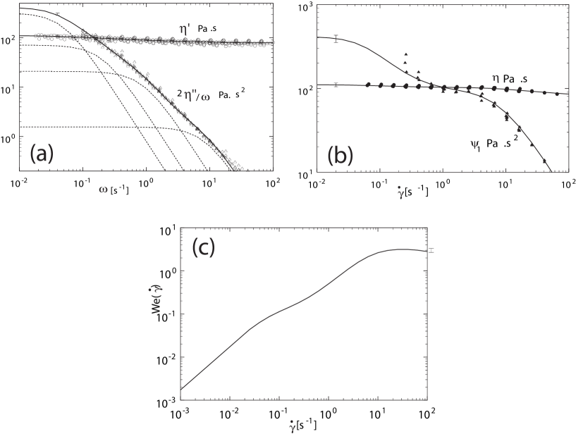
Figure 2: (a) Linear viscoelastic properties $\eta^{\prime}(\omega)$ and $2\eta^{\prime\prime}(\omega)/\omega$ of the $0.30$ wt % PIB in PB test fluid. The solid line is the fit of a four-mode Maxwell model to the data and the dashed lines are the individual spectral contributions, $(2\eta^{\prime\prime}/\omega)_{k}$. Error bars are given on the upper-left corner of the graph. (b) Steady shear material functions, $\eta(\dot{\gamma})$ and $\Psi_{1}(\dot{\gamma})$ of the test fluid. The solid lines are fits of the four mode Giesekus model to the data. Error bars are again shown in the upper left corner of the plots. (c) Plot of the shear rate dependent Weissenberg number, $We(\dot{\gamma})\equiv\lambda(\dot{\gamma})\langle\dot{\gamma}\rangle$ as a function of shear rate for the $0.30$ wt% PIB in PB test fluid. An error bar which applies to the part of the curve with shear rate larger than 0.25 s^-1 is also shown.

The dynamic shear flow material functions, $\eta^{\prime}(\omega)$ and, $2\eta^{\prime\prime}(\omega)/\omega$ of the 0.30 wt% polyisobutylene (PIB) in polybutene (PB) test fluid were measured in small-amplitude oscillatory shear flow in a cone-and-plate configuration and are shown in Figure 2(a). This linear viscoelastic data, in conjunction with the steady data shown in Figure 2(b), was used to fit a four-mode linear Maxwell model; the parameters of which define the relaxation spectrum which we have presented elsewhere [14]. Each mode is seen to be dominant in a different region of the spectrum; a given mode starts to shear-thin once a critical frequency $\omega_{k}\sim\lambda_{k}^{-1}$ is exceeded. In the case of, $\eta^{\prime}$ a similar pattern can be observed for the modal contributions, $\eta^{\prime}_{k}$, originating from the high molecular weight solute; however, these contributions are not shown since the contribution of the non-frequency-thinning solvent, $\eta^{\prime}_{s}=\eta_{s}$, dominates over the other modes.

Steady shear flow material functions were measured using the rheometer in the cone-and-plate and in the parallel-plate configurations. Plots of $\eta(\dot{\gamma})$ and $\Psi_{1}(\dot{\gamma})$ are shown in Figure 2(b). The linear Maxwell fit indicated a decrease in viscosity from $\eta_{0}$ = 110 Pa.s to 90 Pa.s at the maximum shear rate, for which data was obtained, of 40 s^-1. Because of this decrease of only 18% in the viscosity over nearly three decades of shear rate the test fluid closely approximated an elastic, constant viscosity non-shear-thinning Boger fluid. The highest shear rate for which material functions were measured was 40 s^-1; at shear rates exceeding this value viscous heating would act to decrease $\eta$ by more than 9% and $\Psi_{1}$ by more than 18%. Substantial shear thinning is observed for the first-normal-stress coefficient. The zero-shear-rate limit for $\Psi_{1}$ could not be reached because of the sensitivity limits of the normal force transducer. However, at 0.25 s^-1, the lowest shear rate for which results reproducible to within 25% could be obtained, the data indicated a lower bound on the zero-shear-rate limit of $\Psi_{1}>200$ Pa.s². The nonlinear viscoelastic four-mode Giesekus model is capable of capturing the shear thinning of the material functions; values of $\alpha_{k}$, which control the shear thinning behavior of the steady shear material functions, in addition to the coefficients $\eta_{k}$ and $\lambda_{k}$ are published elsewhere [14].

The stress-optical coefficients were determined using a Couette cell apparatus. For a given shear rate, the stress components in the fluid were determined from the previously measured viscometric functions. The birefringence and extinction angle of the fluid undergoing shearing were measured using the FIB system. The refractive index tensor n in the flow of a polymer blend is related to the component polymer contributions to the stress tensor as ${\bf n}=C_{\mathrm{PIB}}{\mbox{\boldmath$\tau$}}_{\mathrm{PIB}}+C_{\mathrm{PB}}\mbox{\boldmath$\tau$}_{\mathrm{PB}}$ where $C_{\mathrm{PIB}}$ is the stress-optical coefficient of the polyisobutylene solute, and $C_{\mathrm{PB}}$ is the corresponding coefficient for polybutene solvent. For all shear rates accessible with the rheometer used, the polybutene solvent exhibited Newtonian behavior. The difference in the normal components of the refractive index tensor arose exclusively from the contribution of the polyisobutylene solute component. From the experimental data it was estimated that $C_{\mathrm{PB}}=0.98\times 10^{-9}\pm 0.07\times 10^{-9}$ Pa^-1 and $C_{\mathrm{PIB}}=1.48\times 10^{-9}\pm 0.18\times 10^{-9}$ Pa^-1. The effect of form birefringence (see [14] for more details)on the measurement of $C_{\mathrm{PIB}}$ was minimal since the isotropic refractive index of the polybutene solvent matched that of the polyisobutylene solute, $n_{\mathrm{PB}}=n_{\mathrm{PIB}}=1.50$.

Use of the longest relaxation time, $\lambda_{1}$, is appropriate for flows with low characteristic shear rates, ${\dot{\gamma}}_{\mathrm{low}}$, such that for the shorter relaxation times associated with the other modes one obtains $\lambda_{k>1}\dot{\gamma}\ll 1$. However, because of the shear thinning nature of the fluid, use of the longest relaxation time will over-predict the characteristic relaxation time for elevated flow rates. We use the rate dependent Weissenberg number

$$We\equiv\lambda(\dot{\gamma})\langle\dot{\gamma}\rangle={\psi_{1}(\dot{\gamma})\over{2\eta(\dot{\gamma})}}\langle\dot{\gamma}\rangle.$$ (2)

to characterize the importance of elastic effects in our experiments. The effect of elasticity in the presence of shear thinning taken into consideration via the shear-rate dependent relaxation time $\lambda(\dot{\gamma})$. A plot of $We(\dot{\gamma})$ is shown in Figure 2(c). Predictions of $\Psi_{1}(\dot{\gamma})$ and $\eta(\dot{\gamma})$ were obtained from the fitted Giesekus model. Relaxation modes with time scales as great as 20 s were fit to the shear rheology information; reproducible dynamic data were obtained for frequencies as low as 0.1 s^-1. The plot shown is corroborated by experimental viscometric material function data for $\dot{\gamma}\geq 0.25$ s^-1. However, for smaller shear rates, the plot represents an extrapolated prediction of the fitted Giesekus model.

The highest value of mean upstream shear rate attained in the 2:1 contraction experiments is $\langle{\dot{\gamma}}_{\mathrm{Up}}\rangle=4.9$ s^-1, which corresponds to $We_{\mathrm{Up}}=1.80$; this value is within the range of the steady shear flow rheological data. The lowest value of up-stream shear rate for which an experimental result (taken in the 32:1 contraction) is reported is $\langle{\dot{\gamma}}\rangle_{\mathrm{Up}}=0.0021$ s^-1, which corresponds to $We_{\mathrm{Up}}=0.004$. The maximum value of the Reynolds number based on downstream conditions for a test run in this study is $7\times 10^{-4}$ so that inertial effects were negligible.

IV Spatiotemporal transitions in the structure of flow states

In general, a characteristic shear rate is selected so that global transitions in the flow field associated with elastic phenomena correspond with $We\sim O(1)$. However, in flow regions with shear rates above the selected characteristic value, local elastically induced flow phenomena may occur at Weissenberg number much less than one. Consequently, a Weissenberg number, $We_{\mathrm{Up}}$ , based on the upstream mean shear rate, $\langle{\dot{\gamma}}_{\mathrm{Up}}\rangle=\langle v_{z}\rangle/H$, is used to present our results. Several considerations motivate this choice. Firstly, $We_{\mathrm{Up}}$ can be determined solely from information on flow conditions for a given test run and known shear rheological data. Our experimental results indicate that onset of the instability is associated with flow conditions (shear rate and streamline curvature) upstream of the contraction plane. Furthermore, the critical $We_{\mathrm{Up}}$ for onset of instability onset is observed to decrease with increasing contraction ratio; in flows through geometries with large contraction ratios, $H/h\geq 8$ for instance, very low values of the critical $We_{\mathrm{Up}}$ viz, $We_{\mathrm{Up,crit}}\ll 1$ are observed. This suggests that the $We_{\mathrm{Up}}$ alone does not capture the physics controlling onset of instability. It is more intuitive to select the smallest length scale in the problem and consequently a Weissenberg number based on downstream conditions to characterize the flow patterns. In fact, we do interpret results in terms of both upstream and downstream definitions and find that either by itself is insufficient to characterize critical behavior. Consequently, we choose $We_{\mathrm{Up}}$ as the parameter of study.

We begin with an examination of the spatio-temporal structure of flow states and transitions observed. Off-centerline scans in space and time-series data acquired at a point are used to identify the $We_{\mathrm{Up}}$ at onset of instability as well as associated spatial wavenumbers and temporal frequencies.

IV.1 Velocity-field visualization

IV.1.1 Flow transitions in the 8:1 contraction

We first present data for the 8:1 contraction obtained from light sheet visualization of the flow at different flow rates.

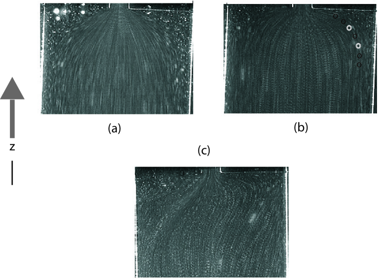
Figure 3: Side view of viscoelastic flow through the abrupt 8:1 planar contraction:(a) low flow rate with converging streamlines and Moffat vortex in outer corner, $We_{\mathrm{Up}}=0.052$ (number of superimposed frames ($N_{\mathrm{frames}}$) = 15, time interval between frames ($(\Delta t)_{\mathrm{frames}}$) = 0.33 s); (b) reduction in size of corner vortex and flattening of streamlines (shown by the sequence of circles following one streamline) indicating development of diverging streamlines , $We_{\mathrm{Up}}=0.108$ ($N_{\mathrm{frames}}$ = 10, $(\Delta t)_{\mathrm{frames}}$ = 0.20 s). The black circles interspersed by white circles are a guide to the eye indicating the onset of flattening.; (c) asymmetric, three-dimensional structure at high flow rates, $We_{\mathrm{Up}}=0.229$ ($N_{\mathrm{frames}}$ = 4, $(\Delta t)_{\mathrm{frames}}$ = 0.12 s). Arrow marks the direction of the flow.

Snapshots of the $yz$-plane streakline velocity patterns at various Weissenberg numbers are shown in Figure 3. For $We_{\mathrm{Up}}=0.052$ as shown in Figure 3(a), the flow field of the test fluid resembles the Newtonian flow profile. Specifically, the $yz$-plane streakline image indicates that the streamlines converge smoothly from the upstream channel into the downstream duct and that the flow is steady and symmetric about the center-plane $(\upsilon=0)$. The $xz$-plane images give no indication of flow in the $x$-direction. The resolution of the streakline images is insufficient to determine quantitatively the reattachment length of the outer vortex ($L_{v}$) in the upstream channel. However, the streakline image is consistent with an eddy in the outer corner with reattachment length of $L_{v}/H$ = 0.34. We note that this flow field has been predicted numerically and analytically for Stokes flow ($Re=0$) of a Newtonian fluid [15,16].

As $We_{\mathrm{Up}}$ is increased, the stream-lines still appear symmetric about the center-plane; however, instead of uniformly converging to the center-plane as the downstream slit is approached, the streamlines indicate divergence especially in a region approximately one half-height $H$ upstream of the contraction plane ($\zeta=0$). This onset firsts manifests as a tendency of the streamlines to flatten rather than curve continuously. The distance in the $z$-direction over which the streamlines exhibit the most rapid continuous convergence from the up-stream channel to the downstream slit moves closer to the contraction plane - cf. Figure 3(b)- than is seen for the lower $We_{\mathrm{Up}}$. An apparent decrease in the reattachment length of the outer corner vortex is associated with this streamline shift. More detailed observations suggest that this apparent streamline pattern is due to a transition to steady, three-dimensional flow for values of $We_{\mathrm{Up}}$ greater than approximately $0.124$.

Above $We_{\mathrm{Up}}=0.171$, the flow becomes fully time-dependent as well as three-dimensional. Although the flow is unsteady for $We_{\mathrm{Up}}>0.171$, snapshots at certain instants in time of the flow structure show features qualitatively similar to the patterns seen for $0.124<We_{\mathrm{Up}}<0.171$. Thus, qualitatively, one can learn about the structure of the three dimensional steady flow by looking at these snapshots. For instance, consider the streakline image of the flow in the $yz$-plane after onset of the spatial instability shown in Figure 3(c) for $We_{\mathrm{Up}}=0.229$. On the left half of the image the streaklines continuously converge from the upstream channel into the downstream slit. A separated vortex in the outer left corner is evident; the reattachment length of the vortex appears to be approximately $L_{v}/H\approx 0.3$, similar to that for the Moffat eddy for Newtonian flow. The in-plane flow speed $(v^{2}_{x}+v^{2}_{y})^{1/2}$ in the region immediately adjacent to the boundary of the left outer vortex is greater than in any other part of the image; a very high velocity gradient exists in the vicinity of the vortex boundary. In the upstream region of the flow ($\zeta<-0.2$), the $v_{z}$ velocity component of the flow is uniform throughout the left half of Figure 3(c), in contrast with the right side where the fast flow is located adjacent to the outer vortex. In the left half of the upstream region of the figure, streaklines initially approach the outer left wall; they move in the positive y-direction, away from the centerplane. When they near the outer left corner ($\zeta\geq-0.2$), the streaklines abruptly change direction and travel in the negative y-direction, following along the wall which defines the contraction plane ($\zeta=0$). No outer corner vortex could be observed on the right side of the image. When the streamlines reach the downstream slit, they change direction in order to enter the slit. Near the right entry corner of the downstream slit, a small but distinct vortex is observed. This lip vortex is separated from any vortical flow which may be present in the outer right corner. Although the most dramatic effect of the flow transition on the velocity field is observed near the outer walls and the contraction plane, the transition has a noticeable effect on the entire flow field up to at least a distance of approximately 1.5$H$ before the contraction plane. Specifically, the streaklines near the center-plane appear sinuous: the mean direction of flow is in the positive $z$-direction, and the streaklines have a sinusoidal shape in the $y$-direction.

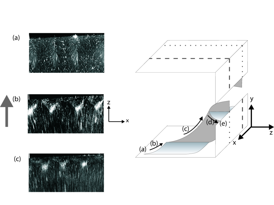
Figure 4: (A) Top view of the abrupt 8:1 planar contraction at high flow rate, $We_{\mathrm{Up}}$ = 0.229 ($N_{\mathrm{frames}}$ = 15, $(\Delta t)_{\mathrm{frames}}$ = 0.1 s for all images). Structure is three-dimensional, slices in the $xz$ plane at different $y$-elevations are shown: (a) flow near the outer wall ($\upsilon$ = -7.5), fluid flows in the $x$-direction to feed regions of fast flow visible as bright areas; (b) far from the contraction plane fluid feeds the fast regions, near the contraction plane fluid spreads out to assume a more uniform profile in the x-direction, $\upsilon$ = -4.0; (c) at $\upsilon$ = -2.0, closer to the centerplane, the flow is more uniform in the x-direction, within the triangular structures fluid wells up from planes closer to the outer wall. (B) Diagram representing the three-dimensional structure of the flow after onset of the instability: (a) far upstream fluid near wall fluid element travels in $z$-direction; (b) at distance order $H$ before contraction plane element feeds into fast region; (c) element in fast region flows toward downstream slit; (d) at distance order $h$ before contraction plane fluid spreads out to achieve $v_{z}$ more uniform along $x$; (e) fluid enters downstream slit.

Onset of temporal instability at high $We_{\mathrm{Up}}$

As $We_{\mathrm{Up}}$ is increased further beyond a value equal to 0.171, onset of temporal instability is observed at a critical flow rate. Thus the flow for $We_{\mathrm{Up}}=0.229$ is time dependent.

Frozen images (taken at a particular instant in time) of slices in the $xz$-plane located at positions ranging from near the outer wall to near the center-plane for a Weissenberg number of 0.229 are shown in Figure 4(A). These are discussed in order of increasing $\upsilon$ position, starting from near the outer wall and following the mean flow of fluid toward the downstream slit. At a position $\upsilon=-7.5$, streaks oriented in the $z$-direction are visible. These streaks have a mean separation from each other in the $x$-direction of about 1.5$H$; this separation defines the wavelength of the three-dimensional flow. The fluid in the vicinity of the streaks has a much faster $v_{z}$-component than fluid in the intermediate regions. Moreover, fluid is observed to flow out of the intermediate regions in the $x$-direction and feed into the streaks; this accounts for the arced appearance of the streaklines on either side of the fast streaks. In the slice at $\upsilon=-4.0$, the fast flow regions continue to be fed by the slow flow at distances greater than 0.3$H$ upstream of the contraction plane. Near the contraction plane the flow spreads out to assume a more uniform profile of $v_{z}$ along the x-direction. Specifically, fluid appears to travel along the bright boundaries which demarcate the triangular structures between the contraction plane and the end of a given streak. In the interior of these triangular structures, the flow is directed primarily in the $y$ (out-of-plane) direction. An image of a slice at $\upsilon=-2.0$ is shown in Figure 4(A-c). Here the triangular structures are confined to a region nearer to the contraction plane. Although the resolution of the streakline image is limited, careful study of the source videotape indicated that within the triangular structures there was flow in the $x$-direction, directed away from the center of the structure. The primary direction of flow within the triangular structures was still in the $y$-direction, toward the center-plane. Throughout the image (with the exception of the region located immediately before the contraction plane, where the triangular structures are located) the $v_{z}$ -component of the flow is more uniform along the $x$-direction than the slices taken closer to the outer wall (Figures 6(a) and 6(b)). Hence, close to the centerplane ($\upsilon=0$), the flow rearranges to adopt a more uniform velocity profile along the x-direction before entering the downstream slit.

It was observed that regions of fast flow on a given side of the center-plane correspond to regions of slow flow at the same $x$-position on the other half of the center-plane indicating the presence of bundles of counter-rotating vortex pairs having an interlaced structure. This was confirmed by continuously moving the $xz$ light sheet through the entire upstream height over a period of 45 s, much less than the time scale of the temporal oscillation.

From the light sheet slices in the $xz$- and $yz$-planes it is possible to reconstruct a qualitative sketch of the three-dimensional spatial structure of the flow valid as one extrapolates to the critical flow rate at which temporality onsets. The history of a fluid element traveling along a streamline which passes through the fast region of flow is illustrated schematically in Figure 4(B). Fluid near the wall of the upstream channel travels in the $z$-direction of mean flow (a). When it reaches a distance of the order of the upstream half-height, $H$, before the contraction plane, the fluid begins to also travel in the $x$-direction, toward the fast region (b). As it more closely approaches the fast region, the fluid begins to travel in the y-direction, away from the outer wall and towards the downstream slit (c). When the fluid approaches to within the order of the downstream slit half-height, $h$, of the contraction plane, it travels back in the positive $x$-direction, away from the center of the region of fast flow (d). The magnitudes of $v_{x}$ and $v_{y}$ are small when compared with that of $v_{z}$ when the fluid reaches the contraction plane (e). The spreading out of the flow near the contraction plane makes the $v_{z}$ component nearly uniform along the $x$-direction near the contraction plane $\zeta=0$.

The temporal structure of the instability is elucidated by sets of $yz$ and $xz$ sheet images taken successively in time. An image taken in the $yz$ plane of the flow through the 8:1 contraction is shown in Figure 5(a) and corresponds to $We_{\mathrm{Up}}=0.229$ at $t=0$ s; the streaklines are asymmetric with the region of fast flow on the right half of the image. An image in the $xz$ plane of the flow taken with the light sheet located near the outer wall, at $\upsilon=-7.8$, is shown in Figure 5(b). The $yz$ and $xz$ views were taken at different absolute times, but at the same flow conditions. Dashed arrows on a given image (e.g., $yz$ plane) indicate the position of the other image (e.g., $xz$ plane). At $t=105$ s, the streaklines (in Figure 5(c)) appear nearly symmetrical about the center-plane. The corresponding $xz$ image - Figure 5(d) - shows that the vortices have moved toward the center of the flow ( $\chi=0$). The flow field shown in Figure 5(e) at $t=270$ s is again asymmetric; however, the region of fast flow is now on the left half of the image. The flow in Figure 5(f) shows that the difference between Figures 5(e) and 5(a) is a result of the vortices having moved farther toward the center of the flow. Specifically, the region of fast flow in Figure 5(a) has been replaced by a region of slow flow in Figure 5(e).

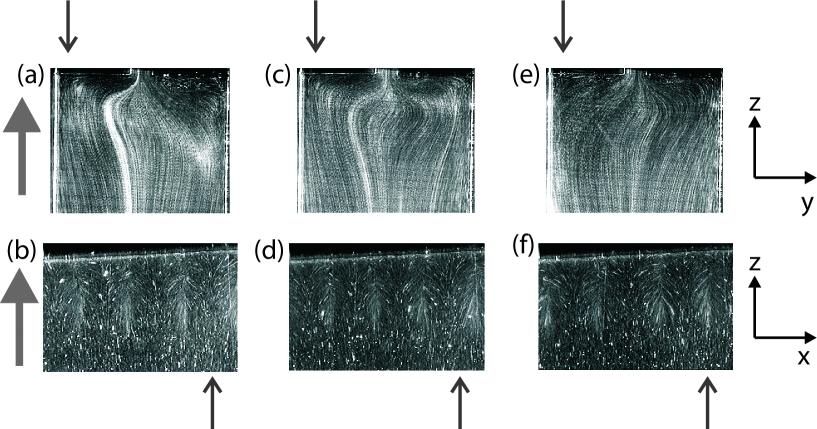
Figure 5: Successive images in time, $yz$- and $xz$-planes (fixed in space) of the abrupt 8:1 planar contraction at high flow rate, $We_{\mathrm{Up}}$ = 0.229 ($N_{\mathrm{frames}}$ = 15, $(\Delta t)_{\mathrm{frames}}$= 0.1 s for $yz$-images, $N_{\mathrm{frames}}$ = 40, $(\Delta t)_{\mathrm{frames}}$ = 0.1 s for $xz$-images): (a,b) views at t = 0 s, asymmetrical streaklines are shown in the $yz$-image with region of fast flow on the right half of the image; (c,d) views at t = 105 s, $xz$-image shows that vortex bundles have moved toward the center of the flow ($\chi$ = 0), streaklines in the $yz$-image appear nearly symmetrical; (e,f) views at t = 270 s, the $yz$-image shows asymmetrical streaklines, now with the fast flow on the left side of the image, $xz$-image shows that vortex bundles have moved toward the center of the flow, the fast flow region in (b) has been replaced by a slow flow region.

The flow closest to the walls bounding the $x$-directions ($\chi=\pm 32$) could not be observed with light sheet slices in the $y$ or the $xz$ plane; only positions in the range $-23\leq\chi\leq 23$ were accessible. However, visual observations in conjunction with the LDV measurements indicated that after onset of the temporal instability the vortices in the flow are continuously born at the walls bounding the x-direction ($\chi=\pm 32$) and move toward the center ($\chi=0$) of the flow. As a result, the mean spacing between the vortex bundles decreases. Eventually a vortex bundle must be destroyed to maintain an average spacing between the bundles on the order of the upstream half-height. This occurs through one of two mechanisms. Two neighboring streamline bundles near the center of the flow may move closer to each other until they eventually merge into one. Alternately, a vortex bundle near the center of the flow may decrease in size and intensity as neighboring streamline bundles on either side approach. Eventually the streamline bundle in the middle disappears entirely; this process of absorption by neighboring bundles, is shown in Figure 6 via successive $xz$-images in time. A destruction mechanism which has elements of both the merging and absorption processes, i.e. preferential absorption into one of the neighboring vortex bundles, was also observed.

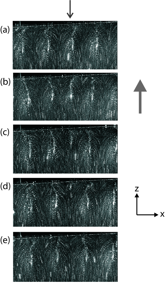
Figure 6: Successive streakline images in time, top view, of the abrupt 8:1 planar contraction at high flow rate, $We_{\mathrm{Up}}$ = 0.229 ($N_{\mathrm{frames}}$ = 6): (a) t = 0 s, vortex bundles of equal strength are evenly spaced $1.5H$ apart, note the arrow at top which indicates the location of the center vortex bundle on which attention is focused here; (b) view at t = 120 s, the vortex bundles have moved toward the center of the flow ($\chi$= 0), resulting in closer spacing; (c) at t = 180 s vortex bundles have moved yet closer together and the center vortex bundle has weakened relative to the neighboring bundles; (d) at t = 210 s the center vortex has weakened further and is barely distinguishable; (e) at t = 240 s the center bundle vortex has been completely absorbed into the neighboring bundles.

IV.1.2 Flow transitions in the 2:1 and 32:1 contractions

The flow transition sequence with increasing $We_{\mathrm{Up}}$ in the 2:1 contraction was qualitatively similar to that observed in the 8:1 contraction. However, the transitions occurred at higher values of $We_{\mathrm{Up}}$ . The wavelength and the upstream extent of the spatial instability were both of the order of the upstream half-height, $H$, as found for the 8:1 contraction. There were visual indications of time-dependent behavior of the vortex bundles at elevated flow rates. The movement of the vortices in the $xz$-plane was not as distinct as in the images acquired with the 8:1 contraction flow.

In the 32:1 contraction, the low aspect ratio, $W/2H=1$, of the upstream channel affected the transition sequence and spatio-temporal structure of the flow. Onset of three-dimensional flow, specifically flow in the $x$-direction, could be detected via light sheet visualization at the periphery of the observable region encompassing $-23\leq\chi\leq 23$. Additional detail on the spatio-temporal structure of the flow after onset of the instability is given in the sections to follow.

IV.2 Off-centerline velocity measurements of global flow transitions

Quantitative velocity field information was obtained to characterize the spatial and temporal structure of flows after, and the class of bifurcation at instability onset; the laser Doppler velocimetry (LDV) technique was used. To parallel the qualitative observations discussed above, results are given for transitions occurring at increasing $We_{\mathrm{Up}}$. Off-centerline LDV data were taken for the 2:1 and 32:1 contractions but not for the 8:1 contraction.

IV.2.1 Transition to and evolution of three-dimensional flow in the 2:1 contraction

The LDV system was operated with the frequency tracker in order to characterize the wavelength of the three-dimensional flow field in the $x$-direction after onset of the instability. Specifically, the measuring volume was scanned through the region corresponding to $-26<\chi<0$, $\upsilon=-1.75$, $\zeta=-1.80$ with the scan velocity $v_{x,{\mathrm{s}can}}$ held constant at 1.43 mm/s. The velocity data measured as a function of time were then converted to velocity as a function of spatial position. Data could not be obtained for $\chi>0$ because the backscattered light used in the LDV had to travel through too much fluid to yield a measurable signal.

As the volumetric flow rate was increased from an initially low value, the structure of the flow field evolved spatially through a sequence of transitions - first, onset of three-dimensional, steady flow, then wavenumber doubling and subsequent appearance of multiple harmonics.

Spatial profile of $v_{z}$ at intermediate $We_{\mathrm{Up}}$

At volumetric flow rates corresponding to $We_{\mathrm{Up}}\leq 0.37$, the profile of $v_{z}$ versus $x$ was uniform, and the flow was two-dimensional. When the flow rate was increased to values corresponding to $0.51\leq We_{\mathrm{Up}}\leq 1.37$, the profile of $v_{z}$ versus $x$ was no longer uniform, a transition to a three-dimensional, steady flow had occurred.

The frequencies of the flow-structure information (0.1 Hz and 1.5 Hz) and instrument induced noise (about 14 Hz) were well separated, and so a power spectrum (PS) of the data was used to identify oscillations associated with the temporal structure of the viscoelastic flow instability. The PS of the velocity versus position data was calculated by using data in the range $-26.1<\chi<-1.6$, for which the strongest signal was obtained. To obtain a more accurate estimate of the PS, a set of eight velocity versus position scans was made for a given flow rate. The Welch windowing function was applied to each scan before calculation of the PS. The eight power spectra were then averaged to generate a mean PS with a standard deviation corresponding to 35 % of a single PS.

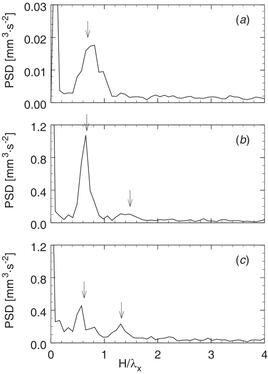
Figure 7: (a) Mean power spectrum (PS) of scan in the $x$-direction ($\upsilon$ = -1.75, $\zeta$ = -1.79) for flow through the 2:1 contraction with $We_{\mathrm{Up}}$ = 0.67. Mean dimensionless wavenumber of primary peak is $\overline{(H/\lambda_{x})_{1}}=0.69$; (b) PS of scan in $x$-direction ($\upsilon$ = -1.75, $\zeta$ = -1.79), 2:1 contraction, $We_{\mathrm{Up}}$ = 1.53. Wavenumber doubling behavior; primary peak wavenumber is $\overline{(H/\lambda_{x})_{1}}=0.67$, secondary peak wavenumber is $\overline{(H/\lambda_{x})_{1}}=1.48$; (c) PS of scan in $x$-direction ($\upsilon$ = -1.74, $\zeta$ = - 1.80), 2:1 contraction, $We_{\mathrm{Up}}$ = 1.72. Primary peak wavenumber is $\overline{(H/\lambda_{x})_{1}}=0.62$, secondary peak wavenumber is $\overline{(H/\lambda_{x})_{2}}=1.32$. Higher order harmonics (in addition to the primary and secondary peaks) are present. Note that the mean dimensionless wavenumber of the peaks shown in (a - c) are indicated by arrows.

A plot of the mean power spectral density (PSD) as a function of the dimensionless wavenumber, $H/\lambda_{x}$, where $\lambda_{x}$ is the wavelength in the $x$ direction is shown in Figure 7(a) for $We_{\mathrm{Up}}=0.67$. Wavenumber is used for the abscissa since the PS is calculated for equal wavenumber intervals. The large peak centered about $H/\lambda_{x}=0.69$ corresponds to the characteristic wavelength of the three-dimensional flow. The partial peak at the extreme left of the plot is an artifact and is not physically significant.

The power associated with the peak representing the spatial oscillation in the PS was estimated by summing the power spectral density (PSD) values of a continuous range of wavenumbers for which the PSDs were greater than ten percent of the peak value. The amplitude of a peak in the PS is defined as the square root of this total power under the peak; the spatial oscillation shown in Figure 7(a) has an amplitude of 0.065 mm s^-1. Since the peak has a finite breadth, an estimate of the wavenumber of the spatial oscillation should consider the entire peak, not only the wavenumber associated with the maximum power. Therefore, the wavenumbers were weighted with their associated PSD values and summation performed over the range. The sum was then normalized with the total power over the range to determine the first moment corresponding to the mean wavenumber. The characteristic dimensionless wavenumber of the spatial oscillation calculated in this fashion was $H/\lambda_{x}=0.74$, which corresponds to a wavelength of $\lambda_{x}=1.35H$.

Wavenumber doubling behaviour of spatial oscillation in $v_{z}$ at high $We_{\mathrm{Up}}$

For volumetric flow rates corresponding to $1.14\leq We_{\mathrm{Up}}\leq 1.53$, a secondary peak was observed at approximately twice the spatial wavenumber of the primary peak. The PS of the flow for $We_{\mathrm{Up}}=1.53$ is shown in Figure 7(b). The primary peak has $H/\lambda_{x}=0.67$; a broad secondary peak with a dimensionless wavenumber of 1.48 is also apparent.

Multiple harmonics in spatial oscillation in $v_{z}$ at high $We_{\mathrm{Up}}$

The PS of a flow with $We_{\mathrm{Up}}=1.72$ is shown in Figure 7(c). The secondary peak at $H/\lambda_{x}=1.32$ has increased in strength, whereas the primary peak at $H/\lambda_{x}=0.62$ has weakened. Additional peaks appear between the primary and secondary peaks and below the primary peak. The PSD values for these additional peaks are above the level of the broadband noise, indicating that these peaks represent additional harmonics. However, the resolution of the PS (the wavenumber interval) is limited by the finite distance in the $x$-direction which can be probed, and the limited number of data sets restricts the accuracy of the PSD estimate at a given wavenumber. These considerations prevent specific identification of the higher order harmonics.

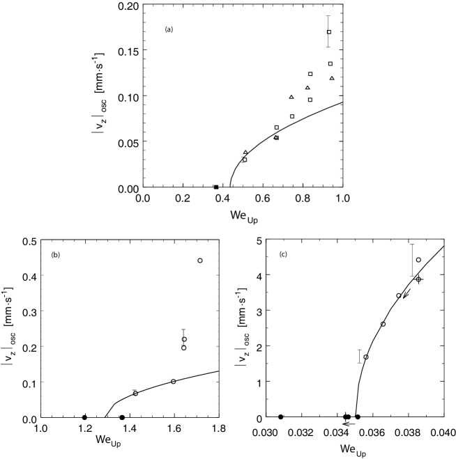
Figure 8: (a) Amplitude of spatial oscillation, $|v_{z}|_{osc}$, from scans of $v_{z}$ vs. $\chi$ ($\upsilon$ = -1.75, $\zeta$ = - 1.80) as a function of $We_{\mathrm{Up}}$ in 2:1 contraction flow . Data ($\Delta$) taken with successively increasing flow rates; ($\Box$) decreasing flow rates; note the absence of hysteresis. Solid symbols indicate two-dimensional flow; hollow symbols denote three-dimensional flow; (-), fit of equation to data near onset. The order 10 % error associated with the determination of the amplitude of oscillation is indicated by the two representative error bars. (b) Amplitude of oscillation, $|v_{z}|_{osc}$, for temporal instability at the point $\chi$ = -20.0, $\upsilon$ = -1.75, $\zeta$ = -1.80 as a function of $We_{\mathrm{Up}}$ in 2:1 contraction flow. Solid symbols indicate steady flow; hollow symbols denote time-dependent flow; (-), square-root-scaling fit to data near onset. The order 10% error associated with determination of the amplitude of oscillation is indicated by the two representative error bars; (c) Amplitude of oscillation, $|v_{z}|_{osc}$ , for time-dependent flow at the point $\chi$ =-21.0, $\upsilon$ =-1.50, $\zeta$ =-1.50 as a function of $We_{\mathrm{Up}}$ in the 32:1 contraction. Solid symbols indicate steady flow; hollow symbols denote time-dependent flow; (-), square-root-scaling fit to data near onset. Note that the fit slightly under-predicts the value of $We_{\mathrm{Up}}$ at onset of instability. (+) symbols and associated arrows indicate that in one of the runs the volumetric flow rate was decreased from $We_{\mathrm{Up}}$ = 0.0386 to $We_{\mathrm{Up}}$ = 0.0345; hysteresis was not observed. The order 10% error associated with determination of the amplitude of oscillation is indicated by the two representative error bars.

A transition to time-dependent behavior occurs in the range $1.37\leq We_{\mathrm{Up}}\leq 1.43$; the frequency associated with this temporal oscillation is of order 0.006 Hz. In contrast, the output from the tracker which contains the information on the spatial period of the instability for the scan speed used corresponds to a frequency between 0.1 and 1.5 Hz. Therefore, the time-dependent behavior does not have a deleterious effect on the measurement of the spatial form of the instability.

Classification of bifurcation to spatial oscillation

The amplitude of the spatial oscillation for flow through the 2:1 contraction is plotted as a function of $We_{\mathrm{Up}}$ in Figure 8(a). In order to check for the occurrence of hysteresis, the volumetric rate was first set to a value such that the flow was in the two-dimensional base state; specifically $We_{\mathrm{Up}}\leq 0.37$. Measurements of the velocity profile were then made at successively increasing flow rates; the amplitude of a peak associated with the spatial oscillation for a given $We_{\mathrm{Up}}$ is shown in the plot. In a second set of runs, the flow rate was initially set to a value such that the flow was in the three-dimensional and steady state. Velocity profile measurements were then taken at successively decreasing flow rates; the peak amplitudes for these measurements are also shown. Since there is no significant difference between the amplitudes of the sequences of measurements conducted for increasing and for decreasing flow rates, no hysteresis is evident. The standard deviation of the amplitude of oscillation of the eight power spectra which were averaged together was of order 10%; error bars of 10% are also indicated. The two-dimensional, steady base flow is indicated by a filled symbol and three-dimensional flow by hollow symbols.

Experimental observations indicate that in the absence of hystersis, the bifurcation is likely to be a supercritical pitchfork bifurcation. For this type of bifurcation, the amplitude of the spatial oscillation of the bifurcating parameter, $v_{z}$, close to onset, is expected from theoretical considerations [17-19], to scale with the control parameter, $We_{\mathrm{Up}}$ as

$$|v_{z}|_{\mathrm{osc}}=C_{\mathrm{S2}}(We_{\mathrm{Up}}-We_{\mathrm{Up,S2}})^{1/2},$$ (3)

where $C_{\mathrm{S2}}$ is a constant. The letter in the subscript of parameters in Equation (3) indicates the particular flow transition with which the parameter is associated: S indicates transition from two-dimensional, steady to three-dimensional, steady flow; T denotes transition from steady to time-dependent flow. The number indicates the contraction ratio, $H/h$, for which the parameter applies. A similar equation also arises in instabilities of Newtonian fluids at high Reynolds numbers [15,17]. Assuming that this expression indeed holds, we use equation (3) to fit our experimental data near the value of $We_{\mathrm{Up}}$ for onset. This procedure yielded $C_{\mathrm{S2}}=0.124$ mm s^-1 and the critical value $We_{\mathrm{Up,S2}}=0.44\pm 0.07$. The error bounds are derived from data points with $We_{\mathrm{Up}}$ immediately greater than or less than $We_{\mathrm{Up,S2}}$ for which stability of the base flow or spatial oscillation was observed. For $We_{\mathrm{Up}}>0.74$, a departure from the square root scaling is clearly observed. We posit that this behavior is associated with the onset of harmonics of the fundamental wavenumber of the spatial oscillation.

IV.2.2 Transition to Time-dependent flow in 2:1 contraction

In order to study the temporal structure of the flow after transition to time-dependent behavior, the measurement volume of the LDV system was placed at the point $\chi$ =-20.0, $\upsilon=-1.75$, and $\zeta$ =-1.80. This point was chosen since it was expected to provide the clearest signal; specifically, in the spatial scan it was within the region of maximum difference between the crest and trough of the measured $v_{z}$. The flow rate was then set to a value corresponding to a specific $We_{\mathrm{Up}}$, and the velocity recorded as a function of time. The evolution in the temporal structure of the flow is described here; the classification of the bifurcation to time-dependent behavior is given at the end of this section.

At volumetric flow rates corresponding to $We_{\mathrm{Up}}\leq 1.37$, no characteristic temporal oscillations were observed in the power spectrum. Increasing the volumetric flow rate to a value corresponding to $We_{\mathrm{Up}}\geq 1.43$ revealed oscillations in the time-series data, which were characterized by calculating the power spectrum in a similar manner as for the space data. Overlapping data sets were extracted from the time series; the Welch windowing function was applied to each set; individual PS were calculated; and the results were averaged to compute a mean PS with a lower standard deviation than the individual PS. The PS of at least three time-series segments were averaged together, with each segment consisting of approximately 900 data points representing 1500 s of flow. The mean frequency was calculated in a manner analogous to the calculation of the mean wavelength for the spatial instability. As an example, for $We_{\mathrm{Up}}=1.72$, the primary peak had a mean frequency of 0.0047 s^-1, which corresponded to a period of 214 s.

Our experimental results indicate that the spatial oscillation of the three-dimensional flow undergoes wavenumber doubling. For $We_{\mathrm{Up}}\geq 1.80$ the power of the secondary peak in the temporal PS exceeded that contained in the primary peak; an increase in the amplitude of the secondary peak with $We_{\mathrm{Up}}$ and a decrease for the primary peak also was noted in the PS of the spatial oscillation discussed above.

We expect that the onset of periodic motion from the steady state is via a super-critical Hopf bifurcation. Such a bifurcation could either be subcritical (exhibiting hysteresis) or supercritical (without hysteresis) [17].

For a super-critical Hopf-bifurcation, square-root scaling of the amplitude near onset of temporal oscillation is expected and we check our data to see if this is the case. Let us first consider Figure 8(b) wherein the amplitude of the temporal oscillation is plotted as a function of $We_{\mathrm{Up}}$. Steady flow is indicated by the solid symbols; time-dependent flow, by the hollow symbols. Noise in the data made it difficult to characterize the amplitude of oscillation near the onset of the time periodic instability. For the data points with representing oscillation of finite amplitude, the error was of order 10%, as shown in the graph. A square root scaling of the form in Equation (3) but now recognized as applying to temporal bifurcations was applied to interpret the data. Unfortunately the measurement errors inherent in the data do not allow us to either support or disprove the scaling. One expects a square root scaling that is to be expected for a supercritical Hopf bifurcation, but the data by itself supports a 1/3 power. It is possible however that measurement errors and uncertainties might have resulted in this result being a fit rather than the square root. Further measurements are needed in the vicinity of the critical point. The fitted scaling parameters for the temporal instability in the 2:1 contraction were $C_{\mathrm{T2}}=0.183$ mm s^-1 with $We_{\mathrm{Up,T2}}=1.29$. Thus the square-root fit predicts a lower critical point for the onset of instability than is observed.

IV.2.3 Global flow transitions in the 32:1 contraction

LDV measurements were restricted by the size of the side window of the geometry to the region $-8\leq\upsilon\leq 8$. Velocity measurements near the wall of the upstream channel in the 32:1 contraction (at $\upsilon=\pm 32$) could not be obtained; hence, in order to measure a large amplitude of oscillation associated with a flow transition, the $v_{y}$-component of the flow was measured. Spatial scans in the x-direction as well as time series information at a given point were acquired with the LDV system operated in frequency tracker mode. Flow phenomena which span the entire $x$-dimension are considered here; phenomena localized near the wall at $\chi$ = $\pm$ 32 are considered later. We discuss the spatial structure of the instability in the 32:1 contraction first; then, the temporal structure is addressed.

Spatial structure of flow after onset of instability

In contrast to flow in the 8:1 and 2:1 contractions, a transition from the two-dimensional base flow to a three-dimensional, but steady, spatial structure that encompassed the entire span of the $x$-dimension was not observed. Rather, an immediate transition from the base flow to a three-dimensional, time-dependent flow spanning the $x$-dimension was observed.

LDV measurements were performed by moving the measuring volume in the negative $x$-direction at a constant rate of $v_{x,scan}=1.43$ mm s^-1. This scanning procedure did not lead to errors in measuring length scales, since the voltage output of the tracker during the spatial scans had a lowest characteristic frequency on the order of 0.05 s^-1 compared to the characteristic frequency of the temporal oscillation of 0.003 s^-1. Scans performed at different times for $-32\leq\chi\leq 0$, $\upsilon=-1.50$, and $\zeta=-1.50$ for a flow with $We_{\mathrm{Up}}=0.039$ indicated the formation of a wave originating at the bounding wall at $\chi=-32$ and moving in the positive $x$-direction towards the center of the flow. The results suggested that a temporal oscillation was superimposed upon a steady, spatial oscillation. The amplitude of the temporal oscillation seemed to be greatest near the wall; this prevented accurate characterization of the wavelength, amplitude, or onset $We_{\mathrm{Up}}$ of an underlying steady, spatial oscillation. The amplitude of the temporal oscillation was observed to decrease as the center of the flow was approached and the pattern of the underlying spatial oscillation became distinct.

Characterization of onset and temporal structure of flow transition

To characterize the temporal structure of the instability in the 32:1 contraction, the measurement volume was placed at the point $(\chi,\upsilon,\zeta)=(-1.50,-21.0,-1.50)$, the flow rate was set to a value corresponding to a specific $We_{\mathrm{Up}}$, and the velocity recorded as a function of time. The evolution of the temporal structure of the flow for successively greater Weissenberg numbers was followed. Characterization of the dependence of the magnitude of the oscillation on the Weissenberg number was used to identify the critical value for onset of the instability.

For $We_{\mathrm{Up}}\leq 0.0352$ no time dependence of $v_{y}$ was detected in the region scanned. When the volumetric rate was increased to $We_{\mathrm{Up}}\geq 0.0356$, oscillations were apparent in the time-series data. The PS was calculated and the mean frequency of the oscillation peak was found to be 0.0029 s^-1. The amplitude of oscillation is plotted as a function of $We_{\mathrm{Up}}$ in Figure 8(c). For $We_{\mathrm{Up}}>0.0356$, the amplitude was observed to increase monotonically until $We_{\mathrm{Up}}=0.0424$; beyond this point the onset of additional harmonics resulted in a decrease in the amplitude of the primary peak. No hysteresis was noted when $We_{\mathrm{Up}}$ changed from $We_{\mathrm{Up}}=0.0386$ to $We_{\mathrm{Up}}=0.0345$, which was just below the critical point.

The amplitude as a function of $We_{\mathrm{Up}}$ near the critical value was interpreted using

$$|v_{z}|_{\mathrm{osc}}=C_{\mathrm{T32}}(We_{\mathrm{Up}}-We_{\mathrm{Up,T32}})^{1/2},$$ (4)

with $C_{\mathrm{T32}}=68.2$ mm s^-1 and $We_{\mathrm{Up,T32}}=0.0350$ being the best-fit parameters. For $We_{\mathrm{Up}}=0.0352$ the flow is steady; hence, equation (4) slightly under predicts the critical $We_{\mathrm{Up}}$ for onset of instability. This discrepancy is most likely to be a consequence of error in the measurement. Notice however that unlike in the Figure 8(b), the agreement between the square-root scaling anticipated and that observed is very good indicating that the bifurcation corresponds to a supercritical Hopf bifurcation. Thus in summary, the temporal oscillations, the lack of hysteretic behavior and the expectation of a supercritical Hopf bifurcation motivate the square root scaling of amplitude at onset.

For high volumetric rates corresponding to $We_{\mathrm{Up}}\geq 0.0424$, pronounced secondary harmonic peaks are visible in the PS. The characteristic frequencies of the secondary peaks adjacent to the primary peak were consistent with doubled and halved harmonics of the fundamental frequency. However, the signal-to-noise ratio of the velocity data was too low to allow more detailed classification of the time-periodic flow in the nonlinear regime.

IV.3 Local evolution of flow near the bounding wall at $\chi=\pm 32$ in the 32:1 contraction

We also observed a viscoelastic flow transition localized near the wall bounding the $x$-dimension for flow through the 32:1 contraction. The spatial structure of this transition was characterized by making LDV measurements with the frequency tracker. The measuring volume was scanned in the x-direction at a constant rate of $v_{x,scan}=1.43$ mm/s through the region of space corresponding to $-32\leq\chi\leq 0$, $\zeta=-1.50$ for $\upsilon$ = -1.50 and +1.50. The acquired set of velocity versus time data was then converted to velocity versus spatial position data. Confidence in the profile was improved by reproducing the measurements; a set of eight scans was used to develop a given profile.

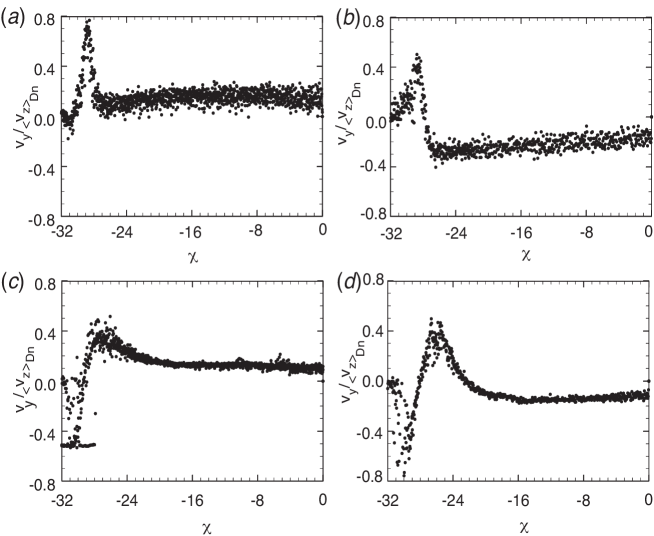
Figure 9: Dimensionless $v_{y}$ vs $\chi$ plots for flow through the 32:1 contraction (a) $We_{\mathrm{Up}}=0.006$, $\upsilon=-1.50$, (b) $We_{\mathrm{Up}}=0.006$, $\upsilon=+1.50$, (c) $We_{\mathrm{Up}}=0.031$, $\upsilon=-1.50$, and (d) $We_{\mathrm{Up}}=0.031$, $\upsilon=+1.50$.

The profiles for $We_{\mathrm{Up}}=0.006$ are shown in Figures 9(a) and 9(b). In the middle section, $-24\leq\chi\leq 0$, the flow appears uniform to within the accuracy of the measurement. The velocity is positive for $\upsilon=-1.50$ and the fluid flows up toward the center-plane; for $\upsilon=+1.50$, the velocity is negative. The signal-to-noise ratio is low in these measurements because of the slow flow rate. Near the wall, $-32\leq\chi\leq-24$ the flow is nonuniform in the $x$-direction. In particular, the flows in the middle section ($-24\leq\chi\leq 0$) on either side of the center-plane are in opposite directions; however, the peak of the spike, located at $\chi=-29$, is positive for both $\upsilon=-1.50$ and $\upsilon=+1.50$. The spike is neither a measurement artifact nor a transient resulting from finite response time of the tracker electronics.

The velocity profile is illustrated in Figures 9(c) and 9(d) along the $x$-direction for $We_{\mathrm{Up}}=0.031$. The flow is still steady; the onset of time-dependent behavior occurred at $We_{\mathrm{Up,T32}}=0.036$. The velocity profile near the center of the flow ($-20\leq\chi\leq 0$) is uniform and in opposite directions for $\upsilon=-1.50$ and $\upsilon=+1.50$. The nonuniform region of the profile has expanded to fill the range $-32\leq\chi\leq-20$ and both positive and negative values of $v_{y}$ are seen. Specifically, for the range $-32\leq\chi<-28$ the velocity is negative on both sides of the center-plane, while for $-28<\chi\leq-24$ the velocity is positive on both sides.

The velocity profiles observed are consistent with the flow near the $\chi$ = -32 wall having a vortex structure in the $xy$-plane. At the lower flow rate, $We_{\mathrm{Up}}=0.006$, the elliptic point of the vortex is located close to the wall, in the range $-32\leq\chi\leq-30.5$. At higher flow rates, the vortex increases in size, with the elliptic point located within the region $-29.5\leq\chi\leq-28$. This vortex growth is a non-Newtonian phenomenon. At the low flow rate, $We_{\mathrm{Up}}=0.006$, the phenomenon is probably purely local, in extent as well as origin; the extent of the vortex is on the order of the downstream length scale, $h$, not the upstream length scale, $H=32h$.

In the vicinity of the downstream slit, the fluid near the wall experiences a higher shear rate than fluid at other locations in the $x$-direction with the same $y$ and $z$ values because of the additional no-slip boundary. This higher shear rate results in onset of an instability which is localized near the wall. At higher flow rates, we expect the global flow to interact with the local instability. When wall effects are negligible and two-dimensional flow is closely approximated throughout the geometry, the length scale of the spatial instability is set by the upstream half-height, $H$. However, for the 32:1 contraction ratio, the width of the geometry is only $W=2H$. Therefore, the increased extent of the vortex at $We_{\mathrm{Up}}=0.031$, may result from expansion of the local vortex near the wall, or could be a manifestation of the global spatial instability observed for the 2:1 and 8:1 contractions additionally modified by the presence of the bounding walls located at $x=\pm 32h=\pm H$.

In flows through the 2:1 and 8:1 contraction geometries, the upstream aspect ratios are sufficiently high ($W/2H=$ 16 and 4, respectively), that the presence of a bounding wall at the extremes of the $x$-direction can be treated as a local imperfection to the two-dimensional base flow and to flow transitions at elevated Weissenberg number. For the 32:1 contraction the upstream aspect ratio is unity; consequently, the walls bounding the $x$-direction affect the flow structure and the transition sequence throughout the upstream channel. In the 2:1 and 8:1 contractions, the local instability near the bounding walls at $\chi=32$ noted in the 32:1 contraction is also anticipated to occur. The global time-dependent flow may be influenced by the local flow transition which acts as a perturbation that sets the direction of movement of the vortices, from the bounding walls toward the center of the flow, $\chi=0$.

IV.4 Quantitative characterization of centerline velocity profile evolution

The flow transition to three-dimensional, steady flow described earlier appears to be associated with changes in the centerline profile. This phenomenon was studied in detail by operating the LDV system using burst analysis to measure the centerline velocity profile at several flow rates for the 2:1, 8:1, and 32:1 contractions. Upstream of the contraction plane, a decrease in the centerline velocity below the value for the fully developed upstream channel flow was noted at elevated $We_{\mathrm{Up}}$. Close to the contraction plane, in the entry flow region, an increase in the local elongational strain rate was observed.

IV.4.1 Centerline velocity profile evolution in the 2:1 contraction

The magnitude of the $v_{z}$ velocity component along the centerline in the middle of the flow was measured for the 2:1 contraction; specifically, scans were performed over the range $(\chi=0,\upsilon=0)$, and $-40\leq\zeta\leq 12$. The velocity data as a function of position, $v_{z}(z)$ was fit to a cubic spline. From this, the strain-rate profile as a function of position, $\dot{\epsilon}=\partial{v_{z}}/\partial{z}$ was obtained. The maximum dimensionless strain rate, $\dot{\epsilon}_{\mathrm{max}}(h/{\langle v_{z}\rangle}_{\mathrm{Dn}})$, was used to quantify the sharpness of the peak in the centerline strain-rate profile.

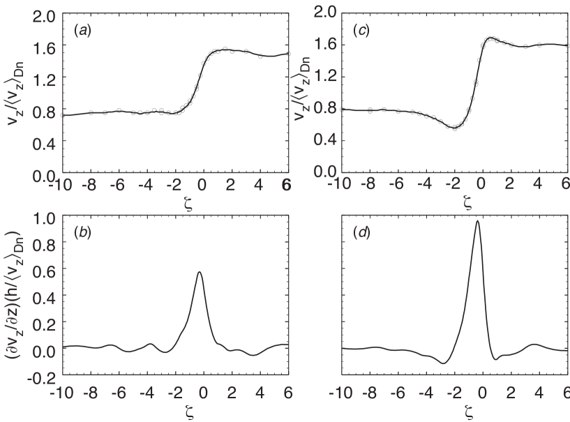
Figure 10: Centerline ($\upsilon$ = 0) velocity and elongational strain-rate profiles for 2:1 contraction flow: (a) Dimensionless $v_{z}$ vs. $\zeta$, $We_{\mathrm{Up}}$ = 0.37; (b) Dimensionless $\dot{\epsilon}$ vs. $\zeta$, $We_{\mathrm{Up}}$ = 0.37; (c) Dimensionless $v_{z}$ vs. $\zeta$, $We_{\mathrm{Up}}$ = 1.20; (d) Dimensionless $\dot{\epsilon}$ vs. $\zeta$, $We_{\mathrm{Up}}$ = 1.20. $(o)$ velocity data; (-) cubic spline fit.

Results for $We_{\mathrm{Up}}=0.37$ are shown in Figure 10(a). Far upstream of the contraction plane ($\zeta<-8$), the profile in the $y$-direction is parabolic. The centerline velocity made dimensionless with the downstream mean velocity is approximately $v_{z}/{\langle v_{z}\rangle}_{\mathrm{Dn}}\approx{3\over 2}h/H$. When a fluid element approaches to within two down-stream half-heights of the contraction plane ($\zeta>-2$) it suddenly accelerates to the downstream fully developed centerline velocity, $v_{z}\approx{3\over 2}{\langle v_{z}\rangle}_{\mathrm{Dn}}$. The dimensionless strain rate $(\partial{v_{z}}/\partial{z})(h/\langle v_{z}\rangle_{\mathrm{Dn}})$ is shown in Figure 10(b) as a function of axial position. The acceleration of the fluid occurs over the range $-2\leq\zeta\leq 1.5$. The maximum dimensionless strain rate of 0.57 is observed at a position $\zeta=-0.31$, immediately up-stream of the contraction plane. At a higher flow rate corresponding to $We_{\mathrm{Up}}=1.20$, diverging flow is evident along the centerline. As shown in Figure 10(c), the fluid initially decelerates from the fully developed upstream velocity and then accelerates near the contraction plane. Another contrast with the centerline velocity profile for low $We_{\mathrm{Up}}$ is that a pronounced velocity overshoot is observed immediately downstream of the contraction plane. The centerline strain-rate profile for $We_{\mathrm{Up}}=1.20$ is shown in Figure 10(d). Diverging flow is evident as a region of negative strain rate for $-6\leq\zeta\leq-2$; the minimum centerline velocity occurs at $\zeta=-2.1$, and the velocity overshoot appears as a region of negative strain rate located downstream of the con-traction plane which extends over the range $0.5\leq\zeta\leq 3$.

The maximum dimensionless strain rate achieved for high $We_{\mathrm{Up}}$ flow is substantially greater than for low $We_{\mathrm{Up}}$. This effect is attributable to two factors. Firstly, the difference between the minimum upstream and maximum downstream dimensionless velocity is greater for the higher value of $We_{\mathrm{Up}}$ because of the diverging flow and velocity overshoot. Secondly, the region where the fluid accelerates from the upstream into the downstream slit decreases slightly in extent, from $-2\leq\zeta\leq 1.5$ for $We_{\mathrm{Up}}=0.37$ to $-2\leq\zeta\leq 0.5$ for $We_{\mathrm{Up}}=1.20$. Note that this flow rearrangement is related to the elastic nature of the flow since the Reynolds number is low.

IV.4.2 Centerline Velocity Profile Evolution in 8:1 and 32:1 contractions

The profiles of the centerline velocity and the corresponding centerline strain-rate were also studied for flow through the 8:1 and 32:1 contractions. At $We_{\mathrm{Up}}=0.070$, the strain-rate profile for the 8:1 contraction appears qualitatively similar to that for the 2:1 contraction; however, in the 8:1 contraction the axial region over which the flow accelerates from the upstream into the down-stream slit is larger. Additionally, in contrast with the 2:1 contraction flow, the strain-rate profile is composed of two distinct regions, a high strain rate region and a low strain rate upstream tail. These two regions become more pronounced as the contraction ratio is increased to 32:1. The precise distance that this tail extended upstream could not be determined for the 32:1 con-traction due to restrictions in the LDV measurements. For example, in the 32:1 contraction at a Weissenberg number of 0.038, the region of greatest strain rate is restricted to $-2\leq\zeta\leq 0.25$. As the Weissenberg number increases, the distinction between the high strain-rate region and low strain-rate tail becomes clearer.

IV.4.3 Evolution of Centerline Velocity Profile

The centerline profiles for the flows through the different contraction ratios exhibit similar qualitative features. At low $We_{\mathrm{Up}}$ , there are two distinct regions of positive strain rate through which a fluid element on the centerline passes when accelerating from the slit upstream of the contraction plane to the slit downstream of the contraction plane. A low strain-rate upstream tail is evident in the profiles for the 32:1 and 8:1 contractions. The upstream extent of the tail appears to be set by the upstream half-height, $\zeta\sim H/h$ (although the restriction on LDV measurement to $\zeta\geq-40$ did not allow identification of the precise extent in the 32:1 contraction). At the location $\zeta\approx-3$, upstream of the contraction plane, the tail region adjoins a high strain-rate peak. The location of the transition between the low strain-rate tail and high strain-rate peak appears to be set by the downstream half-height, $h$.

The existence of two distinct regions, one a long, low strain-rate upstream tail, the other a high strain-rate peak can be explained as follows. On the centerline and near the contraction plane, the flow field is governed primarily by the downstream slit; the region of high strain rate, the extent of which is set by the downstream half-height, is characteristic of this entry flow field. Stated another way, the flow near the slit does not see the upstream boundary conditions. Following this reasoning, a limiting profile is expected near the contraction plane for the case of an infinite contraction ratio (sink flow). However, for a flow with a finite contraction ratio, the upstream half-height, $H$, must play some role in determining the strain-rate profile. Specifically, the net Hencky strain experienced by a fluid element traveling along the centerline from the up-stream to the downstream regions is set by the ratio of centerline velocities of the upstream and downstream fully developed flows or

$$\epsilon_{\mathrm{Hencky}}=\ln{({{v_{z}(\upsilon=0)_{\mathrm{Dn}}}\over v_{z}(\upsilon=0)_{\mathrm{Up}}})}.$$ (5)

At a sufficient distance upstream of the contraction plane, the upstream boundary conditions set the profile for the low strain-rate up-stream tail, the spatial extent of which scales with the upstream half-height, $H$. A distinct transition between the upstream tail and downstream peak is not noted for the case of the 2:1 contraction, probably because the upstream and downstream half-heights are sufficiently similar that the two regions overlap.

A common set of flow phenomena also is noted for the flows through the different contractions at elevated $We_{\mathrm{Up}}$. Specifically, in contrast with the flows for low $We_{\mathrm{Up}}$, there is an increase in the maximum strain rate attained and a velocity overshoot is observed immediately downstream of the contraction plane. The spatial extent of the velocity overshoot in the downstream region is governed by the downstream half-height, $h$. This scaling is probably a result of the strain rate in the vicinity of the downstream slit being much higher than that in the low strain-rate upstream tail; the fluid only remembers flow conditions near the downstream slit.

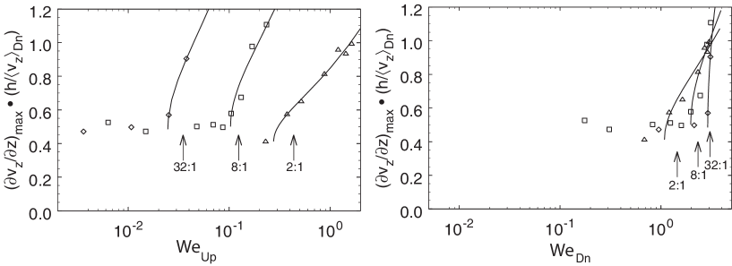
Figure 11: Maximum centerline dimensionless strain rate vs. Weissenberg number: ($\Delta$) 2:1 contraction; ($\Box$) 8:1 contraction; ($\lozenge$) 32:1 contraction. The lines are square-root fits to the data, the lower terminus of the line is the predicted onset point for the increase in dimensionless strain rate with Weissenberg number; the arrows indicate the value for which transition from global, two-dimensional base flow to three-dimensional flow occurs. (a) domain is Weissenberg number defined in terms of upstream flow parameters, $We_{\mathrm{Up}}$; (b) domain is Weissenberg number defined in terms of downstream flow parameters, $We_{\mathrm{Dn}}$.

At elevated flow rates, diverging flow was noted upstream of the contraction plane for the 2:1 and 8:1 contractions. The point of minimum centerline velocity occurred for the 2:1 and 8:1 contractions at the boundary between the diverging ($\partial{v_{z}}/\partial{z}<0$) and accelerating ($\partial{v_{z}}/\partial{z}>0$) flow regimes. The location of this minimum velocity point appeared to scale with the upstream half-height, $H$, moving further upstream with increasing $H$. Specifically, for the 2:1 contraction, the minimum was at $\zeta$ = -2.1; for the 8:1 contraction, at $\zeta$ = -5.5. No diverging flow was seen for the 32:1 contraction flow; however, since the farthest point upstream which could be probed was located at $\zeta$ = -40, this observation is consistent with a scaling with the upstream half-height, $H=32h$. For the case of the 8:1 contraction, after onset of diverging flow, the long upstream tail of low, positive strain rate did not extend as far upstream, reaching only to $\zeta$ = -5.5 instead of $\zeta\sim-10$; a limited number of data points prevents precise delineation of this change in extent.

The transition from a moderately peaked to a sharply peaked strain-rate profile occurs smoothly over an intermediate range of $We_{\mathrm{Up}}$. The maximum dimensionless strain rate is shown as a function of $We_{\mathrm{Up}}$ in Figure 11(a) for the three contraction ratios investigated. A square-root function of the form

$${\dot{\epsilon}}_{\mathrm{max}}(We_{\mathrm{Up}})({h\over{{\langle v_{z}\rangle}_{\mathrm{Dn}}}})-{\dot{\epsilon}}^{0}_{\mathrm{max}}({h\over{{\langle v_{z}\rangle}_{\mathrm{Dn}}}})=C(We_{\mathrm{Up}}-We_{\mathrm{Up,crit}})^{1/2}$$ (6)

was fit to each data set associated with a given contraction ratio. In equation (6), $We_{\mathrm{Up}}$ is the independent variable, and ${\dot{\epsilon}}^{0}_{\mathrm{max}}({h\over{{\langle v_{z}\rangle}_{\mathrm{Dn}}}})$ is the maximum dimensionless centerline strain rate in the limit of zero Weissenberg number, as inferred from the data which is also used to fit the constants $C$ and $We_{\mathrm{Up,crit}}$. Our experimental observations are consistent with a supercritical bifurcation; however, there are not sufficient data points for the bifurcation to be definitively classified. Thus, these square-root fits are intended to act primarily as a guide to the eye.

Two regions are apparent for the data associated with a given contraction ratio. At low $We_{\mathrm{Up}}$, the maximum dimensionless strain rate is nearly independent of $We_{\mathrm{Up}}$; this independence is evident for $We_{\mathrm{Up}}<0.1$ for 8:1 contraction flow and for $We_{\mathrm{Up}}<0.02$ for 32:1 contraction flow. At larger $We_{\mathrm{Up}}$ the maximum dimensionless strain rate increased with $We_{\mathrm{Up}}$. Upstream diverging flow and downstream velocity overshoot are noted in the velocity profile for elevated volumetric flow rates; these phenomena result in the increase in maximum dimensionless strain rate. Since the Weissenberg number is defined in terms of the upstream flow parameters, the critical value for transitions can be substantially less than unity. This reflects the dependence of the flow rearrangement on contraction ratio as well as on $We_{\mathrm{Up}}$.

The maximum dimensionless strain rate as a function of the Weissenberg number defined in terms of the mean downstream shear rate; i.e. $We_{\mathrm{Dn}}=We({\langle v_{z}\rangle}_{\mathrm{Dn}}/h)$ is shown in Figure 11(b). The critical parameters for the onset of diverging flow differ by only a factor of 3 between $H/h=2$ and $H/h=32$, as opposed to the corresponding parameters from Figure 11(a), which differ by a factor of 20. However, distinct superposition of the curves is not observed. This is attributed to the role which the contraction ratio plays in governing the flow rearrangement. It is clear that neither the upstream nor downstream based Weissenberg number alone fully describes the conditions for transition to diverging flow.

To decide whether the upstream or downstream definition is the more appropriate one to use, it is helpful to consider the critical Weissenberg number for flow rearrangement expected in the limits of $H/h\rightarrow 1$ (channel flow) and $H/h\rightarrow\infty$ (sink flow). For the sink-flow limit, it is expected that $We_{\mathrm{Dn,crit}}$ is a non-zero, finite value. Specifically as $H/h\rightarrow\infty$ , the upstream walls have less and less effect on what occurs in the vicinity of the downstream slit. In contrast, $We_{\mathrm{Up,crit}}$ will continuously decrease and approach zero. In the channel-flow limit, it necessarily follows that $\lim_{H/h\rightarrow 1}$ $We_{\mathrm{Up,crit}}$=$We_{\mathrm{Dn,crit}}$. In a channel, rearrangement to diverging flow is never observed; two scenarios may be envisioned as occurring as the lower limit is approached. 1) The critical Weissenberg number may continuously approach infinity as the contraction ratio approaches one. In this case $We_{\mathrm{Up,crit}}$ will monotonically increase with $H/h$, whereas $We_{\mathrm{Dn,crit}}$ will first decrease and then increase. 2) The critical Weissenberg number will approach a finite limit as $H/h\rightarrow 1$ . $We_{\mathrm{Up,crit}}$ will continuously increase, and $We_{\mathrm{Dn,crit}}$ continuously decrease to the limit as channel flow is approached. By consideration of the critical values shown in figures 11(a) and 11(b), this limiting value (should Scenario 2 apply) can be bounded as $\lim_{H/h\rightarrow 1}$ $0.3<We_{\mathrm{Dn,crit}}$=$We_{\mathrm{Up,crit}}<1.1$. Note, however, that when the limit $H/h=1$ is reached, the solution will vanish since diverging flow does not occur in channel flow. Hence, as the contraction ratio increase from the channel- to the sink-flow limit, $We_{\mathrm{Up,crit}}$ will monotonically decrease, regardless of whether Scenario 1 or Scenario 2 applies. This decrease reflects the importance of both nonlinear elastic effects (as parameterized by $We_{\mathrm{Up,crit}}$) and the imposed boundary conditions (as parameterized by $H/h$) in determining rearrangement to diverging flow; i.e. diverging flow is not noted in a channel of $H/h=1$. In contrast, $We_{\mathrm{Dn,crit}}$ increases with contraction ratio, at least over a certain range of $H/h$. Furthermore, $We_{\mathrm{Dn,crit}}$ will not necessarily exhibit a monotonic dependence on $H/h$. These considerations motivate and support the use of the Weissenberg number defined in terms of upstream flow conditions throughout this paper.

V Interpretation of results using transition maps

In the previous sections, qualitative flow visualization studies and quantitative LDV measurements used to characterize the evolution of the flow field with increasing $We_{\mathrm{Up,crit}}$ for a set of planar contraction geometries were described. These results are used now to develop a unified picture of velocity field transitions in viscoelastic planar contraction flow. Characteristic length and time scales of flow structures after the transitions are identified and related to dimensions of the geometry. The viscoelastic scaling described in the introduction is used to understand the onset of instability in planar contraction flow in terms of the interaction of elastic stresses oriented in the streamwise direction with streamline curvature. Finally, a correlation between the onset of diverging flow and global, spatial flow transition is noted.

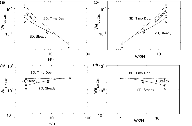
Figure 12: Maps of transitions observed in viscoelastic planar contraction flow: (a) critical $We_{\mathrm{Up}}$ vs. contraction ratio, $H/h$; (b) critical $We_{\mathrm{Up}}$ vs. upstream aspect ratio, $W/2H$. Experimentally observed transitions are denoted: ($\blacklozenge$), onset of increase in maximum dimensionless centerline strain rate with $We_{\mathrm{Up}}$; ($\times$) diverging flow; ($\blacksquare$) , transition from tow-dimensional, steady base flow to three-dimensional, steady flow; ($\square$), transition from steady to time-dependent flow; ($\bullet$), secondary spatial harmonics; ($\bigcirc$) secondary spatio-temporal harmonics. Fits are denoted: (solid line) , transition from two-dimensional, steady base flow to three-dimensional, steady flow; (dashed line), transition from steady to time-dependent flow; (c) critical $We_{\mathrm{Dn}}$ vs. contraction ratio, $H/h$; (d) critical $We_{\mathrm{Dn}}$ vs. upstream aspect ratio, $W/2H$. Experimentally observed transitions are denoted: ($\blacklozenge$), onset of increase in maximum dimensionless centerline strain rate with $We_{\mathrm{Dn}}$; ($\times$) diverging flow; ($\blacksquare$), transition from two-dimensional, steady base flow to three-dimensional, steady flow; ($\square$), transition from steady to time-dependent flow; ($\bullet$), secondary spatial harmonics; ($\bigcirc$) secondary spatio-temporal harmonics. Fits are denoted: (solid line) , transition from two-dimensional, steady base flow to three-dimensional, steady flow; (dashed line), transition from steady to time-dependent flow.

V.1 Flow transition maps

The series of ordered flow transitions denoted by the critical value of $We_{\mathrm{Up}}$ are shown in Figures 12(a) and 12(b) as a function of the contraction ratio, $H/h$ and the upstream aspect ratio. It is clear from Figure 12(a) that the 2:1 and 8:1 contractions exhibit a common transition sequence: two-dimensional rearrangement to diverging flow, transition from two-dimensional to three-dimensional and steady flow, and onset of time-dependent flow.

V.1.1 Transitions in the 2:1 and 8:1 Contractions

For $H/h=2$ and 8 the flow is two-dimensional and steady at low values of $We_{\mathrm{Up}}$. As $We_{\mathrm{Up}}$ is increased above a lower critical value, the centerline velocity profile changes. The flow begins to diverge upstream of the contraction plane, and velocity overshoot is observed downstream of the contraction plane; both phenomena are associated with an increase in the maximum dimensionless centerline strain rate. As the flow rate is increased above the lower critical value, a subsequent supercritical bifurcation to three-dimensional and steady flow throughout the upstream region was observed. For the 2:1 contraction, wavenumber doubling behavior was detected at yet higher values of $We_{\mathrm{Up}}$.

The next transition observed with increasing volumetric flow rate was a bifurcation to time-dependent flow, corresponding to a supercritical Hopf bifurcation. As discussed earlier the amplitude of the temporal oscillation of $v_{z}$ grew continuously and monotonically with $We_{\mathrm{Up}}$, consistent with the scaling of a supercritical Hopf bifurcation. The flow pattern close to criticality has temporal oscillations (traveling waves) superposed on the spatial oscillation (stationary waves). To understand this flow structure, consider the appearance of the time series if there were no superposition and the waves associated with the spatial oscillation suddenly started to move as a unit from the bounding wall toward the center of the flow. A sudden jump, not a gradual increase, in the amplitude of temporal oscillation would be observed at a given point in space. Videotaped streakline images in the $xz$-plane of the 2:1 contraction were studied; there were indications that the spatio-temporal structure after onset of the temporal instability was more complex than that of a single set of waves traveling at a uniform velocity in the $x$-direction. However, the precise spatio-temporal structure could not be determined from these streakline images.

The flow visualization observations of the temporal instability for the 8:1 contraction indicated that the vortex bundles traveled from the walls of the geometry toward the center of the flow; no underlying stationary wave pattern was observed. However, streakline visualization may not detect low amplitude oscillations near onset. Only images of the central region of the flow could be acquired. Since the amplitude of the temporal oscillation was greatest near the bounding walls, the flow visualization technique may not have been capable of resolving superposed temporal and spatial waves near onset of the temporal instability. The observation via light sheet visualization in the 8:1 contraction of moving streamline bundles without an underlying stationary pattern, is probably a result of the $We_{\mathrm{Up}}$ being substantially greater than the critical value for onset of temporal instability, so that large amplitude traveling waves dominated over low amplitude stationary waves.

V.1.2 Flow transitions in the 32:1 contraction

For flow through the 32:1 contraction, we found that at low values of $We_{\mathrm{Up}}$, the flow was steady and two-dimensional. As $We_{\mathrm{Up}}$ was increased above a critical value, an increase in the maximum dimensionless centerline strain-rate was observed. However, diverging flow was not seen; the strain rate was positive at all points on the centerline upstream of the contraction plane.

At still higher values of $We_{\mathrm{Up}}$, a direct transition from globally steady, two-dimensional flow to a three-dimensional, time-dependent flow was found. Two scenarios could explain this observation. One, the width of the geometry may have been too narrow for the steady, three-dimensional flow, characterized by spatial oscillation of $v_{z}$ in the $x$-direction, to occur. Alternately, it also is possible that onset of the temporal flow transition is the result of an interaction between the local flow transition noticed at the bounding wall and the global flow field. For high upstream aspect ratios, the local vortex at the wall would have to grow substantially, requiring higher values of $We_{\mathrm{Up}}$, before interacting with the entire flow field. In contrast, for low upstream aspect ratio, only a small amount of growth of this bounding wall vortex would be required, resulting in low values of $We_{\mathrm{Up}}$ for onset of the temporal instability. Hence, for the 32:1 contraction the extreme case of unit aspect ratio induces onset of the temporal oscillations before onset of steady, spatial oscillations. The latter view is supported by LDV measurements which indicated that the amplitude of the temporal oscillation was greatest near the bounding wall at $\chi=-32$ and weakest near the center of the flow $\chi=0$. At high flow rates, the onset of harmonics in the frequency spectrum was noted. These harmonics seemed to occur by the spatial wavenumber doubling of the wave structure and not doubling of the rate of wave propagation in the $x$-direction.

V.1.3 Summary of the transition maps

The maps illustrate that there are commonalities in the sequence of transitions which occur for increasing $We_{\mathrm{Up}}$ for different contraction ratios; however, the critical values of $We_{\mathrm{Up}}$ for these transitions decrease with increasing contraction ratio. The ratio of critical onset values, $We_{\mathrm{Up,T}}/We_{\mathrm{Up,S}}$ decreases between the contraction ratios 2:1 and 8:1 and apparently decreases to a value less than unity for the 32:1 contraction.

The critical value for onset of the spatial instability, $We_{\mathrm{Up,S}}$, appears to be directly related to the ratio of upstream to downstream half-height, $H/h$. We address this issue later. The onset of the temporal flow transition also appears to be closely related to the upstream aspect ratio, $W/2H$.

V.1.4 Transition maps in terms of downstream Weissenberg numbers

The transition map plotted in Figures 12(c) and 12(d) shows the critical Weissenberg number defined in terms of downstream flow parameters, $We_{\mathrm{Dn,crit}}$, as a function of contraction ratio or aspect ratio. This quantity defined in terms of the mean downstream shear rate for the spatial transition, $We_{\mathrm{Dn,S}}$, increases by a factor of two as $H/h$ increases from 2 to 8. This behavior may be contrasted with the four-fold decrease of $We_{\mathrm{Up,S}}$ for the same increase in $H/h$. Thus, when the range is defined in terms of $We_{\mathrm{Dn,S}}$, the curve associated with the spatial transition appears flatter than when the upstream Weissenberg number is used. Note, however, that whereas $We_{\mathrm{Up,S}}$ decreases with contraction ratio, $We_{\mathrm{Dn,S}}$ increases with contraction ratio. In subsequent sections, the relation of the critical Weissenberg number for the spatial transition to the streamline curvature around the outer corner which is induced by the greater-than-unity contraction ratio, $H/h>1$, is discussed. Consideration of the streamline-curvature interaction leads to the prediction that for increased curvature the critical Weissenberg number will decrease. The observation that the Weissenberg number decreases when defined in terms of upstream parameters but not when defined in terms of downstream parameters supports the use of the upstream Weissenberg number.

The critical value for transition from steady to time-dependent flow, $We_{\mathrm{Dn,T}}$, appears insensitive to contraction ratio. In contrast, the value of $We_{\mathrm{Up,T}}$ for the temporal transition exhibits a strong dependence on $H/h$. Superficially, this observation appears to indicate that the transition to time-dependent behavior is controlled by the parameter $We_{\mathrm{Dn}}$. However, in fact, the temporal transition appears to be related to flow conditions induced by the presence of a wall bounding the lateral sides of the upstream channel. In this scenario, an appropriate Weissenberg number could be defined in terms of the characteristic shear rate in the region near the centerplane, immediately adjacent to the wall bounding the x-dimension, and close to the contraction plane. Note that the width of the channel, $W$, and the half-height of the downstream channel, $h$, were fixed for all the experiments. Hence the characteristic shear rate alluded to is approximately proportional to the mean downstream shear rate. The flatness of the curve describing the temporal transition does not necessarily imply that downstream flow conditions control the spatial transition. Rather, this flatness may be related to a critical value of the characteristic shear rate and the particular geometry used for these experiments, in which the ratio of width to downstream half-height was constant at $W/2h=32$.

V.2 Characteristic length and time scales of flow structures

Characteristic length scales associated with the flow rearrangement to diverging flow and the spatial transition to three-dimensional flow were estimated from the measurements. These length scales were in turn related to geometric parameters of the planar contraction. A characteristic time scale was extracted for the temporal oscillation; however, this time scale could not be related to specific parameters of the flow or fluid rheology (e.g. the parameters characterizing the relaxation spectrum, $\lambda_{k}$). In addition, a length scale associated with the diverging flow was obtained by determining the distance of the point of minimum velocity on the centerline from the contraction plane at $\zeta=0$.

The wavenumber of the spatial oscillation after flow transition, made dimensionless with the upstream half-height, is plotted in Figure 13(a) as a function of $We_{\mathrm{Up}}$ for the 2:1 and 8:1 contraction ratios. For the 8:1 contraction, the dimensionless wavenumber increased with $We_{\mathrm{Up}}$; for the 2:1 contraction, no significant dependence of wavenumber on $We_{\mathrm{Up}}$ was noted. Above a critical value of $We_{\mathrm{Up}}$, but before onset of time-dependent flow, doubling of the spatial wavenumber in the 2:1 contraction was observed. Period doubling in the 8:1 contraction was not observed. The dimensionless wavenumber of the primary peak is of the same order for both the 2:1 and 8:1 contraction ratios, $H/\lambda_{x}\approx 0.7$. A three-dimensional and steady flow state was not seen in flow through a 32:1 contraction.

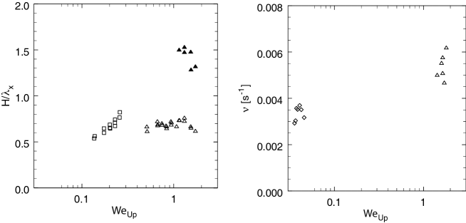
Figure 13: (a) Dimensionless wavenumber, $H/\lambda_{x}$, vs. $We_{\mathrm{Up}}$ after onset of three-dimensional flow: ($\square$) primary peak for the 8:1 contraction, streakline visualization data used; primary ($\bigtriangleup$) and secondary ($\blacktriangle$) peaks for the 2:1 contraction, LDV data used, scans performed over range $-26\leq\chi\leq-1.5$, $\upsilon$ = -1.75, $\zeta$ = -1.80. (b) Frequency ($\nu$ ) vs. $We_{\mathrm{Up}}$ after onset of time-dependent flow: ($\triangle$), 2:1 contraction, $v_{z}$ vs. $t$ series acquired at $\chi$ = -20.0, $\upsilon$ = -1.75, $\zeta$ = -1.80; ($\lozenge$) , 32:1 contraction, $v_{y}$ vs. $t$ series acquired at $\chi$ = -21.0, $\upsilon$ = -1.51, $\zeta$ = -1.51.

The characteristic frequency of the temporal oscillation is shown in Figure 13(b) as a function of $We_{\mathrm{Up}}$ for the 2:1 and 32:1 contraction ratios. The time-series data used to determine this frequency was acquired with the LDV measuring volume placed approximately half-way between the center of the flow and the bounding wall of the channel: at $\chi=-20$ for the 2:1 contraction, and at $\chi=-21$ for the 32:1 contraction. The results indicate only a weak dependence of frequency on contraction ratio: the frequency of oscillation in the 2:1 contraction is higher than the frequency in the 32:1 contraction. Note that the period associated with the oscillation was $T_{p}=180$ s for the 2:1 contraction and $T_{p}=340$ s for the 32:1 contraction. In both cases, the period is much greater than the estimated zero-shear-rate relaxation time of the test fluid, $\lambda_{10}=\psi_{10}/2\eta_{o}\sim 1$ s. No trend of the frequency was observed with variation of $We_{\mathrm{Up}}$, for a given contraction ratio. LDV measurements were not taken for the 8:1 contraction; data was obtained via analysis of videotaped streakline images.

V.3 Critical Weissenberg numbers and mechanism driving transitions

Consideration of structural features of the flow transitions and the scaling of onset $We_{\mathrm{Up}}$ with contraction ratio has elucidated the mechanism of viscoelastic instability in the planar contraction. In particular, these features were consistent with the interaction of streamwise elastic stress with streamline curvature around the outer corners of the planar contraction acting to induce flow transitions.

Shear flow rheological characterization of the Boger test fluid indicated that the fluid had a high zero-shear-rate relaxation time of $\lambda_{10}>1$ s. Inertia was negligible, $Re_{\mathrm{Dn}}=7\times 10^{-4}$, for all the flows investigated, whereas elastic memory or nonlinear effects could influence the flows, since $We_{\mathrm{Up}}$ as great as 1.8 were attained. Therefore, although some structural features of the flow after onset of instability resemble those of Görtler vortices, the transitions were induced by the elastic, not inertial, character of the flows. The characteristic length scales of flow structures indicate that the transitions were driven by interaction of elastic stresses in the streamwise direction with streamline curvature in the upstream region of the flow. Specifically, the extent of the oscillations associated with the flow transitions upstream of the contraction plane, as indicated by the reattachment length of the outer corner vortex adjacent to the fast flow region, was of the order of the upstream half-height, $H$. The wavelength of the spatial oscillation was quantitatively characterized via LDV scans in the neutral $x$-direction and found to scale with upstream half-height. The characteristic dimensions of the oscillation in the $x$- and in the $z$-directions indicate the relation of the flow transition to streamline curvature in the flow around the outer corner, rather than around the reentrant corner.

The spatial structure of the flow after onset of the instability bears resemblance to viscometric flows for which it has been concluded that interaction of streamwise normal stresses with curved streamlines drives the instability. To unify previous experimental observations of flow transitions, McKinley and co-workers [10] introduced and used the idea of transition maps. Employing physical arguments and scalings based on the linearized form of the governing equations, a dimensionless parameter was formulated that related a characteristic shear rate, streamwise stress, fluid residence time, and streamline curvature in a flow to a viscoelastic Görtler number, $M_{VG}$, given by

$$M_{VG}\equiv({{V\lambda_{p1}\over R_{c}}}{{\tau_{p11}\over{\eta\dot{\gamma}}}})^{1/2}.$$ (7)

This dimensionless quantity was found to set the conditions for the onset of instability for several viscometric and complex flows. The first term within the parentheses represents a ratio of a characteristic length over which perturbations to the viscoelastic stress relax to a characteristic radius of curvature in the flow, $R_{c}$. The relaxation length in the numerator is the product of a characteristic velocity $V$ and the characteristic relaxation time of the polymer, $\lambda_{p1}\equiv\psi_{1}/2(\eta-\eta_{s})$ where $\psi_{1}$ is the first normal stress coefficient, $\eta$ is the solution viscosity, and $\eta_{s}$ denotes the solvent viscosity. The second term within the parentheses represents the relative magnitude of the coupling of perturbative elastic stresses to the stresses in the base flow. The polymeric contribution to the streamwise stress is given by $\tau_{p11}$, and $\dot{\gamma}$ is a characteristic shear rate. For complex flows, parameters that relate the characteristic streamline curvature to geometric parameters must be computed or measured.

To understand the critical Weissenberg numbers observed in our experiments in more detail, we start with the relationship embodied in equation (7). The upstream half-height, $H$, is the characteristic length scale for the extent of the spatial oscillation upstream of the contraction plane and the wavelength of the oscillation; therefore, the flow transition seems to be related to streamline curvature around the outer corner of the contraction. Hence, it is natural to use the upstream flow conditions in obtaining characteristic values.

The characteristic curvature, $R_{c}^{-1}$, must approach zero as the contraction ratio approaches unity; this limit is equivalent to fully developed Poiseuille flow in a channel for which elastically-driven instabilities are not observed. As $H/h$ increases, the dimensionless curvature, $H/R_{c}$, of the streamlines around the outer corner of the contraction is expected to increase. A simple expression that captures this behavior is

$${H\over R_{c}}={1\over A}({H\over h}-1)^{B}$$ (8)

where the constants $A$ and $B$ are both positive. The velocity, $U$, and shear rate, $\dot{\gamma}$, are related to upstream flow conditions as

$$\dot{\gamma}={\langle\dot{\gamma}\rangle}_{\mathrm{Up}}=U/H=Q(2H^{2}W)^{-1},$$

where $W$ is the extent in the $x$-direction of the geometry and $Q$, the volumetric flow rate. This shear rate is used in the evaluation of the polymeric relaxation time, $\lambda_{p1}$, and the streamwise polymeric stress, $\tau_{p11}$. The expression for the critical condition for onset of flow instability in the planar contraction is re-written in terms of a critical upstream shear-rate-dependent Weissenberg number as

$$We_{\mathrm{Up,crit}}=M_{VG}({A(1-\eta_{s}/\eta)\over 2})^{1/2}({H\over h}-1)^{-B/2}=S({H\over h}-1)^{-B/2}$$ (9)

where the unknowns $A$ and $M_{VG}$ have been combined into a single term, $S=M_{VG}({A(1-\eta_{s}/\eta)/2})^{1/2}$. Experimental data for the critical upstream Weissenberg number, $We_{\mathrm{Up,S}}$, associated with the spatial flow transition in the 2:1 and 8:1 contractions are used to fit the unknown parameters. Specifically, a good match with the data for spatial transition was obtained with $S_{S}=0.44$ and $B_{S}/2=0.64$.

The conditions governing transition to time-dependent flow are more complex than those controlling onset of three-dimensional, steady flow. As mentioned earlier, a local flow transition near the wall bounding the $x$-dimension seems to play a role in the onset of the temporal transition; the vortex structure associated with this local transition scales with the downstream half-height, $h$, rather than the upstream half-height, $H$. The upstream aspect ratio, $W/2H$, in addition to the contraction ratio, $H/h$, together determine the $We_{\mathrm{Up,T}}$ for transition to time-dependent flow. Nevertheless, we obtain a reasonably good fit to the data for the critical $We_{\mathrm{Up}}$ for transition to time-dependent flow in the geometries with contraction ratio $H/h$ = 2, 8, and 32. The fitted parameters had values of $S_{T}=1.4$ and $B_{T}/2=1.1$; the root mean square of the fractional error of the fit was 3%. These fits have been plotted along with experimental data in the figures illustrating the flow transition.

The conditions governing transition to time-dependent flow may be more complex than those controlling onset of three-dimensional, steady flow. As discussed earlier, a local flow transition near the wall bounding the $x$-dimension seems to play a role in the onset of the temporal transition; the vortex structure associated with this local transition scales with the downstream half-height, $h$, rather than the upstream half-height, H. The upstream aspect ratio, $W/2H$, in addition to the contraction ratio, $H/h$, may determine the $We_{\mathrm{Up,T}}$ for transition to time-dependent flow. Nevertheless, equations (8) and (9) provide a good fit to the data for the critical $We_{\mathrm{Up}}$ for transition to time-dependent flow in the geometries with contraction ratio $H/h$ = 2, 8, and 32. The fitted parameters had values of $S_{\mathrm{T}}=1.4$ and $B_{\mathrm{T}}/2$ = 1.1; the root mean square of the fractional error of the fit was 3%.

When results for the critical Weissenberg numbers for the transition data are extrapolated to higher contraction ratios, the neutral stability curves for the predicted spatial (two-dimensional to three-dimensional flow) and temporal (steady to time-dependent flow) transitions intersect at a contraction ratio of approximately $(H/h)_{S}=15$. In the experiments, the contraction ratio was adjusted by varying the upstream channel half-height for a fixed downstream half-height. Hence, an increase in the contraction ratio results in a decrease in the upstream aspect ratio. Our results suggest that the point of intersection of the neutral stability curves corresponds to an upstream aspect ratio of $(W/2H)_{S}=2.1$. The dimensionless wavenumber for the 2:1 and 8:1 contractions was determined to be approximately $H/\lambda_{x}=0.7$. This provides an estimate of the number of wave cycles that would fit into the half-width of a geometry with an upstream aspect ratio of two: $W(2\lambda_{x})^{-1}=1.5\sim 1$. It is interesting that approximately one wave cycle of the spatial oscillation would fit into the half-width of the geometry with a contraction ratio such that $We_{\mathrm{Up}}$ is identical for onset of the spatial and temporal instabilities. This strongly supports the idea that transition to time-dependent flow is related to a three-dimensional imperfection introduced by the wall bounding the lateral dimension of the geometry. In particular, the base flow may make a direct transition to time-dependent flow in the 32:1 contraction since a full cycle of the spatial oscillation cannot fit into the half-width of the upstream channel.

As discussed earlier, for the 2:1 and 8:1 contractions, onset of three-dimensional, steady flow occurs for a $We_{\mathrm{Up}}$ immediately greater than the $We_{\mathrm{Up}}$ for which an increase in the maximum dimensionless centerline strain rate with $We_{\mathrm{Up}}$ is noted. A global transition to three-dimensional flow, distinct from the transition to time-dependent flow, was not noted for the case of the 32:1 contraction. However, the critical $We_{\mathrm{Up}}$ for direct transition from two-dimensional, steady to three-dimensional, time-dependent flow in the 32:1 contraction is greater than the critical $We_{\mathrm{Up}}$ for onset of increasing centerline maximum dimensionless strain rate with $We_{\mathrm{Up}}$. Hence, the relation between flow transition and the dependence of peak strain rate on $We_{\mathrm{Up}}$ for the case of the 32:1 contraction is consistent with the relation observed for the 2:1 and 8:1 contractions.

It is possible that the two-dimensional flow rearrangement associated with the diverging flow promotes onset of the three-dimensional and steady instability. In particular, visualization of flow in the $yz$-plane indicates that after onset of diverging flow, the streamlines near the outer corner become more tightly curved. A smaller characteristic radius of curvature of the streamlines in conjunction with an increase in the local strain rate, associated with shift of the streamlines toward the contraction plane, may allow the critical viscoelastic Görtler number, for onset of the instability, to be exceeded for a lower volumetric flow rate than if this two-dimensional streamline rearrangement did not first occur. This could explain why the critical Weissenberg number for transition to three-dimensional flow is immediately greater than the critical $We_{\mathrm{Up}}$ for onset of diverging flow.

VI Future perspectives and concluding remarks

Our experiments support the concept that the interaction of stream-wise stress with streamline curvature induces transition to three-dimensional flow in complex flows, such as in the planar contraction. Two interesting questions are yet to be understood satisfactorily. First, more detailed information on the stress-curvature mechanism which drives the transition to three-dimensional flow is required. Secondly, the influence of three-dimensionality in the base flow, introduced by the wall bounding the neutral $x$-dimension, on the flow transition sequence is yet to be understood. These walls are seen to act as an imperfection to the nominally two-dimensional base flow and alter the essential nature of the flow transition sequence.

There is evidence that a bifurcation of codimension-2 [18,19] exists at the point where the neutral stability curves for the spatial and the temporal transitions intersect on the transition map; this point occurs at approximately $H/h=15$ (or $W/2H=2.1$) and $We_{\mathrm{Up}}=0.08$. To achieve such a bifurcation two control parameters, in this case $H/h$ (or $W/2H$) and $We_{\mathrm{Up}}$, must be tuned to specific values. The transition from the two-dimensional, steady base flow in the planar contraction appears to be driven by the inter-action of stream-wise stress with streamline curvature. This implies that such a transition would be observed in an ideal, two-dimensional planar contraction flow. An imperfection in the form of finite, but large, upstream aspect ratio might modify this transition but would not be expected to change its basic structure.

The upstream aspect ratio, $W/2H$, is observed to play an essential role in defining the critical conditions for transition from steady to time-dependent flow but not for the spatial transition. This suggests that the transition map for viscoelastic flow through a planar contraction of finite upstream aspect ratio is most appropriately represented in a three-parameter space. The upstream Weissenberg number, the upstream aspect ratio $(W/2H)$, and the contraction ratio $(H/h)$ are the independent parameters that determine the flow state of the system and are each associated with a coordinate axis of the space. Figure 14 shows a qualitative transition map in this three-parameter space for flow through the planar contraction. The neutral stability boundary for the spatial transition from two-dimensional, steady base flow to three-dimensional, steady flow is represented as a two-dimensional surface within this space. In Figure 14, it is assumed that this spatial transition surface is nearly independent of aspect ratio. The neutral stability boundary identified with the steady to time-dependent temporal transition is represented as a second surface. This temporal transition surface is also assumed to be independent of contraction ratio to leading order. The intersection of the two neutral-stability surfaces defines a one-dimensional curve on which a codimension-2 bifurcation occurs.

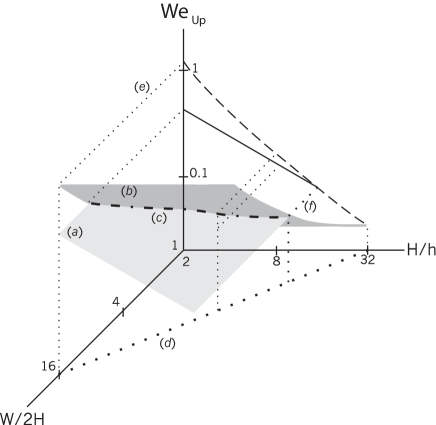
Figure 14: Hypothetical representation of flow transition map for the planar contraction in three-parameter space: ((a), light gray plane) neutral-stability surface for spatial transition from two- to three-dimensional steady flow; ((b), dark gray plane) neutral-stability surface for temporal transition from steady to time-dependent flow; ((c), $-.-$) curve for codimension-2 bifurcation at the intersection of the neutral stability surfaces; ((d), $---$) projection of the experimental subspace onto the ($W/2H,H/h$) plane; construction lines indicating the projection onto the ($We_{\mathrm{Up}},H/h$) plane of the intersection of the experimental subspace with neutral stability surfaces ((e), $....$) and with the curve representing the codimension-2 bifurcation ((f),$----$ ).

In the experiments presented here, the upstream aspect ratio, $W/2H$, and the contraction ratio, $H/h$, were simultaneously varied. The relation between the two parameters viz., the upstream and downstream aspect ratios are related to the contraction ratio simply by $W/2H=(W/2h)/(H/h)$. The downstream aspect ratio was constant throughout the experiments (with value $W/2h=32$). These relationships enable us to define a two-dimensional experimental subspace, which can be represented as a surface (invariant along the $We_{\mathrm{Up}}$ axis) in the three-dimensional transition map. The intersection of the experimental subspace with the given neutral-stability boundary is the one-dimensional subset of the boundary was probed in our experiments. Projection of the one-dimensional neutral-stability subsets onto the $(We_{\mathrm{Up}},H/h)$ and $(We_{\mathrm{Up}},W/2H)$ planes yields the two-dimensional transition map.

The concept of a three-parameter transition map discussed above is consistent with the experimental results but admittedly speculative. Moreover, the form of the full three-parameter transition map outside of the experimental subspace can only be supposed. Nevertheless, the concept of a three-parameter transition map provides guidance for the design of future experiments. Because of the choice of the form of the two hypothetical neutral-stability surfaces, their intersection, i.e. the curve associated with the codimension-2 bifurcation, does not have $W/2H$ constant. With this caveat, let us now consider the ramifications of such a transition map. The experiments indicate that a codimension-2 bifurcation is likely to exist in the vicinity of the point in parameter space with coordinates $We_{\mathrm{Up}}=0.08$, $H/h=15$, and $W/2H=2.1$. The value of the upstream aspect ratio, $W/2H$, is interesting in that approximately one cycle of the spatial oscillation could fit into the half-width of the geometry, $W/2$. A dynamical system in the vicinity of a codimension-2 bifurcation can exhibit behavior which is essentially different from that observed near the individual neutral stability curves which intersect at the codimension-2 point. It is well established that a nonlinear dynamical system may behave quasi-periodically or even chaotically when control parameters are nearly equal to values associated with the codimension-2 bifurcation, even if such behavior does not occur for either of the individual neutral stability curves. In this context, it would be interesting to determine whether the one-dimensional curve defining the location of the codimension-2 bifurcation lies entirely within (or near to) the plane in parameter space defined by $W/2H=2$. In addition to these sets of experiments, designed to map the transitions in parameter space, detailed characterization of the flow dynamics should be conducted for parameters in the vicinity of the codimension-2 bifurcation. Of particular interest is whether the dynamics are essentially different from behavior observed on the neutral stability surfaces where the bifurcation has codimension-1.

Substantial work is still required before a unified framework for understanding the nature of transitions induced by the interaction of stream-wise elastic stress and streamline curvature can be constructed. A more detailed understanding of the mechanisms driving flow transitions in complex geometries will most certainly require numerical investigations. The increasing availability of computational resources and the development of more efficient and accurate algorithms [20-25] make such simulations feasible. In such a scenario, we envisage the use of experimental data such as that presented in this paper to serve both as a guide and as a benchmark for numerical computations.

VII Remarks in Conclusion

Since the preparation of this manuscript in 2003/2004, significant experimental and computational work on flow through contractions in microfluidic geometries and microchannel stagnation flows has been published in the literature - see for instance Soulages et.al., JNNFM 163, 9-24 (2009), Rodd et. al., JNNFM 143(2-3), 170-191 (2007), Rodd et. al., JNNFM, 129(1), 1-22 (2005). Readers are referred to these publications and references therein for more recent investigations on the nature of flows through contraction geometries.

References

[1] Boger, D.V., Hur, D.U. and Binnington, R.J., Further Observations of Elastic Effects in Tubular Entry Flows, J Non-Newtonian Fluid Mech., 20 (1986) 31-49.

[2] Binding, D. M. and Walters, K., On the use of flow through a contraction in estimating extensional viscosity of mobile polymer solutions, J. Non-Newtonian Fluid Mech., 30 (1988) 233-250.

[3] Evans, R.E. and Walters, K., Further Remarks on the Lip-Vortex Mechanism of Vortex Enhancement in Planar-Contraction Flows, J. Non-Newtonian Fluid Mech., 32 (1989) 95-105.

[4] Chiba, K., Sakatani, T. and Nakamura, K., Anomalous Flow Patterns in Viscoelastic Entry Flow through a Planar Contraction, J. Non-Newtonian Fluid Mech., 36 (1990)193-203.

[5] Larson, R.G., Shaqfeh, E.S.G. and Muller, S.J., A Purely Elastic Instability in Taylor-Couette Flow, J. Fluid Mech., 218 (1990) 573-600.

[6] Chiba, K., Tanaka, S. and Nakamura, K., The Structure of Anomalous Entry Flow Patterns through a Planar Contraction, J. Non-Newtonian Fluid Mech., 42 (1992) 315-322.

[7] Joo, Y.L. and Shaqfeh, E.S.G., A Purely Elastic Instability in Dean and Taylor-Dean Flow, Phys. Fluids A, 4(3) (1992) 524-543.

[8] Joo, Y.L. and Shaqfeh, E.S.G., Observations of Purely Elastic Instabilities in the Taylor-Dean Flow of a Boger Fluid, J. Fluid Mech., 262 (1994) 27-73.

[9] Baumert, B. M. and Muller, S. J., Flow visualization of the elastic Taylor-Couette instability in Boger fluids, Rheol. Acta., 34 (1995) 147-159.

[10] McKinley, G.H., Pakdel, P. and Ozetkin, A., Geometric and rheological scaling of purely elastic flow instabilities, J. Non-Newtonian Fluid Mech., 67 (1996) 19-48.

[11] Nigen, S. and Walters, K., Visco-elastic contraction flows: comparision of axisymmetric and planar configurations, J. Non-Newtonian Fluid Mech., 102 (2002) 343-359.

[12] Alves, M. A., Pinho, F. T., and Oliveira, P. J., Visualizations of viscoelastic flow in 4:1 square/square contraction, International symposium on Applications of Laser Techniques to Fluid Mechanics, Lisbon, Portugal (2004).

[13] Purmode, B. and Crochet, M. J., Flows of polymer solutions through contractions Part I: Flows of polyacrylamide solutions through planar contractions, J. Non-Newtonian Fluid Mech., 65 (1996) 269-289.

[14] Genieser L. H., Armstrong, R.C., and Brown R. A.,Comparison of measured centerline stress and velocity fields with predictions of viscoelastic constitutive models, J. Rheol., 47 (6) (2003) 1331-1350.

[15] Joseph, D.D., Fluid Dynamics of Viscoelastic Liquids, Springer-Verlag, New York (1990).

[16] Moffat, H.K., Viscous and Resistive Eddies Near Sharp Corners, J. Fluid Mech., 18 (1964) 1-18.

[17] Strogatz, S.H., Nonlinear Dynamics and Chaos, Addison-Wesley, Reading, MA (1995).

[18] Iooss, G. and Joseph, D. D., Elementary stability and Bifurcation theory,  it Springer Verlag, New York (1980).

[19] Guckenheimer, J. and Holmes, P., Non-Linear Oscillations, Dynamical Systems And Bifurcations of Vector Fields, Springer Verlag, New York (1983).

[20] Fietier, N. and Denville, M. O., Time-Dependent algorithms for the simulation of viscoelastic flows with spectral element methods: Application and stability, J. Com. Phys., 186 (1) (2003) 93-121.

[21] Alves, M. A., Oliveira, P. J. and Pinho, F. T., Benchmark solutions for the flow of Oldroyd-B and PTT fluids in planar contractions, J. Non-Newtonian Fluid Mech., 110 (2003) 45-75.

[22] Alves, M. A., Pinho, F. T. and Oliveira, P. J., Flow of visco-elastic fluids past a cylinder: finite-volume high resolution methods, J. Non-Newtonian Fluid Mech., 97 (2001) 207-232.

[23] Phillips, T. N. and Williams, A. J., Viscoelastic flow through a planar contraction using a semi-Lagrangian finite volume method, J. Non-Newtonian Fluid Mech., 87 (1999) 215-246.

[24] Aboubacar, M. and Webster, M. F., A cell-vertex finite volume/element method on triangles for abrupt contraction viscoelastic flows, J. Non-Newtonian Fluid Mech., 98 (2001) 83-106.

[25] Aboubacar, M., Matallah, H. and Webster, M. F., Highly elastic solutions for Oldroyd-B and Pan-Thien/Tanner fluids with a finite volume/element method: Planar contraction flows, J. Non-Newtonian Fluid Mech., 103 (2002) 65-103.