Averaged Iterative Water-Filling Algorithm: Robustness and Convergence

Abstract

The convergence properties of the Iterative water-filling (IWF) based algorithms ([1], [2], [3]) have been derived in the ideal situation where the transmitters in the network are able to obtain the exact value of the interference plus noise (IPN) experienced at the corresponding receivers in each iteration of the algorithm. However, these algorithms are not robust because they diverge when there is time-varying estimation error of the IPN, a situation that arises in real communication system. In this correspondence, we propose an algorithm that possesses convergence guarantees in the presence of various forms of such time-varying error. Moreover, we also show by simulation that in scenarios where the interference is strong, the conventional IWF diverges while our proposed algorithm still converges.

I Introduction

I-A The IWF Algorithm

The Iterative Water-Filling algorithm has been first proposed by Yu et al in [1] to solve the power allocation problem in DSL network, and it has since been applied to various areas in communications and signal processing to obtain solutions for network power allocation problems (see, e.g. [3], [4], [5], [6] and the references therein).

We consider an application of the IWF algorithm to the resource allocation problem in wireless communication network, where there are $N$ users and $K$ subchannels; each user is a transmitter-receiver pair that tries to communicate with each other. Define the sets $\mathcal{N}\triangleq\{1,\cdots,N\}$, and $\mathcal{K}\triangleq\{1,\cdots,K\}$; let $\{S_{i}\}_{i\in\mathcal{N}}$ denote the set of users in the network; let $p_{i}(k)$ denote the amount of power $S_{i}$ transmits on channel $k$; let $\mathbf{p}_{i}\triangleq[p_{i}(1),\cdots,p_{i}(K)]^{\intercal}$, $\mathbf{p}_{-i}\triangleq\left[\mathbf{p}_{1}^{\intercal},\cdots,\mathbf{p}_{i-1}^{\intercal},\mathbf{p}_{i+1}^{\intercal},\cdots,\mathbf{p}_{N}^{\intercal}\right]^{\intercal}$ and $\mathbf{p}\triangleq\left[\mathbf{p}_{1}^{\intercal},\cdots,\mathbf{p}_{N}^{\intercal}\right]^{\intercal}$. The channel gain between the transmitter of $S_{i}$ to the receiver of $S_{j}$ on channel $k$ is denoted by $|H_{i,j}(k)|^{2}$. The power of the environmental noise experienced at $S_{i}$’s receiver on channel $k$ is denoted by $n_{i}(k)$. We assume that there is no interference cancelation performed at the receivers, and the interference caused by the other users is considered as noise. Then the signal to interference plus noise ratio (SINR) measured at the receiver of $S_{i}$ on channel $k$ can be expressed as: $SINR_{i}(k)=\frac{|H_{i,i}(k)|^{2}p_{i}(k)}{n_{i}(k)+\sum_{j\neq i}|H_{j,i}(k)|^{2}p_{j}(k)}.$

Using Shannon’s capacity, the maximum transmission rate achievable for $S_{i}$ can be expressed as: $R_{i}(\mathbf{p}_{i},\mathbf{p}_{-i})=\sum_{i=1}^{K}\log(1+SINR_{i}(k)).$ We consider the following constraints for each user: [C-1)] each $S_{i}$ has limited power budget, i.e., $0\leq\sum_{k=1}^{K}p_{i}(k)\leq\bar{p}_{i},~{}\forall~{}i\in\mathcal{N}$; [C-2)] we require $0\leq p_{i}(k)\leq p_{mask}(k),\forall~{}k\in\mathcal{K}$ and $i\in\mathcal{N}$. As such, we use $\mathcal{P}_{i}$ to denote the set of feasible power allocations for $S_{i}$: $\mathcal{P}_{i}\triangleq\left\{\mathbf{p}_{i}:\sum_{k=1}^{K}p_{i}(k)\leq\bar{p}_{i},0\leq p_{i}(k)\leq p_{mask}(k),~{}\forall~{}k\in\mathcal{K}\right\}$.

Dynamic power allocation in this network can be formulated as a non-cooperative game where each user $S_{i}$ is interested in maximizing its own rate when deciding how to allocate its power across the spectrum, i.e., $S_{i}$ wants to find $\mathbf{p}_{i}^{*}\in\mathcal{P}_{i}$ such that $\mathbf{p}_{i}^{*}\in\arg\max_{\mathbf{p}_{i}\in\mathcal{P}_{i}}{R}_{i}(\mathbf{p}_{i},\mathbf{p}_{-i}).$ A Nash Equilibrium (NE) can be expressed as the set of power profiles $\{\mathbf{p}_{i}^{\ast}\}_{i\in\mathcal{N}}$ satisfying the set of conditions: $\mathbf{p}^{\ast}_{i}\in\arg\max_{\mathbf{p}_{i}\in\mathcal{P}_{i}}R_{i}(\mathbf{p}_{i},\mathbf{p}_{-i}^{\ast})~{}\forall~{}i\in\mathcal{N}.$ The IWF and its various extensions are essentially policies for the players to jointly reach a NE of this game in a distributed manner.

In the IWF, the transmitters iteratively adjust their transmission power levels to maximize their own transmission rate. Specifically, in iteration $t+1$, each user $S_{i}$ computes $\left\{p^{t+1}_{i}(k)\right\}_{k\in\mathcal{K}}$ as follows:

$$p^{t+1}_{i}(k) =\arg\max_{\mathbf{p}_{i}\in\mathcal{P}_{i}}R_{i}(\mathbf{p}_{i},\mathbf{p}_{-i}^{t})$$

$$=\Big{[}\sigma_{i}-\big{(}\bar{n}_{i}(k)+\sum_{j\neq i}|\bar{H}_{j,i}(k)|^{2}p^{t}_{j}(k)\big{)}\Big{]}^{p_{mask}(k)}_{0}$$

$$=\left[\sigma_{i}-IPN^{t}_{i}(k))\right]^{p_{mask}(k)}_{0}\triangleq\Phi^{k}_{i}(\mathbf{p}^{t}_{-i})$$ (1)

where $\sigma_{i}$ is the dual variable associated with the total power constraint for user $i$, and it is also referred to as the “water level” in the traditional water-filling algorithm; $|\bar{H}_{j,i}(k)|^{2}$ and $\bar{n}_{i}(k)$ are defined as $|\bar{H}_{j,i}(k)|^{2}\triangleq\frac{|H_{j,i}(k)|^{2}}{|H_{i,i}(k)|^{2}}$ and $\bar{n}_{i}(k)\triangleq\frac{n_{i}(k)}{|H_{i,i}(k)|^{2}}$, respectively; $IPN^{t}_{i}(k)$ is defined as the normalized total interference plus noise (IPN) for user $S_{i}$ on channel $k$ at time $t$: $IPN^{t}_{i}(k)\triangleq\bar{n}_{i}(k)+\sum_{j\neq i}|\bar{H}_{j,i}(k)|^{2}p^{t}_{j}(k)$. This quantity is measured at the receivers and fed back to their corresponding transmitters in each iteration $t$ before $p^{t+1}_{i}(k)$ is computed. Define ${\mbox{\boldmath$\Phi$}}_{i}(\mathbf{p}_{-i})\triangleq[\Phi^{1}_{i}(\mathbf{p}_{-i}),\cdots,\Phi^{K}_{i}(\mathbf{p}_{-i})]^{\intercal}$, and let ${\mbox{\boldmath$\Phi$}}(\mathbf{p})\triangleq[{\mbox{\boldmath$\Phi$}}_{1}(\mathbf{p}_{-1}),\cdots,{\mbox{\boldmath$\Phi$}}_{N}(\mathbf{p}_{-N})]^{\intercal}$. The function ${\mbox{\boldmath$\Phi$}}(.)$ is called the water-filling operator of the system, and the IWF algorithm can be written concisely: $\mathbf{p}^{t+1}={\mbox{\boldmath$\Phi$}}(\mathbf{p}^{t})$. If the algorithm reaches a power profile $\mathbf{p}^{*}$ such that $\mathbf{p}^{*}={\mbox{\boldmath$\Phi$}}(\mathbf{p}^{*})$, we say the IWF converges.

Sufficient conditions for convergence of the IWF algorithm and its various extensions have been widely studied, for example, in [4], [6], [7]. Essentially, if the interference received (generated) at the receiver (transmitter) of each user is weak enough compared with the desired signal, then the IWF converges. When these conditions are not met, it is possible that the IWF diverges [8].

I-B The Uncertainty of IPN and the Water-Filling Operator

One of the key assumptions of the IWF based algorithms is that the receivers can always get the exact values of the IPN on each channel in each iteration of the algorithm, and fed back to the transmitters. This assumption is not valid in real communication systems because the power of the noise/interference experienced at the receivers needs to be estimated in each iteration, thus is subject to time-varying estimation errors [9], [10]. Therefore, in each iteration of the algorithm, we can only obtain a noisy version of the true solution of (1), referred to as the noisy water-filling solution, as:

$$p^{t+1}_{i}(k) =\left[\widehat{{\sigma}}_{i}-\widehat{IPN}^{t}_{i}(k)\right]^{p_{mask}(k)}_{0}\triangleq\widehat{\Phi}_{i}^{k}(\mathbf{p}^{t}_{-i})$$ (2)

where $\widehat{IPN}^{t}_{i}(k)$ is the noisy (estimated) IPN for user $S_{i}$ on channel $k$. Note that the uncertainty of the IPN leads to the inaccuracy of the dual variable, as now it should satisfy $\sum_{k=1}^{K}\left[\widehat{\sigma}_{i}-\widehat{IPN}^{t}_{i}(k)\right]^{p_{mask}(k)}_{0}=\bar{p}_{i}$, and $\sigma_{i}\neq\widehat{\sigma}_{i}$ in general.

There is little work in the literature that addresses the impact of such time-varying uncertainty of the IPN on the performance of the IWF algorithm. In [3], [4], a “relaxed” version of IWF (R-IWF) was proposed to heuristically deal with inaccurate IPN levels. In each iteration, the transmission power levels are computed as $\mathbf{p}^{t+1}=(1-\lambda)\mathbf{p}^{t}+\lambda{{\mbox{\boldmath$\Phi$}}}(\mathbf{p}^{t}),$ where the $\lambda\in(0,1]$ is a free parameter. Although it has been shown in [4] that this algorithm converges under similar conditions as the IWF in situations without IPN uncertainty, the effect of this algorithm in the presence of IPN inaccuracy is not clear, and as we will see later in the simulation section, the performance of R-IWF depends strongly on the choice of $\lambda$. In [11], a robust version of IWF is proposed to deal with errors related to changes in the number of users and their mobility. The algorithm guarantees an acceptable level of performance under worst case conditions (i.e., the maximum possible error of the IPN). This algorithm trades performance in favor of robustness, thus the equilibrium solution obtained is generally less efficient than that of the original IWF. In our work, we are concerned with reaching the equilibrium solution of the original IWF in the presence of IPN uncertainty. In [12], the authors provide a probabilistically robust IWF to deal with the quantization errors of the IPN at the receiver of each user. In this algorithm, users allocate their powers to maximize their total rate for a large fraction of the error realization. However, a specific distribution of the error process is assumed in the derivation of the algorithm, and such statistical information is usually not available in practice (as suggested in section V of [11]). A recent work [13] proposes algorithms for system with finite-state Markov channel in interference network. The channel itself is modeled as time-varying in this work, and the objective is to track the time-varying equilibria. In the present paper, uncertainty of the channel is due to imperfect receiver estimation of the value of IPN as opposed to changes in the state of the channel.

In this correspondence, we propose an extension of the IWF algorithm that is robust in the presence of time-varying IPN uncertainties. Specifically, we model the uncertainty regarding to the IPN as time-varying added noises, and show that the proposed algorithm converges with probability 1 under some conditions on the channel gains and the noise process. We verify the above claim by simulation, and demonstrate the advantage of the proposed algorithm with respect to the original IWF and the R-IWF. Additionally, we show by simulation that in some strong interference channels where the conventional IWF algorithm diverges, our proposed algorithm still converges. This last result indicates that the convergence condition of our algorithm may be further relaxed.

This correspondence is organized as follows. In section II we introduce the proposed algorithm and provide convergence analysis. In section III we demonstrate the performance of the proposed algorithm and compare the results with conventional IWF. This correspondence concludes in section IV.

II Proposed Algorithm and Convergence Results

In the proposed algorithm, in each iteration $t$, all the users compute their power allocations as follows:

1. Obtain $\{\widehat{IPN}^{t}_{i}(k)\}_{k\in\mathcal{K}}$, and calculate the noisy water-filling solution $\widehat{\Phi}_{i}(\mathbf{p}^{t}_{-i})$.

2. Calculate the power output according to the following policy:

   $$\mathbf{p}^{t+1}_{i}=\left\{\begin{array}[]{ll}\widehat{{\mbox{\boldmath$\Phi$}}}_{i}(\mathbf{p}^{t}_{-i})&\textrm{for}~{}t=0\\ (1-\alpha_{t})\mathbf{p}^{t}_{i}+\alpha_{t}\widehat{{\mbox{\boldmath$\Phi$}}}_{i}(\mathbf{p}^{t}_{-i})&\textrm{for}~{}t\geq 1\\ \end{array}\right.$$ (5)

where the elements of $\widehat{{\mbox{\boldmath$\Phi$}}}_{i}(\mathbf{p}^{t}_{-i})$ are defined in (2). The sequence $\{\alpha_{t}:0<\alpha_{t}\leq 1\}_{t=0}^{\infty}$ satisfies the following (define $\alpha_{0}=1$):

$$\lim_{T\to\infty}\sum_{t=0}^{T}\alpha_{t}=\infty,~{}\lim_{T\to\infty}\sum_{t=0}^{T}\alpha_{t}^{2}<\infty.$$ (6)

Note that from the last inequality in (6), we have $\lim_{t\to\infty}\alpha_{t}=0$. The update procedure (5) is essentially Mann’s iterations (see [14] for its properties), which is designed for situations where conventional iterative methods for finding the fixed point of a self-mapping (say Picard’s method) fail. If we choose $\alpha_{t}=\frac{1}{t+1}$, then the update policy in (5) can be rewritten as: $\mathbf{p}^{T+1}_{i}=\frac{1}{T+1}\sum_{t=0}^{T}\widehat{{\mbox{\boldmath$\Phi$}}}_{i}(\mathbf{p}^{t}_{-i}).$ Clearly $\mathbf{p}_{i}^{T+1}$ is an average of the history of $S_{i}$’s water-filling solution, hence the name of Average Iterative Water-Filling (A-IWF) for the proposed algorithm. This algorithm maintains the distributed nature of the original IWF, because in each iteration $t+1$, $S_{i}$ only needs to know the set of IPN $\{IPN^{t}_{i}(k)\}_{k\in\mathcal{K}}$ as well as its own power allocation $\{{p}_{i}^{t}(k)\}_{k\in\mathcal{K}}$ in iteration $t$ (both of which can be obtained locally by $S_{i}$), but does not need to know the transmission power profiles of other users.

We see that the main difference between the proposed algorithm and the previously mentioned R-IWF is that we use a set of diminishing and iteration dependent stepsize $\{\alpha_{t}\}_{t=0}^{\infty}$ that satisfies (6), instead of the fixed stepsize $\lambda$. We will see later that it is exactly these properties of the $\{\alpha_{t}\}_{t=0}^{\infty}$ that guarantee the convergence of A-IWF under IPN uncertainty.

We model the noisy IPN for user $S_{i}$ on channel $k$ as: $\widehat{IPN}^{t}_{i}(k)=IPN^{t}_{i}(k)+\epsilon^{t}_{i}(k)$, where $\epsilon^{t}_{i}(k)$ represents the estimation error of the true value $IPN^{t}_{i}(k)$. Let ${\mbox{\boldmath$\epsilon$}}_{i}\triangleq[\epsilon_{i}(1),\cdots,\epsilon_{i}(K)]^{\intercal}$, and ${\mbox{\boldmath$\epsilon$}}\triangleq[{\mbox{\boldmath$\epsilon$}}_{1},\cdots,{\mbox{\boldmath$\epsilon$}}_{N}]^{\intercal}$. Let $\mathcal{F}_{i}^{T}$ be defined as the filtration generated by $\mathbf{p}_{i}^{T+1}\bigcup\{\mathbf{p}_{i}^{t},\widehat{{\mbox{\boldmath$\Phi$}}}_{i}(\mathbf{p}_{-i}^{t})\}_{t=0}^{T}$. We assume the error process to be zero mean, i.e., $E[\epsilon^{t}_{i}(k)|\mathcal{F}^{t-1}_{i}]$=0. This assumption is reasonable because conditioning on the knowledge of the desired signal ($\mathbf{p}^{t}_{i}$ in our case), the estimation error of $IPN^{t}_{i}(k)$, $\epsilon^{t}_{i}(k)$ can indeed be viewed as a zero mean random variable using most conventional estimators (see Section V of [9] for detailed comparison of estimation biases for different algorithms). The above model is very general in the sense that we do not assume the explicit forms of the algorithms that perform the estimation, nor do we require that the error process $\{\epsilon^{t}_{i}(k)\}_{t=1}^{T}$ be independent with the history of IPN up to time $T$, i.e., our model allows $\widehat{IPN}^{t}_{i}(k)$ to be calculated based on the previous or the current observations made by the receiver of $S_{i}$.

In the following, we use “w. p. 1” to abbreviate “with probability 1”. We need the following definition before introducing Lemma 1, which characterizes the noisy version of the water-filling operator $\widehat{{\mbox{\boldmath$\Phi$}}}(\mathbf{p})$. For any positive $N\times 1$ vector $\mathbf{w}\triangleq[w_{1},\cdots,w_{N}]^{\intercal}$ and the operator $\widehat{{\mbox{\boldmath$\Phi$}}}(\mathbf{p})$, the (vector) block-maximum norm $||.||_{2,block}^{\mathbf{w}}$ is defined as [15]: $||\widehat{{\mbox{\boldmath$\Phi$}}}(\mathbf{p})||_{2,block}^{\mathbf{w}}\triangleq\max_{i\in\mathcal{N}}\frac{||\widehat{{\mbox{\boldmath$\Phi$}}}_{i}(\mathbf{p}_{-i})||_{2}}{w_{i}}.$

Lemma 1

Define a $N\times N$ matrix $\Upsilon$ related to the channel gains as:

$$[{\mbox{\boldmath$\Upsilon$}}]_{i,j}\triangleq\left\{\begin{array}[]{ll}\max_{k\in\mathcal{K}}|\bar{H}_{j,i}(k)|^{2}&\textrm{if }i\neq j\\ 0&\textrm{otherwise }\\ \end{array}\right..$$ (9)

Let $\rho({\mbox{\boldmath$\Upsilon$}})$ be the spectral radius of the matrix $\Upsilon$. Then if $\rho({\mbox{\boldmath$\Upsilon$}})<1$, there must exist a positive vector $\bar{\mathbf{w}}$, and a constant $\beta$ that satisfies $0<\beta<1$, such that for any feasible $\mathbf{p}^{1},\mathbf{p}^{2}\in\mathcal{P}$,

$$||\widehat{{\mbox{\boldmath$\Phi$}}}(\mathbf{p}^{1})-{{\mbox{\boldmath$\Phi$}}}(\mathbf{p}^{2})||_{2,block}^{\bar{\mathbf{w}}}\leq\beta||\mathbf{p}^{1}-\mathbf{p}^{2}||_{2,block}^{\bar{\mathbf{w}}}+||{\mbox{\boldmath$\epsilon$}}||_{2,block}^{\bar{\mathbf{w}}}.$$ (10)

Proof:

The Proof is similar to Proposition 2 of [4]. Please see Appendix A for detail. ∎

We note here that it has been proven by [4], that when $\rho({\mbox{\boldmath$\Upsilon$}})<1$ is true, the original water-filling operator ${\mbox{\boldmath$\Phi$}}(\mathbf{p})$ is a contraction with coefficient $\beta<1$, and hence has a unique fixed point, i.e., there exists a unique $\mathbf{p}^{*}\in\mathcal{P}$ such that $\mathbf{p}^{*}={\mbox{\boldmath$\Phi$}}(\mathbf{p}^{*})$.

We then characterize the convergence property of the A-IWF algorithm under two different assumptions of the noise process $\{{\mbox{\boldmath$\epsilon$}}^{t}\}_{t=0}^{\infty}$. For simplicity of notation, in the following, we use $||.||$ to denote the norm $||.||_{2,block}^{\bar{\mathbf{w}}}$, where $\bar{\mathbf{w}}$ is the positive vector obtained from the proof of Lemma 1.

Theorem 1

Assume $\rho({\mbox{\boldmath$\Upsilon$}})<1$, $\{\alpha_{t}\}_{t=0}^{\infty}$ satisfies (6), and $\{{\mbox{\boldmath$\epsilon$}}^{t}\}_{t=0}^{\infty}$ satisfies $\sum_{t=1}^{\infty}\alpha_{t}||{\mbox{\boldmath$\epsilon$}}^{t}||<\infty,~{}\textrm{w. p. 1.}$ Then the sequence of power profiles $\{\mathbf{p}^{t}\}_{t=1}^{\infty}$ generated by the A-IWF algorithm converges to the unique fixed point of the original mapping ${\mbox{\boldmath$\Phi$}}(.)$, denoted by $\mathbf{p}^{\ast}$. More precisely, we have: $||\mathbf{p}^{t}-\mathbf{p}^{*}||\to 0\textrm{~{}w. p. 1}.$

Proof:

Please see Appendix B for proof. ∎

Theorem 2

Assume $\rho({\mbox{\boldmath$\Upsilon$}})<1$, and $\{\alpha_{t}\}_{t=0}^{\infty}$ satisfies (6), and the error process satisfies $\lim_{t\to\infty}||{\mbox{\boldmath$\epsilon$}}^{t}||=0,~{}\textrm{w. p. 1.}$ Then we have: $||\mathbf{p}^{t}-\mathbf{p}^{*}||\to 0\textrm{~{}w. p. 1}.$

Proof:

Please see Appendix C for proof. ∎

At this point, we would like to give some remarks regarding to the above convergence results.

Remark 1

The condition $\rho({\mbox{\boldmath$\Upsilon$}})<1$, which is a restriction on the channel gains, coincides with the condition that ensures the convergence of IWF without the IPN uncertainties in Theorem 1 of [4]. We refer the readers to [4] for physical interpretation as well as the comparison of this condition with other similar conditions derived in the literature, e.g., those in [6] and [7].

Remark 2

We will show in section III-B that in many cases when $\rho({\mbox{\boldmath$\Upsilon$}})<1$ is not satisfied, our algorithm still converges. This suggests that the A-IWF algorithm may need more relaxed convergence conditions than the one stated in this correspondence. We will leave this task as a future research topic.

Theorem 1 and Theorem 2 differ in their respective restrictions on the error process $\{{\mbox{\boldmath$\epsilon$}}^{t}\}_{t=0}^{\infty}$, as technically the conditions $\sum_{t=0}^{\infty}\alpha_{t}||{\mbox{\boldmath$\epsilon$}}^{t}||<\infty~{}\textrm{and}~{}\lim_{t\to\infty}||{\mbox{\boldmath$\epsilon$}}^{t}||=0$ do not imply each other. Although these conditions require that the error process be diminishing, we do observe in our simulations (to be shown in Section III) that the A-IWF converges in the presence of more general forms of noises, for example noises with zero mean and bounded second moment. This observation leads us to believe that the above conditions on the error process are overly restrictive. Such belief is partially justified as follows.

Assume $E[{\mbox{\boldmath$\epsilon$}}_{i}^{t}|\mathcal{F}_{i}^{t-1}]=0$, and ${\mbox{\boldmath$\epsilon$}}_{i}^{t}$ has bounded second moment for all $i$. Further assume $\widehat{{\mbox{\boldmath$\Phi$}}}(\mathbf{p}^{t})$ can be approximated as: $\widehat{{\mbox{\boldmath$\Phi$}}}(\mathbf{p}^{t})={{\mbox{\boldmath$\Phi$}}}(\mathbf{p}^{t})+{\mbox{\boldmath$\xi$}}^{t}$, where the elements of the bias vector ${\mbox{\boldmath$\xi$}}^{t}$ satisfies:

$$E[\xi_{i}^{t}(k)|\mathcal{F}_{i}^{t-1}]={0}\textrm{~{}and~{}}E[(\xi_{i}^{t}(k))^{2}|\mathcal{F}_{i}^{t-1}]<\infty.$$ (11)

Then we have the following convergence result. See Appendix D for the proof.

Theorem 3

Suppose $\widehat{{\mbox{\boldmath$\Phi$}}}(\mathbf{p}^{t})$ is approximated as $\widehat{{\mbox{\boldmath$\Phi$}}}(\mathbf{p}^{t})={{\mbox{\boldmath$\Phi$}}}(\mathbf{p}^{t})+{\mbox{\boldmath$\xi$}}^{t}$ with the elements of ${\mbox{\boldmath$\xi$}}^{t}$ satisfies (11). If ${\mbox{\boldmath$\Phi$}}(.)$ is a contraction with constant $\beta$, and if $\{\alpha_{t}\}_{t=1}^{\infty}$ satisfy (6), then we have: $||\mathbf{p}^{t}-\mathbf{p}^{*}||\to 0\textrm{~{}w. p. 1}$.

Theorem 3 essentially says that if the above approximation of the noisy water-filling solution is accurate, then we only require the error process $\{{\mbox{\boldmath$\epsilon$}}^{t}\}_{t=0}^{\infty}$ to have mean zero and bounded second moments to ensure the convergence of the algorithm. Note that in this case the bias vector ${\mbox{\boldmath$\xi$}}^{t}$ summarizes the uncertainties regarding both the IPNs and the dual variables. The key assumption here is that $E[\xi_{i}^{T}(k)|\mathcal{F}_{i}^{T-1}]={0}~{}\forall~{}i,k$, i.e., based on all the knowledge it has for the evolution of the algorithm until time $T-1$, a particular user $S_{i}$ predicts that the biases $\{\xi^{T}_{i}(k)\}_{k}$ are zero mean. The following empirical experiments show that such assumption is approximately true.

Consider a network with 10 users and 32 channels. Let $\bar{p}_{i}=10$, $p_{mask}(k)=3,~{}\forall~{}k\in\mathcal{K}$. We define the bias of the noisy water-filling solution as:

$$\xi_{i}(k) \triangleq\widehat{\Phi}^{k}_{i}(\mathbf{p}_{-i})-{\Phi}^{k}_{i}(\mathbf{p}_{-i})$$

$$=\left[\widehat{\sigma}_{i}-IPN_{i}(k)-\epsilon_{i}(k)\right]^{p_{mask}(k)}_{0}-\left[{\sigma}_{i}-IPN_{i}(k)\right]^{p_{mask}(k)}_{0}.$$

We simplify the analysis a bit by assuming the bias process to be Markovian, i.e., $E[\xi_{i}^{T}(k)|\mathcal{F}_{i}^{T-1}]=E[\xi_{i}^{T}(k)|\mathbf{p}_{i}^{T}]$. We investigate the distribution of $\{E[\xi_{i}(k)|\mathbf{p}_{i}]\}_{i,k}$. Define the variance of noise $\epsilon_{i}(k)$ as $var_{i}(k)$; introduce a term called Interference Error Ratio (IER) to quantify the strength of the IPN error $\epsilon$: $IER_{i}(k)\triangleq 10\log_{10}\left(\frac{IPN_{i}(k)}{var_{i}(k)}\right)$. We fix $IER=10dB$ during the experiment. As $E[\xi_{i}(k)|\mathbf{p}_{i}]$ is a function of $\mathbf{p}_{i}$, we fix $\{\mathbf{p}_{i}\in\mathcal{P}_{i}\}_{i\in\mathcal{N}}$, and obtain an estimate of $\{E[\xi_{i}(k)|\mathbf{p}_{i}]\}_{i,k}$, denoted by $\{{M}_{i}(k)\}_{i,k}$, by doing the follows: 1) generate the channel gains $\{|H_{i,j}(k)|^{2})\}$ randomly; 2) generate $L$ samples of IPN noise vectors $\{{\mbox{\boldmath$\epsilon$}}^{l}\}_{l=1}^{L}$ by: $\epsilon_{i}^{l}(k)\sim N(0,var_{i}(k)),~{}\forall~{}i,k,y$; 3) obtain the bias $\{{\mbox{\boldmath$\xi$}}^{l}\}_{l=1}^{L}$ according to its definition above; 4) calculate ${M}_{i}(k)=\frac{1}{L}\sum_{l=1}^{L}\xi^{l}_{i}(k),~{}\forall~{}i,k$. We repeat the above procedure for 1,000 times with randomly generated sets of $\{\mathbf{p}_{i}\in\mathcal{P}_{i}\}_{i\in\mathcal{N}}$, and plot the empirical distribution of $\{E[\xi_{i}(k)|\mathbf{p}_{i}]\}_{i,k}$ in Fig. 1 (different graphs in Fig. 1 represent the results obtained by experiments using different $L$). We see that when the estimates $\{{M}_{i}(k)\}_{i,k}$ are getting more accurate with larger number of samples (larger $L$), the empirical distribution of $\{E[\xi_{i}(k)|\mathbf{p}_{i}]\}_{i,k}$ is getting more concentrated at zero. Thus we conjecture that asymptotically with $L\to\infty$, $E[\xi_{i}(k)|\mathbf{p}_{i}]$ can be approximated as zero for all $i$ and $k$.

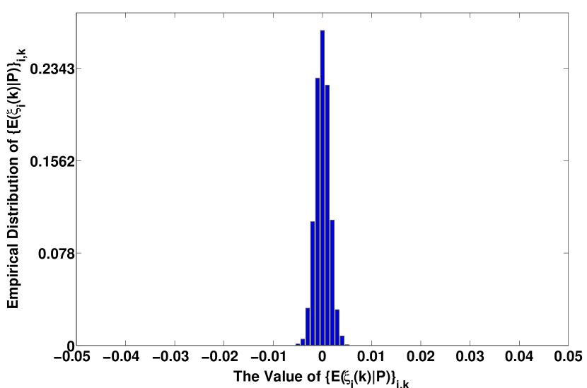
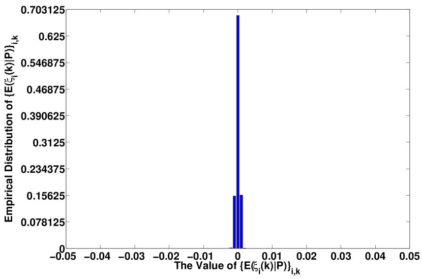
Figure 1: Empirical distribution of $\{E[\xi_{i}(k)|\mathbf{p}]\}_{i,k}$. Left: $L=1,000$; Middle: $L=10,000$; Right: $L=100,000$.

Remark 3

We give some remarks comparing the convergence conditions of conventional IWF and A-IWF under uncertainty. From [16] (Chapter 12, Th. 12.2.1–12.2.5) we see that the condition $\lim_{t\to\infty}||{\mbox{\boldmath$\epsilon$}}^{t}||=0$ in Theorem 2 is sufficient and necessary for the conventional IWF to converge to the fixed point without performing averaging. However, the conventional IWF diverges under condition $\sum_{t=1}^{\infty}\alpha_{t}||{\mbox{\boldmath$\epsilon$}}^{t}||<\infty$ in Theorem 1, because this condition is not equivalent to $\lim_{t\to\infty}||{\mbox{\boldmath$\epsilon$}}^{t}||=0$. Moreover, from Th. 12.2.5 in [16], under the assumption in Theorem 3, the conventional IWF produces a sequence that finally stays in a ball around the fixed point. However, the radius of such ball is increasing with $\frac{\max_{t}{||{\mbox{\boldmath$\xi$}}^{t}||}}{1-\beta}$. Notice that in this case $||{\mbox{\boldmath$\xi$}}^{t}||$ needs not to be decreasing, thus the maximum possible error of the conventional IWF may be large (consider when $\beta$ is close to $1$).

III Simulation Results

In this section we conduct three experiments to demonstrate the properties of the A-IWF algorithm.

III-A Performance with Estimation Error

We simulate a network with $10$ randomly located users, and $64$ channels. We choose the noise to be a zero mean Gaussian random variable as $\epsilon^{t}_{i}(k)\sim N(0,var^{t}_{i}(k))$; we choose the $IER$ for all the users on all the channels to be $IER^{t}_{i}(k)=20dB,~{}15dB$; we choose the channel gains $\{|H_{i,j}(k)|^{2}\}$ randomly and appropriately such that $\rho({\mbox{\boldmath$\Upsilon$}})<1$ is satisfied; we choose $\alpha_{t}=\frac{1}{t+1}$. For ease of demonstration, different algorithms are examined with the same starting points.

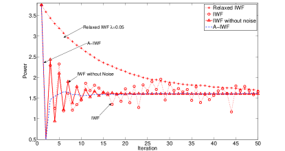
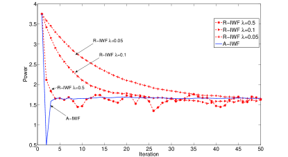
Figure 2: Comparison of the output for different algorithms, IER=20dB.

In Fig. 2, we show the power output produced by various algorithms of a particular user on a particular channel, with $IER=20dB$. It is clear that in the presence of estimation error, the IWF algorithm produces a sequence of noisy power profiles which exhibits no sign of convergence. We also show the performance of IWF algorithm without estimation error, for the purpose of comparison. It is seen that the A-IWF algorithm converges to the unique NE predicted by the IWF (without estimation error) quickly. In Fig. 2, we also show the output of the R-IWF algorithm with various values of $\lambda$. We observe that when $\lambda$ is large, the output is still noisy, while when $\lambda$ is small, the convergence is slow. The point is that the choice of $\lambda$ is important for the performance of R-IWF, but it is difficult to correctly choose $\lambda$ to guarantee both robustness and fast convergence. In Fig. 4, we compare the selected power profiles of R-IWF and A-IWF when $IER=15dB$.

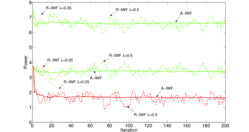
Figure 3: Comparison of different algorithms, IER=15dB.

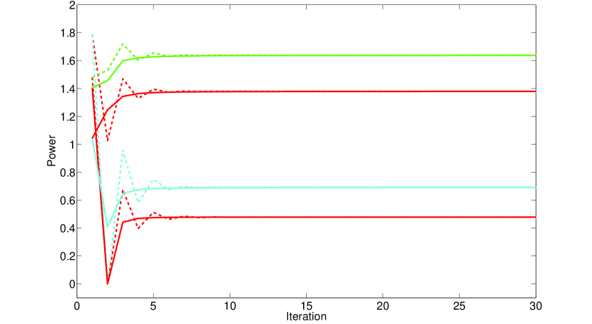
Figure 4: Comparison of convergence speed of IWF and A-IWF.

III-B Performance with Strong Interference

As stated above, the convergence of the IWF in ideal situations usually dependes on the weak interference condition. It is observed that in the system with strong interference, IWF algorithm diverges [8]. In the following simulation, we demonstrate several scenarios in which the IWF diverges, but the A-IWF algorithm converges. The purpose of these simulations is to argue that the A-IWF may need weaker conditions for convergence.

Consider the following scenario of strong interference (example $5$ in [8]). Suppose there are $3$ users and $2$ channels in the system, with channel matrices $\mathbf{H}(k)$ expressed as follows:

$${\tiny\mathbf{H}(1)=\mathbf{H}(2)=\left(\begin{array}[]{ccc}1&0&2\\ 2&1&0\\ 0&2&1\end{array}\right)}$$ (15)

where each element of the matrix $\mathbf{H}(k)$ is defined as $[\mathbf{H}(k)]_{i,j}\triangleq|H_{i,j}(k)|^{2}$. Set the noise power on channel $1$ to be $\sigma^{2}$, the noise on channel $2$ set to be $\sigma^{2}+\bar{p}_{i}$, with $\bar{p}_{i}=10$, for all $i\in\mathcal{N}$. There is a unique NE of this game, in which each user allocates two-thirds of its power to channel $1$ and the rest to channel $2$. The left hand side part of Fig. 5 shows the power profiles of user $1$ on channel $1$ that are produced by different algorithms (with the same starting point). It is seen that the IWF algorithm oscillates, while the A-IWF algorithm converges quickly. Similar results are obtained in the right hand side part of Fig. 5 with the following settings:

$$\tiny\mathbf{H}(1)=\left(\begin{array}[]{ccc}1&2&4\\ 4&1&2\\ 2&4&1\end{array}\right),~{}\mathbf{H}(2)=\left(\begin{array}[]{ccc}2&3&5\\ 3&2&5\\ 5&3&2\end{array}\right)$$ (22)

and the noise power on both channels set to be the same. We observe again that the performance of R-IWF algorithm is very sensitive to the choice of $\lambda$: when $0.6\leq\lambda\leq 1$, the output oscillates; when $0\leq\lambda\leq 0.5$, the output converges, with larger $\lambda$ for faster convergence. However, it is not clear what rules one should follow in general to select such critical parameter.

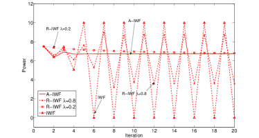
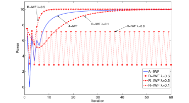
Figure 5: Convergence properties of difference algorithms in strong interference channels.

III-C Convergence In Ideal Cases

Questions may arise as to how does the A-IWF perform in situations when the water-filling solution in (1) can be carried out accurately. As shown in [4], the IWF algorithm converges linearly in this ideal scenario. Theoretically, we can only show that A-IWF converges sublinearly in ideal scenario, i.e., $\lim_{t\to\infty}\frac{||\mathbf{p}^{t+1}-\mathbf{p}^{*}||}{||\mathbf{p}^{t}-\mathbf{p}^{*}||}=1$. However, we observe in various randomly generated channel gains and random starting points of the algorithms, that the A-IWF algorithm seems to always converge as fast as the IWF algorithm. Fig. 4 shows such an instance of this experiment. In this figure, we compare the power output of selected users on selected channels (in a network with 10 users and 64 channels) generated by the IWF and the A-IWF. It takes less than $10$ iterations before two algorithms agree with each other. Note that the dotted lines represent the output of the IWF algorithms and the solid lines represent the output of the A-IWF algorithm.

IV Conclusion

In this correspondence, we proposed an extension to the IWF algorithm which is more robust and has better convergence properties. We proved that the proposed algorithm converges w. p. 1 under suitable assumptions. We argue that this algorithm is indeed robust against time-varying estimation error of the power of interference plus noise that is needed for the computation of the IWF computation. We also show by simulation that the proposed algorithm converges when strong interferences are present in the communication channel, a scenario in which the IWF algorithm diverges. An interesting future research topic is to develop a possibly more general condition for the convergence of the proposed algorithm.

Appendix A Proof of Lemma 1

Proof:

Define $\bar{\mathbf{H}}_{j,i}=diag(|\bar{H}_{j,i}(1)|^{2},\cdots,|\bar{H}_{j,i}(K)|^{2})$; define $\mathbf{IPN}_{i}=\left[IPN_{i}(1),\cdots,IPN_{i}(K)\right]^{\intercal}$, and define $\widehat{\mathbf{IPN}}_{i}$ similarly. From Corollary 3 of [4], we have that the water-filling operator ${\mbox{\boldmath$\Phi$}}_{i}(\mathbf{p}_{-i})$ can be expressed as the projection of $-\mathbf{IPN}_{i}$ onto the space $\mathcal{P}_{i}$, i.e., ${\mbox{\boldmath$\Phi$}}_{i}(\mathbf{p}_{-i})=\left[-\mathbf{IPN}_{i}\right]_{\mathcal{P}_{i}}.$ Similarly, we have that $\widehat{{\mbox{\boldmath$\Phi$}}}_{i}(\mathbf{p}_{-i})=\left[-\widehat{\mathbf{IPN}}_{i}\right]_{\ \mathcal{P}_{i}}$. Consequently, we have:

$$||\widehat{{\mbox{\boldmath$\Phi$}}}_{i}(\mathbf{p}^{1}_{-i})-{{\mbox{\boldmath$\Phi$}}}_{i}(\mathbf{p}^{2}_{-i})||_{2}\stackrel{{\scriptstyle(a)}}{{\leq}}||-\sum_{j\neq i}\bar{\mathbf{H}}_{j,i}\mathbf{p}^{1}_{j}-{\mbox{\boldmath$\epsilon$}}_{i}+\sum_{j\neq i}\bar{\mathbf{H}}_{j,i}\mathbf{p}^{2}_{j}||_{2}$$

$$\leq\sum_{j\neq i}||\bar{\mathbf{H}}_{j,i}||_{2}||\mathbf{p}^{1}_{j}-\mathbf{p}^{2}_{j}||_{2}+||{\mbox{\boldmath$\epsilon$}}_{i}||_{2}$$

$$\stackrel{{\scriptstyle(b)}}{{=}}\sum_{j\neq i}\left(\max_{k}|\bar{{H}}_{j,i}(k)|^{2}\right)||\mathbf{p}^{1}_{j}-\mathbf{p}^{2}_{j}||_{2}+||{\mbox{\boldmath$\epsilon$}}_{i}||_{2},~{}\forall~{}i\in\mathcal{N}$$ (23)

where $(a)$ is because of the non-expansiveness of the projection operator under Euclidean norm; $(b)$ is due to the fact that the 2-norm of a diagonal matrix equals to the maximum absolute value of its diagonal elements. Define ${e}_{{\mbox{\boldmath$\Phi$}}_{i}}\triangleq||\widehat{{\mbox{\boldmath$\Phi$}}}_{i}(\mathbf{p}^{1}_{-i})-{{\mbox{\boldmath$\Phi$}}}_{i}(\mathbf{p}^{2}_{-i})||_{2}$, ${e}_{i}\triangleq||\mathbf{p}^{1}_{i}-\mathbf{p}^{2}_{i}||_{2}$, and let $\mathbf{e}_{{\mbox{\boldmath$\Phi$}}}\triangleq\left[{e}_{{\mbox{\boldmath$\Phi$}}_{1}},\cdots,{e}_{{\mbox{\boldmath$\Phi$}}_{N}}\right]^{\intercal}$, $\mathbf{e}\triangleq\left[{e}_{1},\cdots,{e}_{N}\right]^{\intercal}$, and $\mathbf{e}_{{\mbox{\boldmath$\epsilon$}}}\triangleq\left[||{\mbox{\boldmath$\epsilon$}}_{1}||_{2},\cdots,||{\mbox{\boldmath$\epsilon$}}_{N}||_{2}\right]^{\intercal}$.

In order to proceed, we define the vector weighted maximum norm [15] as:

$$||\mathbf{x}||^{\mathbf{w}}_{\infty,vec}\triangleq\max_{i}\frac{|x_{i}|}{w_{i}},~{}\mathbf{w}>\mathbf{0},\mathbf{x}\in\mathbb{R}^{N}$$ (24)

and the matrix weighted maximum norm as:

$$||\mathbf{A}||^{\mathbf{w}}_{\infty,mat}\triangleq\max_{i}\frac{1}{w_{i}}\sum_{j=1}^{N}{|[\mathbf{A}]_{i,j}|}w_{j},~{}\mathbf{w}>\mathbf{0},\mathbf{A}\in\mathbb{R}^{N\times N}.$$ (25)

Notice, that from the definition of norm $||.||^{\mathbf{w}}_{\infty,vec}$, $||.||^{\mathbf{w}}_{\infty,mat}$ and the block-maximum norm, we have the following equivalence:

$$||\mathbf{e}||^{\mathbf{w}}_{\infty,vec} =\max_{i}\frac{|{e}_{i}|}{w_{i}}=\max_{i}\frac{||\mathbf{p}_{i}^{1}-\mathbf{p}_{i}^{2}||}{w_{i}}=||\mathbf{p}^{1}-\mathbf{p}^{2}||^{\mathbf{w}}_{2,block}$$

$$||\mathbf{e}_{{\mbox{\boldmath$\Phi$}}}||^{\mathbf{w}}_{\infty,vec} =\max_{i}\frac{|e_{{\mbox{\boldmath$\Phi$}}_{i}}|}{w_{i}}=||\widehat{{\mbox{\boldmath$\Phi$}}}(\mathbf{p}^{1})-{\mbox{\boldmath$\Phi$}}(\mathbf{p}^{2})||^{\mathbf{w}}_{2,block}$$

$$||\mathbf{e}_{{\mbox{\boldmath$\epsilon$}}}||^{\mathbf{w}}_{\infty,vec} =\max_{i}\frac{||{\mbox{\boldmath$\epsilon$}}_{i}||_{2}}{w_{i}}=||{\mbox{\boldmath$\epsilon$}}||^{\mathbf{w}}_{2,block}.$$ (26)

The set of $N$ inequalities in (23) can be concisely written in vector form as ($\Upsilon$ is defined in (9)): $\mathbf{e}_{{\mbox{\boldmath$\Phi$}}}\leq{\mbox{\boldmath$\Upsilon$}}\mathbf{e}+\mathbf{e}_{{\mbox{\boldmath$\epsilon$}}}.$ Applying vector weighted maximum norm to this inequality results in:

$$||\mathbf{e}_{{\mbox{\boldmath$\Phi$}}}||^{\mathbf{w}}_{\infty,vec} \leq||{\mbox{\boldmath$\Upsilon$}}||^{\mathbf{w}}_{\infty,mat}||\mathbf{e}||^{\mathbf{w}}_{\infty,vec}+||\mathbf{e}_{{\mbox{\boldmath$\epsilon$}}}||^{\mathbf{w}}_{\infty,vec}$$

$$=||{\mbox{\boldmath$\Upsilon$}}||^{\mathbf{w}}_{\infty,mat}||\mathbf{p}^{1}-\mathbf{p}^{2}||^{\mathbf{w}}_{2,block}+||{{\mbox{\boldmath$\epsilon$}}}||^{\mathbf{w}}_{2,block}.$$ (27)

Arguing similarly as the derivation of the Proposition 2 of [4] by using (26) and (27) we have:

$$||\widehat{{\mbox{\boldmath$\Phi$}}}(\mathbf{p}^{1})-{\mbox{\boldmath$\Phi$}}(\mathbf{p}^{2})||^{\mathbf{w}}_{2,block}$$

$$=||\mathbf{e}_{{\mbox{\boldmath$\Phi$}}}||^{\mathbf{w}}_{\infty,vec}\leq||{\mbox{\boldmath$\Upsilon$}}||^{\mathbf{w}}_{\infty,mat}||\mathbf{p}^{1}-\mathbf{p}^{2}||_{2,block}^{{\mathbf{w}}}+||{\mbox{\boldmath$\epsilon$}}||_{2,block}^{{\mathbf{w}}}.$$ (28)

Since $\Upsilon$ is a non-negative matrix, from [15] Corollary 6.1, we have that there exists a $\bar{{\mathbf{w}}}$ such that $\rho({\mbox{\boldmath$\Upsilon$}})<1\Longleftrightarrow||{\mbox{\boldmath$\Upsilon$}}||_{\infty,mat}^{\bar{{\mathbf{w}}}}<1.$ Consequently, we conclude that if $\rho({\mbox{\boldmath$\Upsilon$}})<1$, then there must exists a $\beta\in(0,1)$ and a positive vector $\bar{{\mathbf{w}}}$ that satisfy (10). ∎

Appendix B Proof of Theorem 1

Proof:

Starting from an arbitrary initial point $\mathbf{p}^{0}\in\mathcal{P}$, the magnitude of the difference between $\mathbf{p}^{1}$ and the fixed point $\mathbf{p}^{\ast}$ can be expressed as:

$$||\mathbf{p}^{1}-\mathbf{p}^{*}|| =||(1-\alpha_{0})\mathbf{p}^{0}+\alpha_{0}\widehat{{\mbox{\boldmath$\Phi$}}}(\mathbf{p}^{0})-{\mbox{\boldmath$p$}}^{*}||$$

$$\leq||(1-\alpha_{0})(\mathbf{p}^{0}-\mathbf{p}^{*})||+\left|\left|\alpha_{0}\left(\widehat{{\mbox{\boldmath$\Phi$}}}(\mathbf{p}^{0})-{{\mbox{\boldmath$\Phi$}}}(\mathbf{p}^{*})\right)\right|\right|$$

$$\stackrel{{\scriptstyle(i)}}{{\leq}}(1-\alpha_{0})||\mathbf{p}^{0}-\mathbf{p}^{*}||+\alpha_{0}\beta||\mathbf{p}^{0}-\mathbf{p}^{*}||+||\alpha_{0}{\mbox{\boldmath$\epsilon$}}^{0}||$$

$$=\left(1-\alpha_{0}(1-\beta)+\frac{||\alpha_{0}{\mbox{\boldmath$\epsilon$}}^{0}||}{||{\mbox{\boldmath$p$}}^{0}-{\mbox{\boldmath$p$}}^{*}||}\right)||{\mbox{\boldmath$p$}}^{0}-{\mbox{\boldmath$p$}}^{*}||$$ (29)

where $(i)$ is from Lemma 1. Let us denote $\mu_{t}\triangleq(1-\alpha_{t}(1-\beta))$. From (5) and (6), clearly we have $\alpha_{0}=1$ and $\alpha_{t}\leq 1$, which implies $\mu_{0}\leq\mu_{t}~{}\forall~{}t$. By induction, we show that in general:

$$||{\mbox{\boldmath$p$}}^{T}-{\mbox{\boldmath$p$}}^{*}||\leq\Big{(}\prod_{t=0}^{T-1}\mu_{i}+\frac{\sum_{t=0}^{T-1}\left(\prod_{j=t}^{T-1}\mu_{j}\right)||\alpha_{t}{\mbox{\boldmath$\epsilon$}}^{t}||}{\mu_{0}||{\mbox{\boldmath$p$}}^{0}-{\mbox{\boldmath$p$}}^{*}||}\Big{)}||{\mbox{\boldmath$p$}}^{0}-{\mbox{\boldmath$p$}}^{*}||.$$ (30)

Clearly from (29) at time $T=1$, (30) is true. Suppose at time $T$, (30) is true. At time $T+1$, we have:

$$||{\mbox{\boldmath$p$}}^{T+1}-{\mbox{\boldmath$p$}}^{*}||\leq(1-\alpha_{T})||{\mbox{\boldmath$p$}}^{T}-{\mbox{\boldmath$p$}}^{*}||+\alpha_{T}\beta||{\mbox{\boldmath$p$}}^{T}-{\mbox{\boldmath$p$}}^{*}||+||\alpha_{T}{\mbox{\boldmath$\epsilon$}}^{T}||$$

$$\leq\Big{(}\prod_{t=0}^{T}\mu_{i}+\frac{\sum_{t=0}^{T-1}\left(\prod_{j=t}^{T}\mu_{j}\right)||\alpha_{t}{\mbox{\boldmath$\epsilon$}}^{t}||}{\mu_{0}||{\mbox{\boldmath$p$}}^{0}-{\mbox{\boldmath$p$}}^{*}||}+\frac{||\alpha_{T}{\mbox{\boldmath$\epsilon$}}^{T}||}{||{\mbox{\boldmath$p$}}^{0}-{\mbox{\boldmath$p$}}^{*}||}\Big{)}||{\mbox{\boldmath$p$}}^{0}-{\mbox{\boldmath$p$}}^{*}||$$

$$\leq\Big{(}\prod_{t=0}^{T}\mu_{i}+\frac{\sum_{t=0}^{T}\left(\prod_{j=t}^{T}\mu_{j}\right)||\alpha_{t}{\mbox{\boldmath$\epsilon$}}^{t}||}{\mu_{0}||{\mbox{\boldmath$p$}}^{0}-{\mbox{\boldmath$p$}}^{*}||}\Big{)}||{\mbox{\boldmath$p$}}^{0}-{\mbox{\boldmath$p$}}^{*}||.$$ (31)

Note that in the last inequality, we have used the fact that $\mu_{t}\geq\mu_{0}$, and $\frac{||\alpha_{T}{\mbox{\boldmath$\epsilon$}}^{T}||}{||{\mbox{\boldmath$p$}}^{0}-{\mbox{\boldmath$p$}}^{*}||}\leq\frac{\mu_{T}||\alpha_{T}{\mbox{\boldmath$\epsilon$}}^{T}||}{\mu_{0}||{\mbox{\boldmath$p$}}^{0}-{\mbox{\boldmath$p$}}^{*}||}$. From the assumption $\sum_{t=1}^{\infty}\alpha_{t}||{\mbox{\boldmath$\epsilon$}}^{t}||<\infty,~{}\textrm{w. p. 1}$, there must exist some constant $0<b<\infty$ such that:

$$\lim_{T\to\infty}\sum_{t=1}^{T}||\alpha_{t}{\mbox{\boldmath$\epsilon$}}^{t}||\leq b<\infty~{}\textrm{w. p. 1}.$$ (32)

In the following, we show $\lim_{T\to\infty}\sum_{t=0}^{T-1}\left(\prod_{j=t}^{T-1}\mu_{j}\right)||\alpha_{t}{\mbox{\boldmath$\epsilon$}}^{t}||=0~{}$ w. p. 1.

First note that we have $\lim_{T\to\infty}\prod_{t=0}^{T}\mu_{t}=0$, because:

$$\lim_{T\to\infty}\log\Big{(}\prod_{t=0}^{T}\mu_{t}\Big{)} =\lim_{T\to\infty}\sum_{t=0}^{T}\log\Big{(}1+(-\alpha_{t}(1-\beta))\Big{)}\stackrel{{\scriptstyle(i)}}{{}}$$

$$\leq\lim_{T\to\infty}(1-\beta)\sum_{t=0}^{T}-\alpha_{t}\stackrel{{\scriptstyle(ii)}}{{=}}-\infty$$ (33)

where $(i)$ is because $-1<-\alpha_{t}(1-\beta)$ and the fact $\log(1+x)\leq x,\forall~{}x>-1$, $(ii)$ is because (6) and $\beta<1$. Clearly (33) implies $\lim_{T\to\infty}\prod_{t=0}^{T}\mu_{t}=0$. Thus for any $\delta>0$, and a fixed $T$ there exists $\hat{T}(T,\delta)>T$ such that:

$$\prod_{t=T}^{N-1}\mu_{t}\leq\frac{\delta}{2b},~{}\forall~{}N\geq\hat{T}(T,\delta).$$ (34)

From (32) we have that for any $\delta>0$, there exists $T(\delta)$ such that:

$$\sum_{t=T}^{\infty}||\alpha_{t}{\mbox{\boldmath$\epsilon$}}^{t}||\leq\frac{\delta}{2},~{}\forall~{}T\geq T(\delta),~{}\textrm{w. p. 1}.$$ (35)

Then we have that for all $N>\max\left\{T(\delta),\hat{T}(T(\delta),\delta)\right\}=\hat{T}(T(\delta),\delta)$:

$$\sum_{t=0}^{N}\big{(}\prod_{j=t}^{N-1}\mu_{j}\big{)}||\alpha_{t}{\mbox{\boldmath$\epsilon$}}^{t}||$$

$$=\sum_{t=0}^{T(\delta)}\big{(}\prod_{j=t}^{N-1}\mu_{j}\big{)}||\alpha_{t}{\mbox{\boldmath$\epsilon$}}^{t}||+\sum_{t=T(\delta)+1}^{N}\big{(}\prod_{j=t}^{N-1}\mu_{j}\big{)}||\alpha_{t}{\mbox{\boldmath$\epsilon$}}^{t}||$$

$$\stackrel{{\scriptstyle(i)}}{{\leq}}\sum_{t=0}^{T(\delta)}\big{(}\prod_{j=T(\delta)}^{N-1}\mu_{j}\big{)}||\alpha_{t}{\mbox{\boldmath$\epsilon$}}^{t}||+\frac{\delta}{2}$$

$$\stackrel{{\scriptstyle(ii)}}{{\leq}}\prod_{j=T(\delta)}^{N-1}\mu_{j}\sum_{t=0}^{T(\delta)}||\alpha_{t}{\mbox{\boldmath$\epsilon$}}^{t}||+\frac{\delta}{2}\stackrel{{\scriptstyle(iii)}}{{}}$$

$$\leq\frac{\delta}{2b}b+\frac{\delta}{2}=\delta~{}~{}\textrm{w. p. 1}$$ (36)

where $(i)$ is because (35) and the fact that $\prod_{j=t}^{N-1}\mu_{j}<1$ for all $t\leq N-1$; $(ii)$ is because $\prod_{j=T(\delta)}^{N-1}\mu_{j}$ is independent of $t$; $(iii)$ is because of (32) and (34). Consequently, we have that:

$$\lim_{T\to\infty}\sum_{t=0}^{T-1}\big{(}\prod_{j=t}^{T-1}\mu_{j}\big{)}||\alpha_{t}{\mbox{\boldmath$\epsilon$}}^{t}||=0~{}\textrm{w. p. 1}.$$ (37)

From (30), (37), and $\lim_{T\to\infty}\prod_{t=0}^{T}\mu_{t}=0$, we conclude : $\lim_{t\to\infty}||{\mbox{\boldmath$p$}}^{t}-{\mbox{\boldmath$p$}}^{*}||=0~{}\textrm{w. p. 1}.$ ∎

Appendix C Proof of Theorem 2

Proof:

Due to space limit, we only show the proof for the case that $\alpha_{t}=\frac{1}{t+1}$. The proof for general $\{\alpha_{t}\}$ can be obtained similarly. When taking $\alpha_{t}=\frac{1}{t+1}$, the A-IWF algorithm can be written compactly as: $\mathbf{p}^{T+1}=\frac{1}{T+1}\sum_{t=0}^{T}\widehat{{\mbox{\boldmath$\Phi$}}}(\mathbf{p}^{t})$. We can write:

$$||\mathbf{p}^{T+1}-\mathbf{p}^{*}|| \leq\frac{1}{T+1}\sum_{t=0}^{T}||\widehat{{\mbox{\boldmath$\Phi$}}}(\mathbf{p}^{t})-{{\mbox{\boldmath$\Phi$}}}(\mathbf{p}^{*})||$$

$$\stackrel{{\scriptstyle(i)}}{{\leq}}\frac{\beta}{T+1}\sum_{t=0}^{T}||\mathbf{p}^{t}-\mathbf{p}^{*}||+\frac{1}{T+1}\sum_{t=0}^{T}||{\mbox{\boldmath$\epsilon$}}^{t}||$$ (38)

where $(i)$ is from Lemma 1. Suppose the sequence $\{\mathbf{p}^{t}\}$ does not converge to $\mathbf{p}^{*}$, i.e., $\lim_{T\to\infty}\sup||\mathbf{p}^{T}-\mathbf{p}^{*}||=\delta>0$. Using the Stolz-Cesàro Theorem [17], we have that:

$$\lim_{T\to\infty}\sup\frac{\sum_{t=0}^{T}||\mathbf{p}^{t}-\mathbf{p}^{\ast}||}{T+1}\leq\lim_{T\to\infty}\sup||\mathbf{p}^{T}-\mathbf{p}^{\ast}||=\delta;$$

$$\lim_{T\to\infty}\frac{\sum_{t=0}^{T}||{\mbox{\boldmath$\epsilon$}}^{t}||}{T+1}=\lim_{T\to\infty}||{\mbox{\boldmath$\epsilon$}}^{T}||=0,~{}\textrm{w. p. 1}.$$ (39)

Taking $\lim\sup$ on both sides of (38), we have:

$$\lim_{T\to\infty}\sup||\mathbf{p}^{T+1}-\mathbf{p}^{*}||$$

$$\leq\lim_{T\to\infty}\sup\frac{\beta}{T+1}\sum_{t=0}^{T}||\mathbf{p}^{t}-\mathbf{p}^{*}||+\lim_{T\to\infty}\sup\frac{1}{T+1}\sum_{t=0}^{T}||{\mbox{\boldmath$\epsilon$}}^{t}||$$ (40)

which can be reduced to: $\delta\leq\beta\delta$ by applying (39). This is a contradiction to the fact that $\beta<1$. Then we conclude that $\lim_{T\to\infty}\sup||\mathbf{p}^{T}-\mathbf{p}^{*}||=0$ which in turn implies $\lim_{T\to\infty}||\mathbf{p}^{T}-\mathbf{p}^{*}||=0$. ∎

Appendix D Proof of Theorem 3

Due to space limit, we only show the proof for the case that $\alpha_{t}=\frac{1}{t+1}$. The proof for general $\{\alpha_{t}\}$ can be obtained similarly. We first state a lemma, the proof of which can be found in Appendix E.

Lemma 2

If ${w}^{t+1}=(1-\alpha_{t}){w}^{t}+\alpha_{t}\xi^{t+1}$, and $E[\xi^{t}|\mathcal{F}^{t-1}]=0$, and $E[(\xi^{t})^{2}|\mathcal{F}^{t-1}]=b$ is uniformly bounded, $\{\alpha_{t}\}$ satisfies (6), then we must have $\lim_{t\to\infty}{w}^{t}=0,~{}\textrm{w. p. 1.}$

We are now ready to prove Theorem 3. The A-IWF algorithm can be compactly written as: $\mathbf{p}^{T+1}=\frac{1}{T+1}\sum_{t=0}^{T}\widehat{{\mbox{\boldmath$\Phi$}}}(\mathbf{p}^{t})=\frac{1}{T+1}\sum_{t=0}^{T}{{\mbox{\boldmath$\Phi$}}}(\mathbf{p}^{t})+\mathbf{w}^{T}$, where $\mathbf{w}^{T}\triangleq\frac{1}{T+1}\sum_{t=0}^{T}{\mbox{\boldmath$\xi$}}^{t}=(1-\frac{1}{T+1})\mathbf{w}^{T-1}+\frac{1}{T+1}{\mbox{\boldmath$\xi$}}^{T}$. Note that by applying the results of Lemma 2, we have $\lim_{T\to\infty}\mathbf{w}^{T}=0$. Then the magnitude of difference between $\mathbf{p}^{T+1}$ and the unique fixed point of the mapping ${\mbox{\boldmath$\Phi$}}(.)$ can be expressed as:

$$||\mathbf{p}^{T+1}-\mathbf{p}^{\ast}|| \leq\frac{1}{T+1}\sum_{t=0}^{T}||{{\mbox{\boldmath$\Phi$}}}(\mathbf{p}^{t})-{{\mbox{\boldmath$\Phi$}}}(\mathbf{p}^{\ast})||+||\mathbf{w}^{T}||$$

$$\leq\frac{\beta}{T+1}\sum_{t=0}^{T}||\mathbf{p}^{t}-\mathbf{p}^{\ast}||+||\mathbf{w}^{T}||.$$ (41)

Suppose the sequence $\{\mathbf{p}^{t}\}$ does not converge to $\mathbf{p}^{*}$, then there must exist a $\delta>0$ such that $\lim_{T\to\infty}\sup||\mathbf{p}^{t}-\mathbf{p}^{*}||=\delta$. Using again the Stolz-Cesàro Theorem as in (39), and taking $\lim\sup$ on both sides of (41), we have: $\lim_{T\to\infty}\sup||\mathbf{p}^{T+1}-\mathbf{p}^{\ast}||\leq\lim_{T\to\infty}\sup\frac{\beta}{T+1}\sum_{t=0}^{T}||\mathbf{p}^{t}-\mathbf{p}^{\ast}||+\lim_{T\to\infty}||\mathbf{w}^{T}||.$ This inequality can be reduced to: $\delta\leq\beta\delta$, which contradicts to the fact that $\beta<1$. Thus we conclude that $\lim_{T\to\infty}||\mathbf{p}^{t}-\mathbf{p}^{*}||=0$, and that $\lim_{T\to\infty}\mathbf{p}^{t}=\mathbf{p}^{\ast}$.

Appendix E Proof of Lemma 2

Proof:

We have ${w}^{t+1}={w}^{t}+\alpha_{t}(\xi^{t+1}-{w}^{t})$. Consider the following iteration:

$$({w}^{t+1})^{2} =({w}^{t}+\alpha_{t}(\epsilon^{t+1}-{w}^{t}))^{2}$$

$$=({w}^{t})^{2}+2\alpha_{t}(\xi^{t+1}-{w}^{t}){w}^{t}+\alpha^{2}_{t}(\xi^{t+1}-{w}^{t})^{2}.$$ (42)

Then $E[({w}^{t+1})^{2}|\mathcal{F}^{t}]$ can be expressed as:

$$E[({w}^{t+1})^{2}|\mathcal{F}^{t}]$$

$$=({w}^{t})^{2}_{t}-2\alpha_{t}({w}^{t})^{2}+2\alpha_{t}E[\xi^{t+1}|\mathcal{F}^{t}]{w}^{t}+\alpha^{2}_{t}E[(\xi^{t+1}-{w}^{t})^{2}|\mathcal{F}^{t}]$$

$$=({w}^{t})^{2}-2\alpha_{t}({w}^{t})^{2}+\alpha_{t}^{2}\left(E[(\xi^{t+1})^{2}|\mathcal{F}^{t}]+({w}^{t})^{2}-2{w}^{t}E[\xi^{t+1}|\mathcal{F}^{t}]\right)$$

$$\leq({w}^{t})^{2}-2\alpha_{t}(1-\frac{\alpha_{t}}{2})({w}^{t})^{2}+\alpha^{2}_{t}b.$$ (43)

Notice that the term $2\alpha_{t}(1-\frac{\alpha_{t}}{2})({w}^{t})^{2}\geq 0$ because $0<\alpha_{t}\leq 1$. We see that $\lim_{T\to\infty}\sum_{t=0}^{T}\alpha^{2}_{t}b<\infty$ because $\sum_{t=1}^{\infty}\alpha^{2}_{t}<\infty$. In order to proceed, we define the notion of a non-negative almost-supermartingale [18]. Let $z_{t}$, $\beta_{t}$, $\xi_{t}$ and $\zeta_{t}$ be non-negative $\mathcal{F}^{t}$ measurable random variables. The sequence $\{z_{t}\}$ is called non-negative almost-supermartingale if $E[z_{t+1}|\mathcal{F}^{t}]\leq(1+\beta_{t})z_{t}+\xi_{t}-\zeta_{t}.$ From Theorem 1 of [18], we have $\lim_{t\to\infty}z_{t}$ exists and is finite and $\sum_{t=1}^{\infty}\zeta_{t}<\infty$ w. p. 1 if $\left\{\sum_{t=1}^{\infty}\beta_{t}<\infty,\sum_{t=1}^{\infty}\xi_{t}<\infty\right\}$.

Now it is clear that the sequence $\{({w}^{t})^{2}\}_{t=0}^{\infty}$ is a non-negative almost-supermartingale, and according to the above mentioned theorem we have the following results: 1) $\{({w}^{t})^{2}\}_{t=0}^{\infty}$ converges; 2) $\sum_{t=1}^{T}\alpha_{t}(1-\frac{\alpha_{t}}{2})({w}^{t})^{2}<\infty$ w. p. 1. The second result implies that $\lim_{T\to\infty}\sum_{t=1}^{T}\alpha_{t}({w}^{t})^{2}<\infty$. Combined with the fact that $\sum_{t=0}^{\infty}\alpha_{t}=\infty$ and $\lim_{t\to\infty}\alpha_{t}=0$, we have that $\lim\inf_{t\to\infty}({w}^{t})^{2}={0}$. Moreover, we know from the first result that the sequence $\{({w}^{t})^{2}\}_{t=0}^{\infty}$ converges, then it must converge to ${0}$. ∎

References

- [1] W. Yu, G. Ginis, and J. M. Cioffi, “Distributed multiuser power control for digital subscriber lines,” IEEE Journal on Selected Areas in Communications, vol. 20, no. 5, pp. 1105–1115, 2002.
- [2] G. Scutari, D. P. Palomar, and S. Barbarossa, “Optimal linear precoding strategies for wideband noncooperative systems based on game theory – part I: Nash equilibria,” IEEE Trans. on Signal Processing, vol. 56, no. 3, pp. 1230–1249, 2008.
- [3] F. Wang, M. Krunz, and S. G. Cui, “Price-based spectrum management in cognitive radio networks,” IEEE Journal of Selected Topics in Signal Processing, vol. 2, no. 1, pp. 74–87, 2008.
- [4] G. Scutari, D. P. Palomar, and S. Barbarossa, “Optimal linear precoding strategies for wideband noncooperative systems based on game theory – part II: Algorithms,” IEEE Trans. on Signal Processing, vol. 56, no. 3, pp. 1250–1267, 2008.
- [5] G. Scutari, D. P. Palomar, and S. Barbarossa, “Asynchronous iterative water-filling for Gaussian frequency-selective interference channels,” IEEE Transactions on Information Theory, vol. 54, no. 7, pp. 2868–2878, 2008.
- [6] Z-. Q. Luo and J-.S. Pang, “Analysis of iterative waterfilling algorithm for multiuser power contorl in digital subscriber lines,” EURASIP Journal on Applied Signal Processing, vol. 2006, pp. 1–10, 2006.
- [7] K. W. Shum, K. K. Leung, and C. W. Sung, “Convergence of iterative waterfilling algorithm for Gaussian interference channels,” IEEE Journal on Selected Area in Communications, vol. 25, pp. 1091–1100, 2007.
- [8] A. Leshem and E. Zehavi, “Game theory and the frequency selective interference channel,” IEEE Signal Processing Magazine, vol. 26, no. 5, pp. 28–40, 2009.
- [9] T. R. Benedict and T. T. Soong, “The joint estimation of signal and noise from the sum evelope,” IEEE Transactions on Information Theory, vol. 13, no. 3, pp. 447–454, 1967.
- [10] D. R. Pauluzzi and N. C. Beaulieu, “A comparison of SNR estimation techniques for the AWGN channel,” IEEE Transactions on Communications, vol. 48, no. 10, pp. 1681–1691, 2000.
- [11] P. Setoodeh and S. Haykin, “Robust transmit powercontrol for cognitive radio,” Proceedings of IEEE, pp. 915–939, 2009.
- [12] R. H. Gohary and T. J. Willink, “Robust IWFA for open-spectrum communications,” IEEE Trans. On Signal Process., vol. 57, no. 12, pp. 4964–4970, 2009.
- [13] Y. Cheng and V. K. N. Lau, “Distributive power control algorithm for multicarrier interference network over time-varying fading channels–tracking performance analysis and optimization,” IEEE Transactions on Signal Processing, vol. 58, no. 9, pp. 4750–4760, 2010.
- [14] W. R. Mann, “Mean value methods in iteration,” in Proc. Amer. Math.Soc., 1953, pp. 506–510.
- [15] D. P. Bertsekas and J. N. Tsitsiklis, Parallel and Distributed Computation: Numerical Methods, Athena Scientific, 1997.
- [16] J. M. Ortega and W. C. Rheinboldt, Iterative Solution of Nonlinear Equations in Several Variables, Academic Press, 1972.
- [17] M. Muresan, A Concrete Approach to Classical Analysis, Springer, 2008.
- [18] H. Robbins and D. Siegmund, A Convergence Theorem for Non-Negative Almost Supermartingales and Some Applications, Optimizing Methods in Statistics. Academic Press, New York, 1971.