Convex Hull of Points Lying on Lines in $o(n\log{n})$ Time after Preprocessing

Abstract

Motivated by the desire to cope with data imprecision [31], we study methods for taking advantage of preliminary information about point sets in order to speed up the computation of certain structures associated with them.

In particular, we study the following problem: given a set $L$ of $n$ lines in the plane, we wish to preprocess $L$ such that later, upon receiving a set $P$ of $n$ points, each of which lies on a distinct line of $L$, we can construct the convex hull of $P$ efficiently. We show that in quadratic time and space it is possible to construct a data structure on $L$ that enables us to compute the convex hull of any such point set $P$ in $O(n\alpha(n)\log^{*}n)$ expected time. If we further assume that the points are “oblivious” with respect to the data structure, the running time improves to $O(n\alpha(n))$. The same result holds when $L$ is a set of line segments (in general position). We present several extensions, including a trade-off between space and query time and an output-sensitive algorithm. We also study the “dual problem” where we show how to efficiently compute the $(\leq k)$-level of $n$ lines in the plane, each of which is incident to a distinct point (given in advance).

We complement our results by $\Omega(n\log{n})$ lower bounds under the algebraic computation tree model for several related problems, including sorting a set of points (according to, say, their $x$-order), each of which lies on a given line known in advance. Therefore, the convex hull problem under our setting is easier than sorting, contrary to the “standard” convex hull and sorting problems, in which the two problems require $\Theta(n\log{n})$ steps in the worst case (under the algebraic computation tree model).

1 Introduction

Most studies in computational geometry rely on an unspoken assumption: whenever we are given a set of input points, their precise locations are available to us. Nowadays, however, the input is often obtained via sensors from the real world, and hence it comes with an inherent imprecision. Accordingly, an increasing effort is being devoted to achieving a better understanding of data imprecision and to developing tools to cope with it (see, e.g., [31] and the references therein). The notion of imprecise data can be formalized in numerous ways [31, 24, 33]. We consider a particular setting that has recently attracted considerable attention [8, 20, 25, 30, 32, 34]. We are given a set of planar regions, each of which represents an estimate about an input point, and the exact coordinates of the points arrive some time later and need to be processed quickly. This situation could occur, e.g., during a two-phase measuring process: first the sensors quickly obtain a rough estimate of the data, and then they invest considerably more time to find the precise locations. This raises the necessity to preprocess the preliminary (imprecise) locations of the points, and store them in an appropriate data structure, so that when the exact measurements of the points arrive we can efficiently compute a pre-specified structure on them. In settings of this kind, we assume that for each input point its corresponding region is known (note that by this assumption we also avoid a point-location overhead). In light of the applications, this is a reasonable assumption, and it can be implemented by, e.g., encoding this information in the ordering of $P$.

Related work

Data imprecision. Previous work has mainly focused on computing a triangulation for the input points. Held and Mitchell [25] were the first to consider this framework, and they obtained optimal bounds for preprocessing disjoint unit disks for point set triangulations, a result that was later generalized by van Kreveld et al. [30] to arbitrary disjoint polygonal regions. For Delaunay triangulations, Löffler and Snoeyink [34] obtained an optimal result for disjoint unit disks (see also [20, 32]), which was later simplified and generalized by Buchin et al. [8] to fat and possibly intersecting regions. If $n$ is the number of input regions, the preprocessing phase typically takes $O(n\log n)$ time and yields a linear size data structure; the time to find the structure on the exact points is usually linear or depends on the complexity (and the fatness) of the input regions.

Since the convex hull can be easily extracted from the Delaunay triangulation in linear time, the same bounds carry over. However, once the regions are not necessarily fat, the techniques in [8, 34] do not yield the aforementioned bounds anymore. In particular, if the regions consist of lines or line segments, one cannot hope (under certain computational models) to construct the Delaunay triangulation of $P$ in time $o(n\log n)$, regardless of preprocessing (see [22] and Section 4). Nevertheless, if we are less ambitious and just wish to compute the convex hull of $P$, we can achieve better performance, as our main result shows.

Convex hull. Computing the convex hull of a planar $n$-point set is perhaps the most fundamental problem in computational geometry, and there are many algorithms available [6, 37]. All these algorithms require $\Theta(n\log n)$ steps, which is optimal in the algebraic computation tree model [5]. However, there are numerous ways to exploit additional information to improve this bound. For example, if the points are sorted along any fixed direction, Graham’s scan takes only linear time [6]. If we know that there are only $h$ points on the hull, the running time reduces to $O(n\log h)$ [28, 1]. If the points constitute the vertices of a given polygonal chain, the complexity again reduces to linear [36]. Our work shows another setting in which additional information can be used to circumvent the theoretic lower bound.

Another somewhat related problem (albeit conceptually different) is the kinetic convex hull problem, where we are given $n$ points which move continuously in the plane, and the goal is to maintain their convex hull over time. Kinetic data structures have been introduced by Basch et al. [4] and received considerable attention in follow-up studies (see, e.g., [2] and the references therein). When the trajectories of the points are lines, our problem can be interpreted as a (perhaps, extended and intricate) variant of the kinetic convex hull problem. Indeed, if the goal is to preprocess the linear trajectories such that the convex hull can be reported efficiently at any given time $t$, our algorithm applies (in which case the exact set of points $P$ consists of their positions at time $t$) and yields a relatively simple solution. Nevertheless, our problem is more intricate than the kinetic convex hull problem for linear trajectories, as in our scenario there is no continuous motion that enables us to have a better control on the exact set of points (once they arrive).

Our results. We show that under a mild assumption (see Section 2.2) we can preprocess the input lines $L$ such that given any set $P$ of points, each of which lies on a distinct line of $L$, the convex hull $\operatorname{CH}(P)$ can be computed in expected time $O(n\alpha(n))$, where $\alpha(\cdot)$ is the (slowly growing) inverse Ackermann function [41, Chapter 2.1]; the expected running time is $O(n\alpha(n)\log^{*}n)$ without this assumption. Our data structure has quadratic preprocessing time and storage, and the convex hull algorithm is based on a batched randomized incremental construction similar to Seidel’s tracing technique [40]. As part of the construction, we repeatedly trace the zone of (the boundary of) an intermediate hull in the arrangement of the input lines (see below for the definitions). The fact that the complexity of the zone is only $O(n\alpha(n))$ [7, 41], and that it can be computed in the same asymptotic time bound (after having the arrangement at hand), is a key property of our solution. The analysis also applies when $L$ is a set of line segments, and yields the same result.

We also show that the analogous problem in which we just wish to sort the points according to their $x$-order imposes algebraic computation trees of depth $\Omega(n\log{n})$. Hence, in our setting convex hull computation is strictly easier than sorting, contrary to the “standard” (unconstrained) model, in which both problems are equivalent in terms of hardness (see, e.g., [6]). Our results can be extended with similar bounds to several related problems, such as determining the width and diameter of $P$, as well as time-space trade-offs and designing an output-sensitive algorithm. Unfortunately, already for the closest pair problem a preprocessing of the regions is unlikely to decrease the query time to $o(n\log{n})$, demonstrating once again the delicate nature of our setting.

In Section 3 we study a generalization of the problem under the dual setting. Specifically, we wish to preprocess a planar $n$-point set $P$ such that given an integer $k$ and a set $L$ of lines, each of which is incident to a distinct point of $P$, we can find the “$(\leq k)$-level” in the arrangement of $L$ efficiently. We show a randomized construction whose expected running time is $O(n\alpha(n)+nk)$ under a mild assumption, and $O(n\alpha(n)\log^{*}n+nk)$ without this assumption. As above, our data structure has quadratic preprocessing time and storage. This improves over the $O(n\log n+nk)$ time algorithms in the traditional model [10, 23], as long as $k=o(\log n)$. Our approach is a non-trivial extension of the technique presented in Section 2, incorporated with the algorithms of Chan [10] and Everett et al. [23], as well as the Clarkson-Shor technique [16].

The quadratic preprocessing time and storage might seem disappointing. However, a related lower bound by Ali Abam and de Berg [2] from the study of kinetic convex hulls (albeit providing a weaker evidence) suggests that quadratic space might be necessary, and that only relatively weak time-space trade-offs (as in Section 2.3) are possible in this model (see the discussion in Section 2.3 for further details). Given the hardness of related problems, and the fact that previous approaches fail for “thin” regions, it still seems remarkable that improved bounds are even possible.

2 Convex Hulls

Preliminaries. The input at the preprocessing stage is a set $L$ of $n$ lines in the plane. A query to the resulting data structure consists of any point set $P$ such that each point lies on a distinct line in $L$, and for every point we are given its corresponding line. For simplicity, and without loss of generality, we assume that both $L$ and $P$ are in general position (see, e.g., [6, 41]). We denote by $\operatorname{CH}(P)$ the convex hull of $P$, and by $E(P)$ the edges of $\operatorname{CH}(P)$. We represent the vertices of $\operatorname{CH}(P)$ in clockwise order, and we direct each edge $e\in E(P)$ such that $\operatorname{CH}(P)$ lies to its right. Given a subset $Q\subset P$, a point $p\in P\setminus Q$, and an edge $e\in E(Q)$, we say that $e$ is in conflict with $p$ if $p$ lies to the left of the line supported by $e$. The set of all points in $P\setminus Q$ in conflict with $e$ is called the conflict list $C_{e}$ of $e$, and its cardinality is called the conflict size $c_{e}$ of $e$.

In what follows we denote the arrangement of $L$ by ${\mathcal{A}}(L)$, defined as the decomposition of the plane into vertices, edges and faces (also called cells), each being a maximal connected set contained in the intersection of at most two lines of $L$ and not meeting any other line. The complexity of a face $f$ in ${\mathcal{A}}(L)$ is the number of edges incident to $f$. The zone of a curve $\gamma$ consists of all faces that intersect $\gamma$, and the complexity of the zone is the sum of their complexities.

2.1 The Construction

Preprocessing. We construct in $O(n^{2})$ time (and storage) the arrangement ${\mathcal{A}}(L)$ of $L$, and produce its vertical decomposition, that is, we erect an upward and a downward vertical ray through each vertex $v$ of ${\mathcal{A}}(L)$ until they meet some line of $L$ (not defining $v$), or else extend to infinity.

Queries. Given an exact point set $P=\{p_{1},\ldots,p_{n}\}$ as described above, we obtain $\operatorname{CH}(P)$ through a batched randomized incremental construction. Let $P_{1}\subseteq P_{2}\subseteq\cdots\subseteq P_{\log^{*}n}=P$ be a sequence of subsets, where $P_{k-1}$ is a random sample of $P_{k}$ of size $z_{k-1}:=\min\{\lfloor{n/\log^{(k-1)}n}\rfloor,n\}$, for $k=2,\ldots,\log^{*}n$. This sequence of subsets is called a gradation. The idea is to construct $\operatorname{CH}(P_{1})$, $\operatorname{CH}(P_{2})$, $\ldots$, $\operatorname{CH}(P_{\log^{*}n})$ one by one, as follows. First, we have $|P_{1}|=O(n/\log{n})$, so it takes $O(n)$ time to find $\operatorname{CH}(P_{1})$, using, e.g., Graham’s scan [6]. Then, for $k=2,\ldots,\log^{*}n$, we incrementally construct $\operatorname{CH}(P_{k})$ by updating $\operatorname{CH}(P_{k-1})$. This basic technique was introduced by Seidel [40] and it has later been exploited by several others [19, 38, 13].

To construct $\operatorname{CH}(P_{k})$ from $\operatorname{CH}(P_{k-1})$, we use the data structure from the preprocessing to quickly construct the conflict lists of the edges in $E(P_{k-1})$ with respect to $P_{k}$. In the standard Clarkson-Shor randomized incremental construction [16] it takes $O(n\log n)$ time to maintain the conflict lists. However, once we have the arrangement ${\mathcal{A}}(L)$ at hand, this can be done significantly faster.

In fact, we use a refinement of the conflict lists: we shoot an upward vertical ray from each point on the upper hull of $P_{k-1}$, and a downward vertical ray from each point on the lower hull. Furthermore, we erect vertical walls through the leftmost and the rightmost points of $\operatorname{CH}(P_{k-1})$. This partitions the complement of $\operatorname{CH}(P_{k-1})$ into vertical slabs $S(e)$, for each edge $e\in E(P_{k-1})$, and two boundary slabs $S(v_{l})$, $S(v_{r})$, associated with the respective leftmost and rightmost vertices $v_{l}$ and $v_{r}$ of $\operatorname{CH}(P_{k-1})$. The refined conflict list of $e$, $C^{*}_{e}$, is defined as $C^{*}_{e}:=(P_{k}\setminus P_{k-1})\cap S(e)$. We add to this collection the sets $C^{*}_{v_{l}}:=(P_{k}\setminus P_{k-1})\cap S(v_{l})$ and $C^{*}_{v_{r}}:=(P_{k}\setminus P_{k-1})\cap S(v_{r})$, which we call the refined conflict lists of $v_{l}$ and $v_{r}$, respectively. Note that $C^{*}_{e}\subseteq C_{e}$, for every $e\in E(P_{k-1})$. Moreover, $C^{*}_{v_{l}}$ (resp., $C^{*}_{v_{r}}$) is contained in $C_{e_{1}}\cup C_{e_{2}}$, where $e_{1},e_{2}\in E(P_{k-1})$ are the two respective edges emanating from $v_{l}$ (resp., $v_{r}$); see Figure 1(a). We now state a key property of the conflict lists $C_{e}$ (this property is fairly standard and follows from related studies [13, 16, 38]):

Lemma 2.1.

Let $Q$ be a planar $m$-point set, $r$ a positive integer satisfying $1\leq r\leq m$, and $R\subseteq Q$ a random subset of size $r$. Suppose that $f(\cdot)$ is a monotone non-decreasing function, so that $f(x)/x^{c}$ is decreasing, for some constant $c>0$. Then

$$\operatorname{\mathbf{Exp}}\Bigl{[}\sum_{e\in E(R)}f(c_{e})\Bigr{]}=O\Bigl{(}r\cdot f\bigl{(}m/r\bigr{)}\Bigr{)},$$

where the constant of proportionality depends on $c$, and $c_{e}$ is the number of points $p\in Q\setminus R$ in conflict with $e\in E(R)$.∎

In other words, the above lemma implies that, on average, the size of the conflict list of a fixed edge $e\in E(R)$ is $m/r$ (this can easily be seen by setting $f(\cdot)$ to the identity function, and obtaining an overall linear size).

Constructing the refined conflict lists. We next present how to construct the refined conflict lists at the $k$-th round of the algorithm. We first construct, in a preprocessing step, the refined conflict lists $C^{*}_{v_{l}}$, $C^{*}_{v_{r}}$ in overall $O(z_{k})$ time. We call these points the extreme points, and for the sake of the analysis, we eliminate these points from $P_{k}$ for the time being, and continue processing them only at the final step of the construction—see below.

Let $\operatorname{UH}(P_{k-1})$ be the upper hull of $P_{k-1}$, and let $\operatorname{LH}(P_{k-1})$ be its lower hull. Having these structures at hand, we construct the zones of $\operatorname{UH}(P_{k-1})$ and $\operatorname{LH}(P_{k-1})$ in ${\mathcal{A}}(L)$. This takes overall $O(n\alpha(n))$ time, using the vertical decomposition of ${\mathcal{A}}(L)$ and the fact that the zone complexity of a convex curve in a planar arrangement of $n$ lines is $O(n\alpha(n))$; see Bern et al. [7] and Sharir and Agarwal [41, Theorem 5.11].

As soon as we have the zones as above, we can determine for each line $\ell\in L$ the edges $e\in E(P_{k-1})$ that $\ell$ intersects (if any). Let $L_{1}$ be the lines that intersect $\operatorname{CH}(P_{k-1})$, and put $L_{2}:=L\setminus L_{1}$. (At this stage of the analysis, we ignore all lines corresponding to points in $P_{k}$ that were eliminated at the time we processed the extreme points.)

Next, we wish to find, for each point $p\in P_{k}\setminus P_{k-1}$ the edges in $E(P_{k-1})$ in conflict with $p$. If $p$ lies inside $\operatorname{CH}(P_{k-1})$, there are no conflicts. Otherwise, we efficiently find an edge $e_{p}\in E(P_{k-1})$ visible from $p$, whence we search for the slab $S(e_{p}^{*})$ containing $p$—see below.

Let us first consider the points on the lines in $L_{1}$. Fix a line $\ell\in L_{1}$, let $p\in P$ be the point on $\ell$, and let $q_{1}$, $q_{2}$ be the intersections between $\ell$ and the boundary of $\operatorname{CH}(P_{k-1})$. The points $q_{1}$, $q_{2}$ subdivide $\ell$ into two rays $\rho_{1}$, $\rho_{2}$, and the line segment $\overline{q_{1}q_{2}}$. By convexity, $\overline{q_{1}q_{2}}\subseteq\operatorname{CH}(P_{k-1})$ and the rays $\rho_{1}$, $\rho_{2}$ lie outside $\operatorname{CH}(P_{k-1})$. Hence, if $p$ lies on $\overline{q_{1}q_{2}}$, it must be contained in $\operatorname{CH}(P_{k})$. Otherwise, $p$ sees an edge of $E(P_{k-1})$ that meets one of the rays $\rho_{1}$, $\rho_{2}$, and we thus set $e_{p}$ to be this edge (which can be determined in constant time); see Figure 1(b).

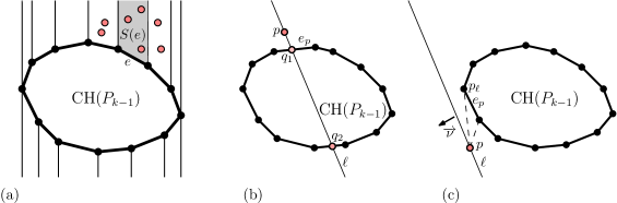
Figure 1: (a) The conflict list $C_{e}$ of the edge $e\in E(P_{k-1})$ contains all the lightly-shaded points, whereas the refined conflict list $C^{*}(e)$ has only those points in the vertical slab $S(e)$; (b–c) The edge $e_{p}$ of $E(P_{k-1})$ is visible to $p$ when (b) $\ell$ intersects $\operatorname{CH}(P_{k-1})$, or (c) $\ell$ does not meet $\operatorname{CH}(P_{k-1})$. In this case $p_{\ell}$ is an extreme vertex for the direction $\overrightarrow{\nu}$, and the two dashed lines depict the visibility lines between $p$ and the two respective endpoints of $e_{p}$.

We next process the lines in $L_{2}$. Note that all points on the lines in $L_{2}$ conflict with at least one edge in $E(P_{k-1})$, since no line in $L_{2}$ meets $\operatorname{CH}(P_{k-1})$. To find these edges we determine for each $\ell\in L_{2}$ a vertex $p_{\ell}$ on the boundary of $\operatorname{CH}(P_{k-1})$ that is extreme for $\ell$. This can be done in total time $O(n)$ by ordering $E(P_{k-1})$ and $L_{2}$ according to their slopes (the latter being performed during preprocessing), and then merging these two lists in linear time. Next, fix such a line $\ell\in L_{2}$, and let $p\in\ell$ be a query point, then $p$ must see one of the two edges in $E(P_{k-1})$ incident to $p_{\ell}$ (which can be determined in constant time given $p_{\ell}$), and we thus set $e_{p}$ to be the corresponding edge; see Figure 1(c).

We are now ready to determine, for each point $p\in P_{k}$ outside $\operatorname{CH}(P_{k-1})$, the slab $S(e_{p}^{*})$ that contains it (note that $e_{p}^{*}$ must be vertically visible from $p$). If $e_{p}$ is vertically visible from $p$, we set $e_{p}^{*}:=e_{p}$. Otherwise, we walk along (the boundary of) $\operatorname{CH}(P_{k-1})$, starting from $e_{p}$ and progressing in the appropriate direction (uniquely determined by $p$ and $e_{p}$), until the slab containing $p$ is found. Using cross pointers between the edges and the points, we can easily compute $C^{*}_{e}$ for each $e\in E(P_{k-1})$. By construction, all traversed edges are in conflict with $p$, and thus the overall time for this procedure is proportional to the total size of the conflict lists $C_{e}$. Recalling that $c_{e}=|C_{e}|$, we obtain

$$\operatorname{\mathbf{Exp}}\Bigl{[}\sum_{e\in E(P_{k-1})}c_{e}\Bigr{]}=O(z_{k})=O(n),$$

by Lemma 2.1 with $f:m\mapsto m$. This concludes the construction of the refined conflict lists.

Computing $\operatorname{CH}(P_{k})$. We next describe how to construct the upper hull of $P_{k}$, the analysis for the lower hull is analogous. Let $\langle e_{1},\ldots,e_{s}\rangle$ be the edges along the upper hull of $P_{k-1}$, ordered from left to right. For each $e_{i}$, we sort the points in $C^{*}_{e_{i}}$ according to their $x$-order, using, e.g., merge sort. We apply the same procedure for the extreme points. We then concatenate the sorted lists $C^{*}_{v_{l}},C^{*}_{e_{1}},C^{*}_{e_{2}},\ldots,C^{*}_{e_{s}},C^{*}_{v_{r}}$, and merge the result with the vertices of the upper hull of $P_{k-1}$. Call the resulting list $Q$, and use Graham’s scan to find the upper hull of $Q$ in time $O(|Q|)$. This is also the upper hull of $P_{k}$. Applying once again Lemma 2.1 with $f:m\mapsto m\log m$, and putting $c^{*}_{e}:=|C^{*}_{e}|$, $c^{*}_{v_{l}}:=|C^{*}_{v_{l}}|$, $c^{*}_{v_{r}}:=|C^{*}_{v_{r}}|$, and $A>0$ an absolute constant, the overall expected running time of this step is bounded by

$$\operatorname{\mathbf{Exp}}\bigl{[}A\cdot(c^{*}_{v_{l}}\log{c^{*}_{v_{l}}}+c^{*}_{v_{r}}\log{c^{*}_{v_{r}}}+\sum_{e\in E(P_{k-1})}c^{*}_{e}\log c^{*}_{e})\bigr{]}$$

$$\leq\operatorname{\mathbf{Exp}}\bigl{[}3A\cdot\sum_{e\in E(P_{k-1})}c_{e}\log c_{e}\bigr{]}=O\left(z_{k}\log\left(z_{k}/z_{k-1}\right)\right)$$

$$=O\left((n/\log^{(k)}n)\log\left(\log^{(k-1)}n/\log^{(k)}n\right)\right)=O(n),$$

because by definition $C^{*}_{e}\subseteq C_{e}$, so $c^{*}_{e}\leq c_{e}$, and $c^{*}_{v_{l}}\leq c_{e_{1}}+c_{e_{2}}$ for two edges $e_{1}$, $e_{2}$ of $E(P_{k-1})$ (and similarly for $c^{*}_{v_{r}}$). In total, we obtain that the expected time to construct $\operatorname{CH}(P_{k})$ given $\operatorname{CH}(P_{k-1})$ is $O(n\alpha(n))$, and since there are $\log^{*}n$ iterations, the total running time is $O(n\alpha(n)\log^{*}n)$.

We note that the analysis proceeds almost verbatim when $L$ is just a set of line segments in the plane. In this case, we preprocess the lines containing the input segments, and proceed as in the original problem. We have thus shown:

Theorem 2.2.

Using $O(n^{2})$ space and time, we can preprocess a set $L$ of $n$ lines in the plane (given in general position), such that given any point set $P$ with each point lying on a distinct line in $L$, we can construct $\operatorname{CH}(P)$ in expected time $O(n\alpha(n)\log^{*}n)$. The same result holds if $L$ is a set of $n$ line segments whose supporting lines are in general position.

Remark. An inspection of the proof of Theorem 2.2 shows that the total expected conflict size, over all iterations $k$, is only $O(n)$.

2.2 Better Bounds for Oblivious Points

We now present an improved solution under the obliviousness model, where we assume that the points are oblivious to the random choices during the preprocessing step. Specifically, this implies that an adversary cannot pick the point set $P$ in a malicious manner, as it is not aware of the random choices at the preprocessing step. This fairly standard assumption has appeared in various studies (see, e.g., [1, 11]). In the discussion at the end of this section we describe this issue in more detail.

Preprocessing. We now construct a gradation $L_{1}\subseteq L_{2}\subseteq\cdots\subseteq L_{1+\log\log n}=L$ of the lines during the preprocessing phase, where the set sizes decrease geometrically. Specifically, $|L_{1}|=y_{1}=\lceil n/\log{n}\rceil$, and for $k=2,\ldots,1+\log\log{n}$, $L_{k-1}$ is a random subset of $L_{k}$ of size

$$|L_{k-1}|=y_{k-1}:=\left\lceil{\frac{y_{k}}{2}}\right\rceil=\left\lceil{\frac{1}{2}\cdot\frac{n}{2^{\log\log{n}-k+1}}}\right\rceil.$$ (1)

We construct each arrangement ${\mathcal{A}}(L_{k})$ in $O(n^{2}2^{2k-2}/\log^{2}{n})$ time, for a total $O(n^{2})$ time over all gradation steps.

Query. Given an exact input $P$, we first follow the gradation produced at the preprocessing stage, and generate the corresponding gradation $P_{1}\subseteq P_{2}\subseteq\ldots\subseteq P_{1+\log\log{n}}=P$, where $P_{k}=P\cap L_{k}$, for all $k$. By the obliviousness assumption, each $P_{k-1}$ is an unbiased sample of $P_{k}$, so Lemma 2.1 applies (see once again the discussion below). Moreover, the key observation is that in order to obtain $\operatorname{CH}(P_{k})$ from $\operatorname{CH}(P_{k-1})$, it suffices to confine the search to the arrangement ${\mathcal{A}}(L_{k})$ instead of the entire arrangement ${\mathcal{A}}(L)$ as in Section 2.1. Thus, we first construct $\operatorname{CH}(P_{1})$ in $O(n)$ time as before. Next, to obtain $\operatorname{CH}(P_{k})$ from $\operatorname{CH}(P_{k-1})$, we construct the zones of $\operatorname{UH}(P_{k-1})$ and $\operatorname{LH}(P_{k-1})$ in ${\mathcal{A}}(L_{k})$ in $O(y_{k}\alpha(y_{k}))$ time, and then compute the refined conflict lists just as in Section 2.1. The overall expected time to produce these lists is $O(y_{k})$, totaling $O(n)$ over all steps. As in Section 2.1, the expected time (of the final step) to compute $\operatorname{UH}(P_{k})$ and $\operatorname{LH}(P_{k})$ is $O\left(y_{k}\log\left(y_{k}/y_{k-1}\right)\right)=O\left(y_{k}\right)$,

by (1). Thus, the expected running time at the $k$th step is dominated by the zone construction, so the overall expected running time is

$O\left(\sum_{k=1}^{1+\log\log{n}}y_{k}\alpha(y_{k})\right)=O\left(n\alpha(n)\right)$, as is easily verified. Thus,

Theorem 2.3.

Using $O(n^{2})$ space and time, we can preprocess a set $L$ of $n$ lines in the plane, such that for any point set $P$ with each point lying on a distinct line of $L$, we can construct $\operatorname{CH}(P)$ in expected time $O(n\alpha(n))$ assuming obliviousness.

Discussion. The issue captured by the obliviousness assumption is: how much does the adversary know about the preprocessing phase? If the adversary manages to obtain the coin flips performed during the preprocessing stage, then this enables a malicious choice of the input. This phenomenon is particularly striking in the case of hashing: if the adversary knows the random choice of the hash function, a bad set of inputs can hash all keys to a single slot, completely destroying the hash table. On the other hand, if the adversary is oblivious to the hash function, the expected running time per operation is only $O(1)$; see, e.g., [18, Chapter 11].

In our model we encounter a similar phenomenon. Even though the impact is not as disastrous as for hashing, assuming obliviousness for the adversary can improve our running time by a factor of $O(\log^{*}n)$. To illustrate the effect of obliviousness in our setting, consider the scenario illustrated in Figure 2. In this case, we have a set $L$ of lines and a random subset $L^{\prime}\subseteq L$. The adversary can pick the point set $P$ so that $P^{\prime}:=P\cap L^{\prime}$ is a biased sample of $P$ in a sense that violates the properties of Lemma 2.1. In particular, the total number of conflicts between the edges of $\operatorname{CH}(P^{\prime})$ and $P$ may become quadratic, which makes the random incremental construction inefficient. Nevertheless, if the adversary is oblivious with respect to the sample, the points in $P^{\prime}$ behave as an unbiased sample of $P$.

Figure 2: Illustrating the obliviousness assumption. The set $L$ contains all the lines in the figure. The set $L^{\prime}$ of the dashed lines depicted in the figure is a random subset of $L$. If the adversary knows this random subset $L^{\prime}$, it can place the points $p_{1},\ldots,p_{8}$ as illustrated in the figure, thereby constructing $\operatorname{CH}(p_{1},\ldots,p_{4})$ first. Then each edge on the upper hull $\operatorname{UH}(p_{1},\ldots,p_{4})$ is in conflict with each of the remaining points $p_{5},\ldots,p_{8}$.

2.3 Extensions and Variants

Diameter- and width-queries. Given $\operatorname{CH}(P)$, we can easily compute the diameter (i.e., a pair of points with maximum Euclidean distance) and the width of $P$ (a strip of minimal width containing all the points in $P$) in linear time (see, e.g., [37, Chapter 4]). Hence,

Corollary 2.4.

Using $O(n^{2})$ space and time, we can preprocess a set $L$ of $n$ lines in the plane, such that given a point set $P$ with each point lying on a distinct line of $L$, the diameter or width of $P$ can be found in expected time $O(n\alpha(n)\log^{*}n)$. The expected running time becomes $O(n\alpha(n))$ assuming obliviousness.

A trade-off between space and query time. Our data structure can be generalized to support a trade-off between preprocessing time (and storage) and the query time, using a relatively standard grouping technique [2, 9], described as follows.

Preprocessing. Let $1\leq m\leq n$ be a parameter, and, without loss of generality, assume that $n/m$ is an integer. We partition $L$ into $m$ subsets $L_{1},\ldots,L_{m}$ of size $n/m$ each, and construct the arrangements ${\mathcal{A}}(L_{k})$, for $k=1,\ldots,m$, in overall time and storage $O(n^{2}/m)$ (cf. [2, 9]).

Query. Given an exact input $P$, we first construct $\operatorname{CH}(P_{k})$, where $P_{k}$ is the subset of points on the lines in $L_{k}$, $k=1,\ldots,m$, in $O((n/m)\alpha(n/m)\log^{*}{(n/m)})$ (assuming obliviousness it is $O((n/m)\alpha(n/m))$) expected time, for a total expected time of $O(n\alpha(n/m)\log^{*}{(n/m)})$ (resp., $O(n\alpha(n/m))$) over all these subsets. Having $\operatorname{CH}(P_{k})$ at hand for all $k$, we merge $\operatorname{UH}(P_{1})$, $\ldots$, $\operatorname{UH}(P_{m})$ in $O(n\log{m})$ time [18], thereby producing a list $Q$ of points sorted according to their $x$-order. We then use Graham’s scheme to construct the upper hull of $Q$ (and thus of $P$) in $O(|Q|)$ time. We produce the lower hull of $P$ in an analogous manner. We have thus shown:

Corollary 2.5.

Fix $1\leq m\leq n$. In total $O(n^{2}/m)$ time and space, we can preprocess a set $L$ of $n$ lines in the plane, such that given a point set $P$ with each point lying on a distinct line of $L$, we can construct $\operatorname{CH}(P)$ in expected time $O(n(\log{m}+\alpha(n/m)\log^{*}{(n/m)}))$. The running time becomes $O(n(\log{m}+\alpha(n/m)))$ assuming obliviousness.

Note that for small values of $m$, Corollary 2.5 in fact yields an improvement over Theorem 2.2. Specifically, by setting $m:=2^{\alpha(n)}$, we have that the space and preprocessing requirement in Theorem 2.2 can be lowered to $O(n^{2}/2^{\alpha(n)})$, while the expected query time remains $O(n\alpha(n)\log^{*}(n))$.

Discussion. As noted in the introduction, the bounds in Corollary 2.5 are somewhat disappointing. However, the study by Ali Abam and de Berg [2] might provide (albeit, weak) evidence that these bounds are unlikely to be improved. Indeed, they have studied the kinetic sorting problem, where we are given a set of $n$ points moving continuously on the real line, and the goal is to maintain a structure on them so that at any given time the points can be sorted efficiently. Ali Abam and de Berg [2] showed that even when the trajectories of these points are just linear functions, then under the comparison graph model (see [2] for the definition) one cannot answer a query faster than $cn\log{m}$ time using less than $c^{\prime}n^{2}/m$ preprocessing time and storage, for appropriate absolute constants $c,c^{\prime}>0$. As discussed in [2], this may indicate that better trade-offs for the kinetic convex hull problem seem unlikely. Nevertheless, it may not provide a rigorous proof, as the analysis for the kinetic sorting problem strongly relies on the one-dimensionality of the points, and does not work for points in the plane, at least under the context of the proofs given in [2]. Still, we have chosen to present those details in this paper, as we tend to believe that bounds of this kind could also apply to our problem (which is even more difficult than the kinetic convex hull problem, as described in the introduction), and that a rigorous analysis could stem from the approach in [2]. This would imply that the trade-off bounds given in Corollary 2.5 are nearly optimal.

An output-sensitive algorithm. Our algorithm can be made sensitive to the size $h$ of the convex hull by adapting a technique of Ali Abam and de Berg [2] that uses gift wrapping queries. The setting for queries of this kind is as follows. Let $Q$ be a point set, given an arbitrary point $p$ (not necessarily from $Q$) and a line $\ell$ through $p$, such that all points of $Q$ lie on the same side of $\ell$, report a point $q\in Q$ that is hit first when $\ell$ is rotated around $p$ (say, in clockwise direction).

A search on the value of $h$. Since the output size $h$ is not given in advance, we perform a search on its actual value, over at most $\log^{*}{n}-1$ iterations, in the query step, and apply all tested values at the preprocessing step, as described below. The tested values of $h$ are chosen in the following manner. Let $h_{i}$ be the value of $h$ at the $i$th round. Initially, $h_{1}=1$, and put $h_{i}=2^{(i-1)}$, for $i\geq 2$, where $2^{(\cdot)}$ is the power-tower function. We continue the search as long as $h_{i}\leq\log{n}$; let $t$ be the number of rounds thus obtained. By construction $t\leq\log^{*}{n}-1$. When $h_{i}>\log{n}$, we stop the search and resort to the bound in Theorem 2.2—see below.

Preprocessing. At each round $i=1,\ldots,t$, we set a parameter $m_{i}$ to be

$$m_{i}:=\max\left\{1,\frac{n}{h_{i}\log{h_{i}}}\right\},$$

and partition $L$ into $m_{i}$ roughly equal subsets $L^{(i)}_{1},\ldots,L^{(i)}_{m_{i}}$. We then proceed in a similar manner as described earlier for the trade-off between space and query time. That is, for each $k=1,\ldots,m_{i}$, we construct the arrangement ${\mathcal{A}}(L^{(i)}_{k})$ in overall time and storage $O(n^{2}/m_{i})$.

The total time and storage consumed over all rounds $i$ is thus

$$O\left(n^{2}+\sum_{i=1}^{t}nh_{i}\log{h_{i}}\right)=O(n^{2}),$$

since the sum over the rounds $i$ is dominated by the last term, which is $O(n\log{n}\log\log{n})$.

Query. Given a point set $P$ with each point lying on a distinct line of $L$, we construct $\operatorname{CH}(P)$ in an output-sensitive manner, as follows.

At the $i$th round, let $P^{(i)}_{k}:=P\cap L^{(i)}_{k}$, for $k=1,\ldots,m_{i}$. Construct $\operatorname{CH}(P^{(i)}_{1})$, $\operatorname{CH}(P^{(i)}_{2})$, $\ldots$, $\operatorname{CH}(P^{(i)}_{m_{i}})$, as in Section 2.1. This takes total time $O(n\alpha(n/m_{i})\log^{*}{(n/m_{i})})=O(n\alpha(h_{i})\log^{*}(h_{i}))$ (resp. $O(n\alpha(n/m_{i}))=O(n\alpha(h_{i}))$ assuming obliviousness).

The primitive operation we would like to obtain is a gift wrapping query on $P$. To this end, we perform standard gift wrapping queries for each subset $P^{(i)}_{k}$ in $O(\log{(n/m_{i})})$ time (see, e.g., [37]). This yields a set of $m_{i}$ candidates, from which we produce the final answer to the query. In total, a gift wrapping query takes $O(m_{i}\log{(n/m_{i})})=O(n/h_{i})$ steps.

We now attempt to construct $\operatorname{CH}(P)$. We begin with a gift wrapping query for the leftmost vertex $p$ of $P$ and the vertical line $\ell_{p}$ passing through $p$. This yields a pair $(p^{\prime},\ell^{\prime})$, where $p^{\prime}$ is the first point hit by $\ell$, and $\ell^{\prime}$ is the line through $p$ and $p^{\prime}$. We continue until (i) we hit $p$ again, or (ii) we have performed $h_{i}$ gift wrapping queries. This results in a running time of

$$O\left(h_{i}\cdot m_{i}\log{(n/m_{i})}\right)=O\left(h_{i}\cdot\frac{n}{h_{i}}\right)=O(n).$$

The round succeeds if we reach $p$. Otherwise it fails, and we proceed to round $i+1$. After $t\leq\log^{*}n-1$ unsuccessful rounds (i.e., if $h_{i}>\log{n}$), we compute $\operatorname{CH}(P)$ directly via Theorem 2.2.

It is easy to verify that the actual number of rounds that we need is at most $O(\log^{*}h)$. Combining the bounds above, it follows that the overall query time is $O(n\alpha(h)(\log^{*}{h})^{2})$ (or $O(n\alpha(h)\log^{*}{h})$ assuming obliviousness), as asserted. We have thus shown:

Corollary 2.6.

In total $O(n^{2})$ time and space, we can preprocess a set $L$ of $n$ lines in the plane, such that given a point set $P$ with each point lying on a distinct line of $L$, $\operatorname{CH}(P)$ can be found in expected time $O(n\alpha(h)(\log^{*}{h})^{2})$, where $h$ is the output size. The expected running time becomes $O(n\alpha(h)\log^{*}h)$ assuming obliviousness.

3 Levels in Arrangements

Preliminaries. Let $L$ be a set of $n$ lines in the plane (in general position). Given a point $p$, the level of $p$ with respect to $L$ is the number of lines in $L$ intersected by the open downward vertical ray emanating from $p$. For an integer $k\geq 0$, the $k$-level of the arrangement ${\mathcal{A}}(L)$, denoted by $\operatorname{lev}_{k}(L)$, is the closure of all edges of ${\mathcal{A}}(L)$ whose interior points have level $k$ with respect to $L$. It is a monotone piecewise-linear chain. In particular, $\operatorname{lev}_{0}(L)$ is the so-called “lower envelope” of $L$; see, e.g., [41, Chapter 5.4] and Figure 3. The $(\leq k)$-level of ${\mathcal{A}}(L)$, denoted by $\operatorname{lev}_{\leq k}(L)$, is the complex induced by all cells of ${\mathcal{A}}(L)$ lying on or below the $k$-level, and thus its edge set is the union of $\operatorname{lev}_{i}(L)$ for $i=0,\ldots,k$; its overall combinatorial complexity is $O(nk)$ (see, e.g., [16, 41]).

In what follows we denote by $V_{q}(M)$ (resp., $V_{\leq q}(M)$) the set of vertices of $\operatorname{lev}_{q}(M)$ (resp., $\operatorname{lev}_{\leq q}(M)$), where $q\geq 0$ is an integer parameter and $M$ is a set of lines in the plane. It is easy to verify that the combinatorial complexity of $\operatorname{lev}_{q}(M)$ is at most $O(1+|V_{q}(M)|)$ (see once again [41]). Throughout this section, we use the Vinogradov-notation: $f\ll g$ means $f=O(g)$ and $f\gg g$ means $f=\Omega(g)$. In addition, we write $\operatorname{\mathbf{Exp}}_{X}[\cdot]$ to emphasize that we take the expectation with respect to the random choice of $X$ (the other variables are considered constant).

Figure 3: The $2$-level in an arrangement of lines.

The best currently known bound for the worst-case complexity of $\operatorname{lev}_{k}(L)$ is $O(nk^{1/3})$ [21]. Nevertheless, since the overall combinatorial complexity of, say, $\operatorname{lev}_{\leq 2k}(L)$ is only $O(nk)$ [16], it follows that the average size of $V_{i}(L)$, for each $i=k,\ldots,2k$, is only $O(n)$. Specifically, we have (see also [23] for a similar property):

Claim 3.1.

Let $\tilde{k}$ be a random integer in the range $\{k$, $\ldots$, $2k\}$. Then, for any subset $S\subseteq L$, we have

$$\operatorname{\mathbf{Exp}}_{\tilde{k}}[|V_{\tilde{k}}(S)|]\ll|S|.$$

Proof.

The claim follows from the observation that the total size of $V_{\leq 2k}(S)$ is $O(|S|k)$, and each vertex appears in exactly two consecutive levels of ${\mathcal{A}}(S)$. ∎

The problem. In the sequel we study the following problem. We are given a set $P=\{p_{1},\ldots,p_{n}\}$ of $n$ points in the plane (in general position), and we would like to compute a data structure such that, given any set $L=\{\ell_{1},\ldots,\ell_{n}\}$ of $n$ lines satisfying $p_{i}\in\ell_{i}$, for $i=1,\ldots,n$, and any parameter $k\geq 0$, we can efficiently construct $\operatorname{lev}_{\leq k}(L)$. This is a natural generalization of the problem studied in Section 2.1. Indeed, let us apply the standard duality transformation, where a line $l:\;y=ax+b$ is mapped to the point $l^{*}=(a,-b)$, and a point $p=(c,d)$ is mapped to the line $p^{*}:\;y=cx-d$ (see, e.g., [6, Chapter 8]). Then $\operatorname{lev}_{0}(L)$ in the “primal” plane is mapped to the (upper) convex hull of the points $L^{*}$ in the “dual” plane. Everett et al. [23] showed that $\operatorname{lev}_{\leq k}(L)$ can be constructed in $O(n\log n+nk)$ time, and that this time bound is worst-case optimal (see also [10]). We show:

Theorem 3.2.

Using $O(n^{2})$ space and time, we can preprocess a set $P$ of $n$ points in the plane, such that given a set $L$ of lines with each line incident to a distinct point of $P$, $\operatorname{lev}_{\leq k}(L)$ can be computed in expected time $O(n\alpha(n)(\log^{*}n-\log^{*}k)+nk)$. The expected running time becomes $O(n\alpha(n)+nk)$ assuming obliviousness.

Theorem 3.2 improves the “standard” bound of $O(n\log n+nk)$ for any $k=o(\log{n})$. We combine ideas from Chan’s algorithm for constructing $(\leq k)$-levels in arrangements of planes in ${\mathbb{R}}^{3}$ [10] with the technique of Everett et al. [23]. The preprocessing phase is fairly simple, but the details of the query processing and its analysis are more intricate. We begin with an overview of the approach, and then describe the query step and its analysis in more detail.

An overview of the algorithm. The main ingredients of the algorithm are as follows.

Preprocessing. Compute the arrangement ${\mathcal{A}}(P^{*})$ of the lines dual to the points in $P$ (and produce its vertical decomposition) in $O(n^{2})$ time and storage.

Query. We are given a set of lines $L$ as above, and an integer $k\geq 0$. If $k\geq\log{n}$ we use the algorithm of Everett et al. [23] to report $\operatorname{lev}_{\leq k}(L)$ in $O(n\log n+nk)=O(nk)$ time. Otherwise, we compute a gradation $L_{1}\subseteq L_{2}\subseteq\cdots\subseteq L_{\log^{*}n-\log^{*}k+1}\subseteq L$ of $L$. The sizes of the subsets $L_{i}$ are similar to those presented in Section 2.1 for the dual plane, but as soon as the number of lines in a subset of the gradation exceeds $\lceil{n/k}\rceil$, we complete the sequence in a single step by choosing the next subset to be the entire set $L$. As in Section 2.1, we set $|L_{1}|:=\lceil{n/\log n}\rceil$.

We choose a random integer $\tilde{k}\in\{k,\ldots,2k\}$. Then, at the first iteration, we construct $\operatorname{lev}_{\leq\tilde{k}}(L_{1})$ in $O(nk)$ time, using the algorithm in [23]. At each of the following iterations $i$, we construct $\operatorname{lev}_{\leq\tilde{k}}(L_{i})$ from $\operatorname{lev}_{\leq\tilde{k}}(L_{i-1})$ (at the final step, we construct $\operatorname{lev}_{\leq\tilde{k}}(L)$ from $\operatorname{lev}_{\leq\tilde{k}}(L_{\log^{*}n-\log^{*}k+1})$). As observed above, the random choice of $\tilde{k}$ guarantees that the expected complexity of each $\operatorname{lev}_{\tilde{k}}(L_{i})$ is only linear in $|L_{i}|$, for each $i=2,\ldots,\log^{*}n-\log^{*}k+1$, which is crucial for the analysis. Finally, we eliminate from $\operatorname{lev}_{\leq\tilde{k}}(L)$ all portions lying above the (actual) $k$-level, in order to obtain the final structure $\operatorname{lev}_{\leq k}(L)$.

To construct $\operatorname{lev}_{\leq\tilde{k}}(L_{i})$ from $\operatorname{lev}_{\leq\tilde{k}}(L_{i-1})$, we would like to proceed as follows. We compute $\operatorname{UH}(\operatorname{lev}_{\leq\tilde{k}}(L_{i-1}))$ and subdivide it into semi-unbounded (in the negative $y$-direction) trapezoidal cells. The first goal is to find for each such cell $\Delta$ the set of lines $C_{\Delta}\subseteq L_{i}$ which are in conflict with $\Delta$ (that is, $\Delta\cap\ell\neq\emptyset$, for each $\ell\in C_{\Delta}$). This goal is achieved by mapping $\operatorname{UH}(\operatorname{lev}_{\leq\tilde{k}}(L_{i-1}))$ to the dual plane and walking along its zone in ${\mathcal{A}}(P^{*})$. The dual of $\operatorname{UH}(\operatorname{lev}_{\leq\tilde{k}}(S))$ is a concave chain $\gamma$ (the lower envelope of the lines dual to the vertices of $\operatorname{UH}(\operatorname{lev}_{\leq\tilde{k}}(S))$), where each vertex $v$ of $\operatorname{UH}(\operatorname{lev}_{\leq\tilde{k}}(S))$ is mapped to an edge $v^{*}$ of $\gamma$ and each edge $e$ is mapped to a vertex $e^{*}$ of $\gamma$. Moreover, a line $\ell\in L$ below a vertex $v$ of $\operatorname{UH}(\operatorname{lev}_{\leq\tilde{k}}(S))$ is mapped to a point $\ell^{*}$ (on some line of $P^{*}$) above the corresponding edge $v^{*}$ of $\gamma$. As is easily verified, such a line $\ell$ intersects $\operatorname{UH}(\operatorname{lev}_{\leq\tilde{k}}(S))$. Otherwise, if $\ell$ lies above all the vertices of $\operatorname{UH}(\operatorname{lev}_{\leq\tilde{k}}(S))$, then $\ell\cap\operatorname{UH}(\operatorname{lev}_{\leq\tilde{k}}(S))=\emptyset$, and this implies that $\ell^{*}$ lies below $\gamma$ in the dual plane. See Figure 4(a)–(b).

Having the lists $C_{\Delta}$ at hand, we construct for each $\Delta$ the structure $\operatorname{lev}_{\leq\tilde{k}}(L_{i})$ clipped to $\Delta$ by (i) constructing $\operatorname{lev}_{\tilde{k}}(C_{\Delta})$ (clipped to $\Delta$); (ii) clipping each line $\ell\in C_{\Delta}$ to its portion that lies below $\operatorname{UH}(\operatorname{lev}_{\tilde{k}}(C_{\Delta})\cap\Delta)$; (iii) constructing the arrangement of these portions within $\Delta$ (as observed in [23], the actual level of these portions in ${\mathcal{A}}(L_{i})$ does not exceed $2\tilde{k}-1$); and (iv) eliminating from the arrangement just computed all portions lying above $\operatorname{lev}_{\tilde{k}}(C_{\Delta})\cap\Delta$. Finally, we glue the resulting structures together and report $\operatorname{lev}_{\leq\tilde{k}}(L_{i})$.

However, it would be too expensive to process each conflict list $C_{\Delta}$ individually. Therefore, a crucial ingredient of the algorithm is to consider blocks instead of just individual cells. Specifically, we gather contiguous cells into blocks and process them all together. This partition is the key to reducing the number of cells considered in the update step; see Figure 5. The bulk of the analysis lies in a careful balancing between the block sizes and their overall number, and in particular showing that blocks with large conflict lists are scarce.

3.1 Query Processing

We now describe the query process and its analysis in more detail. We first follow a gradation as described in the overview, and then proceed to the update step.

The update step. From now on we fix an iteration $i>1$, and, with a slight abuse of notation, put $S:=L_{i-1}$ and $L:=L_{i}$. Let $p:=|S|/|L|$. By definition, $S$ is a random sample of $L$ of size $\lceil{n/\log^{(i-1)}n}\rceil=p|L|$. Given $\operatorname{lev}_{\leq\tilde{k}}(S)$, we first construct $\operatorname{UH}(\operatorname{lev}_{\leq\tilde{k}}(S))$.

Claim 3.3.

The overall expected time to construct $\operatorname{UH}(\operatorname{lev}_{\leq\tilde{k}}(S))$ is $O(|S|)$.

Proof.

Using easy manipulations on the DCEL representing $\operatorname{lev}_{\leq\tilde{k}}(S)$, we can first locate a vertex $v$ of $\operatorname{lev}_{\tilde{k}}(S)$, and then proceed to its neighboring topmost vertex (say, to its left) by walking along its corresponding adjacent edge. We then continue progressing in this manner to the left. The vertices to the right of $v$ are explored analogously. Thus we can extract the sequence of vertices (and edges) along $\operatorname{lev}_{\tilde{k}}(S)$, ordered from left to right. By Claim 3.1, its expected size is $O(|S|)$. Then we use Graham’s scan on the resulting set of vertices. ∎

Next, we shoot vertical rays from each vertex of the hull $\operatorname{UH}(\operatorname{lev}_{\leq\tilde{k}}(S))$ in the negative $y$-direction. This gives a collection ${\mathcal{T}}_{\tilde{k},S}$ of semi-unbounded trapezoidal cells covering $\operatorname{UH}(\operatorname{lev}_{\leq\tilde{k}}(S))$, and hence also $\operatorname{lev}_{\leq\tilde{k}}(L)$, as is easily verified (see, e.g., [35] for similar arguments). We group the cells in ${\mathcal{T}}_{\tilde{k},S}$ into $O(|{\mathcal{T}}_{\tilde{k},S}|(p/\tilde{k}))$ semi-unbounded vertical strips, each of which consists of $\tilde{k}/p$ contiguous cells. Such a vertical strip is called a block. Every block is bounded by a convex chain from above, and by two vertical walls, one to its left and the other to its right. Let $\mathcal{B}$ be the set of all blocks.

We say that a line $\ell\in L$ is in conflict with a cell $\Delta\in{\mathcal{T}}_{\tilde{k},S}$, if $\Delta\cap\ell\neq\emptyset$. The conflict list $C_{\Delta}$ is then the set of all lines $\ell\in L$ in conflict with $\Delta$, and we put $c_{\Delta}:=|C_{\Delta}|$. We similarly define conflict lists $C_{B}$ and conflict sizes $c_{B}$ for each block $B\in\mathcal{B}$. Our next goal is to determine the conflict lists $C_{B}$ for each block.

Lemma 3.4.

We can construct the conflict lists $C_{B}$, $B\in\mathcal{B}$, in overall time

$$O\left(n\alpha(n)+|V_{\tilde{k}}(S)|+\sum_{B\in\mathcal{B}}c_{B}\right).$$

Proof.

First, we determine for each line $\ell\in L$ one trapezoid $\Delta_{\ell}\in{\mathcal{T}}_{\tilde{k},S}$ such that $\ell\in C_{\Delta_{\ell}}$, if such a $\Delta_{\ell}$ exists. This is done by a walk in the dual plane, as described in the overview above and illustrated in Figure 4. Specifically, we dualize $\operatorname{UH}(\operatorname{lev}_{\leq\tilde{k}}(S))$ to a concave chain $\gamma$.

Figure 4: (a) The $\tilde{k}$-level of ${\mathcal{A}}(S)$ is depicted by the lightly-shaded polygonal line in the figure, and $\operatorname{UH}(\operatorname{lev}_{\leq\tilde{k}}(S))$ is depicted by the dashed line. The line $\ell^{\prime}$ passes above $\operatorname{UH}(\operatorname{lev}_{\leq\tilde{k}}(S))$, where $\ell$ passes below $v$ and thus meets $\operatorname{UH}(\operatorname{lev}_{\leq\tilde{k}}(S))$. (b) The dual scene of (a). The concave chain $\gamma$ is the dual of $\operatorname{UH}(\operatorname{lev}_{\leq\tilde{k}}(S))$. The line $\ell$ is mapped to the point $\ell^{*}$, where the pair of the dashed lines depict the visibility lines of $\ell^{*}$ to $\gamma$. The line $\ell^{\prime}$ is mapped to the point $\ell^{\prime*}$ lying below $\gamma$.

Using a similar technique as in Section 2.1, we walk along the zone of $\gamma$ in ${\mathcal{A}}(P^{*})$ in order to determine, for each point $\ell^{*}$ corresponding to a line $\ell\in L$, its orientation with respect to $\gamma$. When $\ell^{*}$ lies above $\gamma$, we find an edge $v^{*}_{\ell^{*}}$ of $\gamma$ that is visible from $\ell^{*}$. Using the corresponding vertex $v_{\ell}$ in the primal plane, we can determine a cell $\Delta_{\ell}$ that is intersected by $\ell$.

Next, we determine for each such line $\ell$ a block $B$ that conflicts with it, namely the block that contains $\Delta_{\ell}$. We then find all blocks $B^{\prime}$ with $\ell\in C_{B^{\prime}}$ through a bidirectional walk from $B$. That is, we can determine if $\ell$ intersects the next block by checking whether $\ell$ intersects any of its walls (otherwise, $\ell$ intersects its convex chain). See Figure 5.

The bound on the running time now follows using similar considerations as in Section 2.1. ∎

Figure 5: The block $B$ is depicted by the lightly-shaded region. The line $\ell_{1}$ does not intersect any neighboring block, whereas $\ell_{3}$ and $\ell_{4}$ also meet the left neighbor of $B$. The line $\ell_{2}$ meets both neighbors.

Our next goal is to determine the $(\leq\tilde{k})$-level clipped to $B$, for each $B\in\mathcal{B}$. To this end, we use a variant of the technique of Everett et al. [23].

Lemma 3.5.

Let $B\in\mathcal{B}$. The $(\leq\tilde{k})$-level of $L$ clipped to $B$ can be constructed in time $O(c_{B}\log{c_{B}}+(m_{B}+c_{B})\log^{2}k+a_{B})$, where $c_{B}:=|C_{B}|$, $m_{B}:=|V_{\tilde{k}}(C_{B})\cap B|$, and $a_{B}$ is the number of vertices of ${\mathcal{A}}(L)$ below $\operatorname{UH}(\operatorname{lev}_{\tilde{k}}(C_{R})\cap B)$.

Proof.

We apply the algorithm of Cole et al. [17] in order to construct $\operatorname{lev}_{\tilde{k}}(C_{B})\cap B$ in time $O(c_{B}\log{c_{B}}+(m_{B}+c_{B})\log^{2}\tilde{k})$. Note that this algorithm returns $\operatorname{lev}_{\tilde{k}}(C_{B})\cap B$ as an $x$-monotone polygonal chain $\zeta$ ordered from left to right. Next, we determine for each line $\ell\in C_{B}$ its first and last intersections $w_{1}$, $w_{2}$ with $\zeta$ (if they exist). Clearly, the portion of $\ell$ below $\operatorname{UH}(\zeta)$ is either (i) the line segment $w_{1}w_{2}$ (if both intersections exist); (ii) a ray with an endpoint at $w_{1}$ (if $w_{1}$ is the only intersection with $\operatorname{UH}(\zeta)$) or (iii) the full line $\ell$ clipped to $B$ (if it lies fully below $\zeta$).

These intersections can easily be determined in $O(m_{B})$ time by walking along $\zeta$ and recording for each line $\ell$ the first and last vertices of $\zeta$ that are incident to $\ell$ (if they exist); at the representation of $\zeta$, we also store the incident lines within each vertex. A line that is not encountered during this process, does not meet $\zeta$, and we can easily check whether it lies below $\zeta$. As observed above, each of these portions (clipped to $B$) is either the (full) line $\ell$, a ray, or a line segment. Let $C_{B}^{\prime}$ be the resulting set of these portions; by construction, $c_{B}^{\prime}:=|C_{B}^{\prime}|\leq c_{B}$. Having this collection at hand, the computation of $\operatorname{lev}_{\leq\tilde{k}}(C_{B})\cap B$ is almost straightforward. Indeed, we use an optimal line segment intersection algorithm [12, 16] in order to compute the arrangement of $C_{B}^{\prime}$ in time proportional to $c_{B}^{\prime}\log c_{B}^{\prime}+a_{B}\ll c_{B}\log c_{B}+a_{B}$, where $a_{B}$ is the number of intersections between the elements of $C_{B}^{\prime}$. Note that some of these intersections may lie above the $\tilde{k}$-level, as they are only guaranteed to be contained in $\operatorname{UH}(\zeta)$. Thus, at the final step of the construction we eliminate such portions of the arrangement. This produces $\operatorname{lev}_{\leq\tilde{k}}(C_{B})\cap B=\operatorname{lev}_{\leq\tilde{k}}(L)\cap B$. A key observation is the fact that all these portions are actually contained in $\operatorname{lev}_{\leq(2\tilde{k}-1)}(C_{B})\cap B$—see below. ∎

Finally, we glue all the resulting structures together and report $\operatorname{lev}_{\leq\tilde{k}}(L)$.

3.2 The Analysis

We phrase our analysis below for a random subset $S$ of $L$ with $|S|=p|L|$, for some $p\in(0,1)$, as the value of $p$ varies at each iteration of the algorithm (as well as the final step). We begin with the following key lemma that bounds the total size of the large conflict sets. The proof is postponed to A:

Lemma 3.6.

Let $\tilde{k}$, $L$, $S$, ${\mathcal{T}}_{\tilde{k},S}$, $C_{\Delta}$, $c_{\Delta}$, $p$ be defined as above. Then, for any sufficiently large constant $\beta\geq 1$, we have

$$\operatorname{\mathbf{Exp}}_{S}\Biggl{[}\sum_{\begin{subarray}{c}\Delta\in{\mathcal{T}}_{\tilde{k},S}\\ c_{\Delta}\geq\beta\tilde{k}/p^{2}\end{subarray}}c_{\Delta}(\log c_{\Delta}+\log^{2}\tilde{k}+\log{(1/p)})\Biggr{]}\leq|L|e^{-\Theta(\beta)(\tilde{k}/p)}.$$ (2)

Remarks. (1) The bound in Lemma 3.6 holds for any integer $\tilde{k}\in\{k\ldots 2k\}$. In particular, the analysis does not assume a linear complexity bound on any of the levels of ${\mathcal{A}}(S)$ (and ${\mathcal{A}}(L)$); see A for further details.
(2) It is easy to verify that the bound in Lemma 3.6 can be rewritten when we apply the summation over all blocks. That is,

$$\operatorname{\mathbf{Exp}}_{S}\Biggl{[}\sum_{\begin{subarray}{c}B\in\mathcal{B}\\ \Delta\in B,c_{\Delta}\geq\beta\tilde{k}/p^{2}\end{subarray}}c_{\Delta}(\log c_{\Delta}+\log^{2}\tilde{k}+\log{(1/p)})\Biggr{]}\leq|L|e^{-\Theta(\beta)(\tilde{k}/p)}.$$ (3)

Bounding the expected running time. Adding the bounds in Lemmas 3.4 and 3.5, the running time to construct $\operatorname{lev}_{\leq\tilde{k}}(L)$ from $\operatorname{lev}_{\leq\tilde{k}}(S)$ is asymptotically upper-bounded by

$$n\alpha(n)+|V_{\tilde{k}}(S)|+\sum_{B\in\mathcal{B}}c_{B}(\log c_{B}+\log^{2}k)+m_{B}\log^{2}k+a_{B}$$ (4)

We bound each summand in turn. By Claim 3.1, we have $\operatorname{\mathbf{Exp}}_{\tilde{k}}[|V_{\tilde{k}}(S)|]\ll|S|\leq|L|$.

Claim 3.7.

We have:

$$\operatorname{\mathbf{Exp}}_{S,\tilde{k}}\left[\sum_{B\in\mathcal{B}}c_{B}(\log{c_{B}}+\log^{2}\tilde{k})\right]\ll|L|\left(\log(1/p)+\log^{2}k\right).$$

Proof.

We say that a line $\ell\in C_{B}$ is spanning for a block $B\in\mathcal{B}$ if $\ell$ intersects both the left and the right walls of $B$, otherwise it is non-spanning. Note that every line can be non-spanning for at most two blocks. Let $\beta\geq 1$ be a sufficiently large constant. We say that a block $B\in\mathcal{B}$ is light if it has at most $\beta\tilde{k}/p^{2}$ spanning lines and if $c_{B}\leq\beta\tilde{k}^{2}/p^{3}$. Otherwise, $B$ is called heavy.

We split the summation, as follows:

$$\sum_{B\in\mathcal{B}}c_{B}\left(\log{c_{B}}+\log^{2}\tilde{k}\right)=\sum_{\begin{subarray}{c}B\in\mathcal{B}\\ B\text{ is light}\end{subarray}}c_{B}\left(\log{c_{B}}+\log^{2}\tilde{k}\right)+\sum_{\begin{subarray}{c}B\in\mathcal{B}\\ B\text{ is heavy }\end{subarray}}c_{B}\left(\log c_{B}+\log^{2}\tilde{k}\right).$$ (5)

Let us first consider the sum over the light blocks. Let $B$ be a light block. By definition, we have $\log c_{B}\ll\log(1/p)+\log k$. Furthermore, write $c_{B}=c_{B}^{s}+c_{B}^{n}$, where $c_{B}^{s}$ is the number of spanning lines in $C_{B}$, and $c_{B}^{n}$ is the number of non-spanning lines in $C_{B}$. Observe that

$$\sum_{\begin{subarray}{c}B\in\mathcal{B}\\ B\text{ is light}\end{subarray}}c_{B}^{s}\ll|\mathcal{B}|(\tilde{k}/p^{2}),$$

since each light block can have only $O(\tilde{k}/p^{2})$ spanning lines, and that

$$\sum_{\begin{subarray}{c}B\in\mathcal{B}\\ B\text{ is light}\end{subarray}}c_{B}^{n}\ll|L|,$$

since the total number of non-spanning lines is at most $2|L|$, over all blocks in $\mathcal{B}$. It follows that

$$\sum_{\begin{subarray}{c}B\in\mathcal{B}\\ B\text{ is light}\end{subarray}}c_{B}\left(\log{c_{B}}+\log^{2}\tilde{k}\right) \ll\left(\sum_{\begin{subarray}{c}B\in\mathcal{B}\\ B\text{ is light}\end{subarray}}c_{B}^{s}+c_{B}^{n}\right)\left(\log(1/p)+\log^{2}\tilde{k}\right)$$

$$\ll\left(|\mathcal{B}|(\tilde{k}/p^{2})+|L|\right)\left(\log(1/p)+\log^{2}\tilde{k}\right).$$

Now we bound $|\mathcal{B}|(\tilde{k}/p^{2})$. Since each block contains $p/\tilde{k}$ contiguous cells, we have $|\mathcal{B}|\ll|{\mathcal{T}}_{\tilde{k},S}|(p/\tilde{k})$. Furthermore, because the number of cells is bounded by the number of vertices on the $\tilde{k}$-level, we get

$$\operatorname{\mathbf{Exp}}_{S,\tilde{k}}[|{\mathcal{T}}_{\tilde{k},S}|]\ll\operatorname{\mathbf{Exp}}_{S,\tilde{k}}[|V_{\tilde{k}}(S)|]\ll\operatorname{\mathbf{Exp}}_{S}[|S|]=|L|p,$$

using Claim 3.1 and the definition of $p$ as $|S|/|L|$. Thus,

$$\operatorname{\mathbf{Exp}}_{S,\tilde{k}}[|\mathcal{B}|(\tilde{k}/p^{2})]\ll\operatorname{\mathbf{Exp}}_{S,\tilde{k}}[|{\mathcal{T}}_{\tilde{k},S}|/p]\ll|L|.$$

Therefore,

$$\operatorname{\mathbf{Exp}}_{S,\tilde{k}}\left[\sum_{\begin{subarray}{c}B\in\mathcal{B}\\ B\text{ is light}\end{subarray}}c_{B}(\log{c_{B}}+\log^{2}\tilde{k})\right]\\ \ll|L|\left(\log(1/p)+\log^{2}k\right).$$

To bound the sum over the heavy blocks in (5), observe that by definition a heavy block $B$ must contain a cell $\Delta$ with $c_{\Delta}>\beta\tilde{k}/p^{2}$: either there are more than $\beta\tilde{k}/p^{2}$ spanning lines, in which case all the cells in $B$ have this property, or $c_{B}>\beta\tilde{k}^{2}/p^{3}$, in which case the claim follows from the fact that $B$ contains only $\tilde{k}/p$ cells. Let $\Delta^{*}\in B$ be the cell that maximizes $c_{\Delta}$ for $\Delta\in B$. Clearly, we have $c_{\Delta^{*}}>\beta\tilde{k}/p^{2}$ and $c_{B}\leq(\tilde{k}/p)c_{\Delta^{*}}$. Hence,

$$\sum_{\begin{subarray}{c}B\in\mathcal{B}\\ B\text{ is heavy }\end{subarray}}c_{B}\left(\log c_{B}+\log^{2}\tilde{k}\right) \ll\sum_{\begin{subarray}{c}B\in\mathcal{B}\\ \Delta\in B,c_{\Delta}\geq\beta\tilde{k}/p^{2}\end{subarray}}(\tilde{k}/p)\cdot c_{\Delta}\left(\log{(c_{\Delta}\tilde{k}/p)}+\log^{2}\tilde{k}\right)$$

$$\ll(\tilde{k}/p)\sum_{\begin{subarray}{c}B\in\mathcal{B}\\ \Delta\in B,c_{\Delta}\geq\beta\tilde{k}/p^{2}\end{subarray}}c_{\Delta}\left(\log c_{\Delta}+\log^{2}\tilde{k}+\log(1/p)\right).$$

By (3), the expectation (over $S$) of the latter sum is at most

$$(\tilde{k}/p)|L|e^{-\Theta(\beta)(\tilde{k}/p)}\ll|L|,$$

for $\beta$ sufficiently large. ∎

Remark. In the analysis of Lemma 3.7 concerning the bound for the heavy blocks, each such block $B$ may consist of both heavy cells (that is, cells $\Delta$ with $c_{\Delta}\geq\beta\tilde{k}/p^{2}$) and light ones. At first glance, one may suspect that the overall contribution of the light cells should have the bound $O(|L|(\log(1/p)+\log^{2}k))$, as obtained in the case for light blocks. Nevertheless, since these cells belong to a heavy block, the actual bound is smaller, and in fact follows from the property that the number of heavy blocks is eventually much smaller than the number of light blocks (this property is an easy consequence of Lemma 3.6).

Claim 3.8.

We have: $\sum_{B\in\mathcal{B}}m_{B}\log^{2}\tilde{k}\ll|L|k$.

Proof.

Recall that $m_{B}=|V_{\tilde{k}}(C_{B})\cap B|=|V_{\tilde{k}}(L)\cap B|$. Using Dey’s bound on the size of the $\tilde{k}$-level [21], it follows that $\sum_{B\in\mathcal{B}}m_{B}=|V_{\tilde{k}}(L)|\ll|L|k^{1/3}$. The claim is now immediate. ∎

Claim 3.9.

We have: $\sum_{B\in\mathcal{B}}a_{B}\ll|L|k$.

Proof.

Everett et al. [23] have shown that no element in $C_{B}^{\prime}$ contains a point which lies above $\operatorname{lev}_{2\tilde{k}-1}(C_{B})\cap B$. Since all sets $C_{B}^{\prime}$ are clipped to $B$, for each $B\in\mathcal{B}$, it follows that all portions of the various arrangements that we construct, over all $B\in\mathcal{B}$, lie within $\operatorname{lev}_{\leq 2\tilde{k}-1}(L)$. Hence,

$$\sum_{B\in\mathcal{B}}a_{B}\ll|L|\tilde{k}\ll|L|k.$$

∎

We thus conclude:

Corollary 3.10.

The total expected running time for the $i$th iteration is

$$O\left(n\alpha(n)+|L_{i}|\left(k+\log{\left(\frac{|L_{i}|}{|L_{i-1}|}\right)}\right)\right).$$

Proof.

This follows by substituting the bounds from Claims 3.7–3.9 into (4), by using that $\log^{2}k=O(k)$, and by remembering that we set $L=L_{i}$, $S=L_{i-1}$ and $p=|S|/|L|$. ∎

Note that

$$\sum_{i=2}^{\log^{*}n-\log^{*}k+1}|L_{i}|k=\sum_{i=2}^{\log^{*}n-\log^{*}k+1}nk/\log^{(i)}n\ll nk,$$

since the sequence $\bigl{\{}1/\log^{(i)}n\bigr{\}}_{i=\log^{*}n-\log^{*}k}^{2}$ decreases faster than any geometric sequence. Moreover, for all but the last iteration, we have $|L_{i}|\log(|L_{i}|/|L_{i-1}|)\ll|L_{i}|\log^{(i)}n\ll n$. At the last iteration, we have $|S|\geq n/k$, so $\log(|L|/|S|)\leq\log k$, and thus

$$\sum_{i=2}^{\log^{*}n-\log^{*}k+1}|L_{i}|\log^{(i)}n+|L|\log{k}\\ \ll n(\log^{*}n-\log^{*}k+\log{k}).$$

It thus follows that the overall expected running time is $O(n\alpha(n)(\log^{*}n-\log^{*}k)+nk)$. It is easy to verify that when $k=0$ we obtain the same asymptotic time bound as in Theorem 2.2.

A faster algorithm under the obliviousness assumption. Similar to Section 2.2, the expected running time can be improved to $O(n(\alpha(n)+k))$ assuming obliviousness. As before, we now compute a gradation during the preprocessing phase: $P_{1}\subseteq P_{2}\subseteq\cdots\subseteq P_{1+\log\log n}=P$ with $|P_{1}|\ll n/\log n$ and $|P_{i}|=2|P_{i-1}|$, and we compute each of the arrangements $\mathcal{A}(P_{i}^{*})$ in the dual plane.

The algorithm for processing a set of lines $L$, with each line containing exactly one point, is just as above, with two major differences: first, we compute the gradation for $L$ by using the precomputed gradation for $P$. Second, during the $i$th iteration we use $A(P_{i}^{*})$ instead of $A(P^{*})$ to determine the zone of $\gamma$. Using similar considerations as in Section 2.2, the bound in Corollary 3.10 now becomes $O(|L_{i}|(\alpha(n)+k))$, because $\log(|L_{i}|/|L_{i-1}|)=1$. Summing over the various iterations $i$ and the final step yields the bound $O(n(\alpha(n)+k))$, as asserted. The total storage requirement remains $O(n^{2})$.

This at last concludes the proof of Theorem 3.2.

4 Lower Bounds

In this section we study problems where preprocessing ${\mathcal{A}}(L)$ is unlikely to decrease the query time to $o(n\log{n})$ (at least under some computational models).

Delaunay triangulations. It has already been observed in [8, 30] that for some sets $L$, even when we have ${\mathcal{A}}(L)$ precomputed, there are point sets, with each point lying on a distinct line, such that their Delaunay triangulation cannot be constructed in $o(n\log n)$ time (albeit sometimes one can obtain better bounds if each point lies on a fat region given in advance [8, 34]). This lower bound holds in the classic algebraic computation tree model [3, Chapter 16], and it essentially comes from a construction due to Djidjev and Lingas [22]. Specifically, they showed that when the points are sorted in just a single direction, one cannot compute their Delaunay triangulation in less than $\Omega(n\log n)$ time. Thus, if $L$ is a set of vertical lines, we can only anticipate the $x$-order of the points (received later), from which the lower bound follows. Note that this lower bound also implies that no speedup is possible for computing the Euclidean minimum spanning tree (EMST), since the Delaunay triangulation can be constructed in linear time once the EMST is known [14, 29].

Closest Pairs. Finding the closest pair in a point set is somewhat easier than the Delaunay triangulation problem (since the latter has an edge between the closest pair [6]), but is often harder than computing convex hulls (except perhaps when the model of computation provides the floor function as well as a source of randomness, see, e.g., [27]). Formally, the problem is defined as follows: given a set $L=\{\ell_{1},\ldots,\ell_{n}\}$ of lines in the plane, compute a data structure such that given any point set $P=\{p_{1},\ldots,p_{n}\}$ with $p_{i}\in\ell_{i}$ for $i=1,\ldots,n$, we can quickly find a pair $(p_{i},p_{j})\in P\times P$ of distinct points that minimizes $\|p_{i}-p_{j}\|$. Incorporating the lower bound by Djidjev and Lingas [22], we show the following:

Proposition 4.1.

There exists a set $L=\{\ell_{1},\ldots,\ell_{n}\}$ of lines in the plane, such that for any point set $P$ with each point lying on a distinct line of $L$, finding the closest pair in $P$ (after preprocessing $L$) requires $\Omega(n\log n)$ operations under the algebraic computation tree model.

Proof.

Consider the problem Fuzzy-2-Separation: for a sequence $x_{1},\ldots,x_{n}$ in ${\mathbb{R}}$, output No, if there exists a pair $1\leq i<j\leq n$ with $|x_{i}-x_{j}|\leq 1$, and Yes, if for each pair $1\leq i<j\leq n$ we have $|x_{i}-x_{j}|\geq 2$. In all other cases the answer is arbitrary.

Claim 4.2.

Any algebraic decision tree for the problem Fuzzy-2-Separation has depth $\Omega(n\log n)$.

Proof.

This follows from a straightforward application of the technique of Ben-Or [5]. The only somewhat non-standard feature is the need to deal with fuzziness. Let

$$W_{1}=\{(x_{1},\ldots,x_{n})\in{\mathbb{R}}^{n}\mid\forall\,1\leq i<j\leq n:|x_{i}-x_{j}|>1\},$$

and let

$$W_{2}=\{(x_{1},\ldots,x_{n})\in{\mathbb{R}}^{n}\mid\forall\,1\leq i<j\leq n:|x_{i}-x_{j}|\geq 2\}.$$

Let $T$ be a decision tree for Fuzzy-2-Separation, and let $W=T^{-1}(\textsc{Yes})\subseteq{\mathbb{R}}^{n}$ be the set of inputs that lead to a leaf in $T$ labeled Yes. By definition, we have $W_{1}\supseteq W\supseteq W_{2}$. It now follows that $W$ has at least $n!$ different connected components, since the $n!$ inputs $x_{\pi}=(2\pi(1),2\pi(2),\ldots,2\pi(n))$ for any permutation $\pi$ of $\{1,\ldots,n\}$ are all contained in $W_{2}$ and reside in different connected components of $W_{1}$ (see [3, Theorem 16.20] for this standard technique). Hence, Ben-Or’s result [5] implies that $T$ has depth $\Omega(\log n!)=\Omega(n\log n)$. ∎

The reduction from Fuzzy-2-Separation to closest pair queries is almost straightforward. For $i=1,\ldots,n$, let $\ell_{i}$ be the horizontal line $\ell_{i}:y=i/n$, and let $L=\{\ell_{1},\ldots,\ell_{n}\}$. Thus, the only information we can precompute from $L$ is exactly this order. Given an instance $(x_{1},\ldots,x_{n})$ of Fuzzy-2-Separation, we map each $x_{i}$ to a point $p_{i}=(x_{i},i/n)\in\ell_{i}$, and then find the closest pair in the resulting point set. If the distance of the closest pair is greater than $2$, our algorithm outputs Yes, otherwise it outputs No. Clearly, the overhead for this reduction is linear. We are now left to show the correctness of the reduction. Indeed, if $|x_{i}-x_{j}|\geq 2$, for every pair of indices $1\leq i<j\leq n$, then clearly $\|p_{i}-p_{j}\|\geq\sqrt{4+1/n^{2}}>2$, and this in particular applies for the closest pair of points. Otherwise, if there exists a pair $1\leq i<j\leq n$ with $|x_{i}-x_{j}|<1$, then $\|p_{i}-p_{j}\|\leq\sqrt{1+1}<2$ (and this also upper bounds the distance between the closest pair), so the reduction reports the correct answer on all mandatory Yes and No instances, as asserted. ∎

Convex hull in three dimensions. Returning to the convex hull problem, we next study its extension to three dimensions. That is, given a set $H=\{h_{1},h_{2},\ldots,h_{n}\}$ of $n$ planes in ${\mathbb{R}}^{3}$, we would like to compute a data structure, so that for any point set $P=\{p_{1},\ldots,p_{n}\}$ with $p_{i}\in h_{i}$, $i=1,\ldots,n$, we can construct $\operatorname{CH}(P)$ quickly. Since the complexity of the convex hull in both ${\mathbb{R}}^{2}$ and ${\mathbb{R}}^{3}$ is only linear, and since there are several algorithms that construct the convex hull (in both cases) in the same asymptotic running time (see, e.g., [6, 16]), one may ask if a three-dimensional convex hull query can be answered in $o(n\log{n})$ time as well. Using the well-known lifting transformation [41], one can quickly derive a lower bound from the result about Delaunay triangulations mentioned above, but below we also give simple direct reduction (which follows immediately from a result of Seidel [39]).

Proposition 4.3.

There is a set $H=\{h_{1},\ldots,h_{n}\}$ of planes in ${\mathbb{R}}^{3}$, such that for any point set $P$ with each point lying on a distinct plane of $H$, constructing $\operatorname{CH}(P)$ (after preprocessing $H$) requires $\Omega(n\log n)$ operations under the algebraic computation tree model.

Proof.

Let $h_{i}$ be the plane defined by the equation $z=i$, for $i=1,\ldots,n$, and let $H=\{h_{1},\ldots,h_{n}\}$. We give a reduction from planar convex hulls to computing three-dimensional convex hulls of point sets, where each plane in $H$ contains precisely one such point. Let $P=\{p_{1},\ldots,p_{n}\}$ be a set of points in the plane, and, for $i=1,\ldots n$, let $\widehat{p}_{i}:=(p_{ix},p_{iy},i)$, that is, the point obtained by lifting $p_{i}$ to $h_{i}$. As observed by Seidel [39, Section IV], to compute the planar convex hull $\operatorname{CH}(P)$, it suffices to perform a convex hull query for $\widehat{P}=\{\widehat{p}_{1},\widehat{p}_{2},\ldots,\widehat{p}_{n}\}$ and then project the result onto the $xy$-plane. It is shown in [39] that once we have $\operatorname{CH}(\widehat{P})$ at hand, the time to project it onto the $xy$-plane (and then extract the actual planar convex hull) is only $O(n)$. Thus the overhead of the reduction is linear, as is easily verified. The result now follows from the standard $\Omega(n\log n)$ lower bound for planar convex hulls in the algebraic computation tree model (see, e.g., [5]). ∎

Sorting. Interestingly, a similar approach also shows that sorting requires $\Omega(n\log n)$ operations under the algebraic computation tree model. We have a set $L=\{\ell_{1},\ldots,\ell_{n}\}$ of $n$ lines in the plane, and we wish to compute a data structure such that for any set $P=\{p_{1},\ldots,p_{n}\}$ of points with $p_{i}\in\ell_{i}$, $i=1,\ldots,n$, we can quickly sort these points according to their $x$-order.

Proposition 4.4.

There exists a set $L=\{\ell_{1},\ldots,\ell_{n}\}$ of lines in the plane, such that for any point set $P$ with each point lying on a distinct line of $L$, sorting $P$ according to its $x$-order (after preprocessing $L$) requires $\Omega(n\log n)$ operations under the algebraic computation tree model.

Proof.

Let $X=\{x_{1},\ldots,x_{n}\}\subseteq{\mathbb{R}}$. For $i=1,\ldots,n$, let $\ell_{i}$ be the line $\ell_{i}:y=i$, and let $L=\{\ell_{1},\ldots,\ell_{n}\}$. We now lift each $x_{i}$ on $\ell_{i}$, and obtain the point $p_{i}:=(x_{i},i)$, $i=1,\ldots,n$; let $P$ denote this set of points. It is now easy to see that the $x$-order of $P$ yields the sorted order for the numbers in $X$, and that this reduction has a linear running time. ∎

5 Concluding remarks

Note that Proposition 4.4, which has a straightforward proof, has an intriguing implication emphasizing a main contribution of this paper: while the “standard” planar convex hull and sorting problems are basically equivalent in terms of hardness (e.g., [6]), in our setting convex hull queries are in fact easier. This improvement stems from the “output-sensitive nature” of convex hulls: points inside the hull are irrelevant to the computation, and the information provided by $L$, combined with our update technique, allows us to quickly discard those non-extremal points, and not further process them in following iterations. In our setting the two problems become equivalent if the input points are in convex position. Then, Proposition 4.4 does not apply, since the points are sorted along two directions, and having the order according to one of them immediately implies the order according to the other.

Our study raises several open problems. The first one is whether the $\log^{*}{n}$ factor in the query time bound is indeed necessary for both convex hull and $(\leq k)$-level queries. We conjecture it to be an artifact of the technique and that the actual running times are $O(n\alpha(n))$ and $O(n(\alpha(n)+k))$ for the two respective problems (as in the obliviousness model). Another problem concerns the case of convex hulls for points restricted to three-dimensional lines. In this case, the lower bound in Section 4 does not apply. Moreover, if the lines are parallel, a simple variant of our approach yields expected query time $O(n\log\log n)$ with polynomial preprocessing and storage. Is there a better bound? What happens in the general case?

Acknowledgments

The authors wish to thank Maarten Löffler for suggesting the problem and for interesting discussions, and Boris Aronov and Timothy Chan for helpful discussions.

We would like to thank the anonymous referees for their careful reading of the paper and for numerous insightful comments that improved the quality of the paper.

Appendix A Levels in Arrangements

Proof of Lemma 3.6:.

We actually consider the sum over all $\Delta\in{\mathcal{T}}_{\tilde{k},S}$ with $c_{\Delta}\geq 2\beta^{\prime}\tilde{k}/p$, where $\beta^{\prime}>1$ is a constant to be fixed shortly. Then the lemma follows by choosing $\beta\geq 2\beta^{\prime}$. In what follows, with a slight abuse of notation, we denote $\beta^{\prime}$ by $\beta$. For every vertex $v$ of ${\mathcal{A}}(L)$, let $C_{v}$ be the set of lines intersecting the (open) downward vertical ray emanating from $v$, and put $c_{v}:=|C_{v}|$. Every vertex of $\operatorname{lev}_{\tilde{k}}(S)$ bounds at most two cells in ${\mathcal{T}}_{\tilde{k},S}$, and for every $\Delta\in T_{\tilde{k},S}$ any line in $C_{\Delta}$ passes under at least one vertex of $\Delta$. Thus, we have $c_{\Delta}\leq 2\max\{c_{v_{1}},c_{v_{2}}\}$, where $v_{1}$, $v_{2}$ are the two vertices of $\Delta$. We thus have:

$$\sum_{\begin{subarray}{c}\Delta\in{\mathcal{T}}_{\tilde{k},S}\\ c_{\Delta}\geq 2\beta\tilde{k}/p^{2}\end{subarray}}c_{\Delta}(\log c_{\Delta}+\log^{2}\tilde{k}+\log{(1/p)})\ll\sum_{\begin{subarray}{c}v\in V_{\tilde{k}}(S)\\ c_{v}\geq\beta\tilde{k}/p^{2}\end{subarray}}c_{v}(\log c_{v}+\log^{2}\tilde{k}+\log{(1/p)}).$$

Now, let $v$ be a vertex of ${\mathcal{A}}(L)$ at level $c_{v}\geq(\tilde{k}/p^{2})-1$, and let $\ell_{1},\ell_{2}$ be the two lines defining $v$. The vertex $v$ appears in $V_{\tilde{k}}(S)$ precisely if (i) $\ell_{1}$ and $\ell_{2}$ are in $S$; and (ii) $S$ contains $\tilde{k}-1$ or $\tilde{k}$ lines below $v$. Thus,

$$\Pr[v\in V_{\tilde{k}}(S)] =\Pr[\{\ell_{1},\ell_{2}\}\subseteq S\wedge|S\cap C_{v}|\in\{\tilde{k}-1,\tilde{k}\}]$$

$$=\left(\binom{|L|-2}{p|L|-2}/\binom{|L|}{p|L|}\right)\cdot\,\Pr\left[|S\cap C_{v}|\in\{\tilde{k}-1,\tilde{k}\}\mid\{\ell_{1},\ell_{2}\}\subseteq S\right].$$

Conditioned on $S$ containing $\{\ell_{1},\ell_{2}\}$, the sample $S^{\prime}:=S\setminus\{\ell_{1},\ell_{2}\}$ is a random $(p|L|-2)$-sample from the set $L^{\prime}:=L\setminus\{\ell_{1},\ell_{2}\}$. Hence, $|S^{\prime}\cap C_{v}|$ follows a hypergeometric distribution, so Hoeffding’s bound [15, 26] implies that

$$\Pr[|S\cap C_{v}|\in\{\tilde{k}-1,\tilde{k}\}\mid\{\ell_{1},\ell_{2}\}\subseteq S]\leq\Pr[|S^{\prime}\cap C_{v}|/|S^{\prime}|\leq\tilde{k}/|S^{\prime}|]\\ =\Pr[|S^{\prime}\cap\overline{C_{v}}|/|S^{\prime}|\geq 1-\tilde{k}/|S^{\prime}|]\leq\left(\left(\frac{1-c_{v}/|L^{\prime}|}{1-\tilde{k}/|S^{\prime}|}\right)^{1-\tilde{k}/|S^{\prime}|}\left(\frac{c_{v}/|L^{\prime}|}{\tilde{k}/|S^{\prime}|}\right)^{\tilde{k}/|S^{\prime}|}\right)^{|S^{\prime}|},$$

recalling that $c_{v}=|C_{v}|$ denotes the number of lines below $v$. Now note that

$$p|L^{\prime}|=p(|L|-2)=|S|-2p=|S^{\prime}|+2-2p.$$

Thus, writing $c_{v}=t\cdot\tilde{k}/p$, for some appropriate $t\geq\beta/p$, we get

$$\Pr[|S\cap C_{v}|\in\{\tilde{k}-1,\tilde{k}\}\mid\{\ell_{1},\ell_{2}\}\subseteq S]\\ \leq\Biggl{(}\Bigl{(}\frac{1-t\tilde{k}/(|S^{\prime}|+2(1-p))}{1-\tilde{k}/|S^{\prime}|}\Bigr{)}^{1-\tilde{k}/|S^{\prime}|}\cdot\Bigl{(}\frac{t\tilde{k}/(|S^{\prime}|+2(1-p))}{\tilde{k}/|S^{\prime}|}\Bigr{)}^{\tilde{k}/|S^{\prime}|}\Biggr{)}^{|S^{\prime}|}.$$

To simplify this, we first observe that

$$1-\frac{t\tilde{k}}{|S^{\prime}|+2(1-p)}\leq 1-\frac{t\tilde{k}}{|S^{\prime}|+2}\leq 1-\frac{t\tilde{k}}{|S^{\prime}|+|S^{\prime}|/3}=1-\frac{3t\tilde{k}}{4|S^{\prime}|},$$

since we can assume $S^{\prime}$ is large enough so that $2\leq|S^{\prime}|/3$. Therefore,

$$\frac{1-t\tilde{k}/(|S^{\prime}|+2(1-p))}{1-\tilde{k}/|S^{\prime}|}\leq\frac{1-(3t/4)\tilde{k}/|S^{\prime}|}{1-\tilde{k}/|S^{\prime}|}=1-\frac{(3t/4-1)\tilde{k}/|S^{\prime}|}{1-\tilde{k}/|S^{\prime}|}.$$

For the other term, we calculate

$$\frac{t\tilde{k}/(|S^{\prime}|+2(1-p))}{\tilde{k}/|S^{\prime}|}=t\cdot\frac{|S^{\prime}|}{|S^{\prime}|+2(1-p)}\leq t.$$

Therefore, we can bound the probability as

$$\Pr[|S\cap C_{v}|\in\{\tilde{k}-1,\tilde{k}\}\mid\{\ell_{1},\ell_{2}\}\subseteq S] \leq\left(\left(1-\frac{(3t/4-1)\tilde{k}/|S^{\prime}|}{1-\tilde{k}/|S^{\prime}|}\right)^{1-\tilde{k}/|S^{\prime}|}t^{\tilde{k}/|S^{\prime}|}\right)^{|S^{\prime}|}$$

$$\leq\exp\left(-(3t/4-1-\log t)\tilde{k}\right)\leq\exp\left(-t\tilde{k}/2\right),$$

for $t\geq\beta/p$ large enough. We next observe that

$$\binom{|L|-2}{p|L|-2}/\binom{|L|}{p|L|}=\frac{(|L|-2)!}{(p|L|-2)!(|L|-p|L|)!}\cdot\frac{(p|L|)!(|L|-p|L|)!}{|L|!}=\frac{p|L|}{|L|}\cdot\frac{p|L|-1}{|L|-1}\leq p^{2}$$

in order to conclude that

$$\Pr[v\in V_{\tilde{k}}(S)]=\left(\binom{|L|-2}{p|L|-2}/\binom{|L|}{p|L|}\right)\cdot\,\Pr\left[|S\cap C_{v}|\in\{\tilde{k}-1,\tilde{k}\}\mid\{\ell_{1},\ell_{2}\}\subseteq S\right]\\ \leq p^{2}\cdot\exp\left(-t\tilde{k}/2\right).$$ (6)

Now we can finally bound the expectation as follows:

$$\operatorname{\mathbf{Exp}}\left[\sum_{\begin{subarray}{c}v\in V_{\tilde{k}}(S)\\ c_{v}\geq\beta\tilde{k}/p^{2}\end{subarray}}c_{v}(\log c_{v}+\log^{2}\tilde{k}+\log{(1/p)})\right]$$

$$=\sum_{v\in\operatorname{lev}_{\geq\beta\tilde{k}/p^{2}}(L)}\Pr[v\in V_{\tilde{k}}(S)]\,c_{v}(\log c_{v}+\log^{2}{\tilde{k}}+\log{(1/p)})$$

(grouping by level, using (6), and letting $$l_{c} \operatorname{lev}_{c}(L)$$ denote the number of vertices in )

$$\leq\sum_{c=\beta\tilde{k}/p^{2}}^{|L|}l_{c}\,p^{2}e^{-cp/2}c(\log c+\log^{2}\tilde{k}+\log{(1/p)})$$

(bounding the sum by an integral and using $$l_{c}=O(|L|c^{1/3})$$ [21])

$$\ll\int_{c=\beta\tilde{k}/p^{2}}^{\infty}|L|c^{1/3}p^{2}e^{-cp/2}\,c(\log c+\log^{2}{\tilde{k}}+\log{(1/p)})\,\mathrm{d}c$$

(substituting $$c=t\tilde{k}/p \mathrm{d}c=(\tilde{k}/p)\mathrm{d}t$$ and using )

$$=\int_{t=\beta/p}^{\infty}|L|(t\tilde{k}/p)^{1/3}p^{2}e^{-t\tilde{k}/2}\,(t\tilde{k}/p)(\log(t/p)+\log^{2}{\tilde{k}}+\log{(1/p)})(\tilde{k}/p)\,\mathrm{d}t$$

(collecting the terms and simplifying)

$$\ll|L|(\tilde{k}^{3}/p)\int_{t=\beta/p}^{\infty}t^{2}e^{-t\tilde{k}/2}\,\mathrm{d}t$$

(solving the integral)

$$=|L|(\tilde{k}^{3}/p)(2\cdot(\beta/p)^{2}\tilde{k}^{-1}+8(\beta/p)\tilde{k}^{-2}+16\tilde{k}^{-3})e^{-\beta\tilde{k}/2p}$$

(simplifying)

$$\ll|L|e^{-\Theta(\beta)(\tilde{k}/p)},$$

for $\beta$ large enough, as desired. ∎

References

- [1] P. Afshani, J. Barbay, and T. M. Chan. Instance-optimal geometric algorithms. In Proc. 50th Annu. IEEE Sympos. Found. Comput. Sci. (FOCS), pages 129–138, 2009.
- [2] M. Ali Abam and M. de Berg. Kinetic sorting and kinetic convex hulls. Comput. Geom. Theory Appl., 37(1):16–26, 2007.
- [3] S. Arora and B. Barak. Computational complexity: A Modern Approach. Cambridge University Press, 2009.
- [4] J. Basch, L. J. Guibas, and J. Hershberger. Data structures for mobile data. J. Algorithms, 31(1):1–28, 1999.
- [5] M. Ben-Or. Lower bounds for algebraic computation trees. In Proc. 16th Annu. ACM Sympos. Theory Comput. (STOC), pages 80–86, 1983.
- [6] M. de Berg, O. Cheong, M. van Kreveld, and M. Overmars. Computational geometry: algorithms and applications. Springer-Verlag, Berlin, third edition, 2008.
- [7] M. Bern, D. Eppstein, P. Plassmann, and F. Yao. Horizon theorems for lines and polygons. In Discrete and computational geometry (New Brunswick, NJ, 1989/1990), volume 6 of DIMACS Ser. Discrete Math. Theoret. Comput. Sci., pages 45–66. 1991.
- [8] K. Buchin, M. Löffler, P. Morin, and W. Mulzer. Preprocessing imprecise points for Delaunay triangulation: Simplified and extended. Algorithmica, 61:674–693, 2011.
- [9] T. M. Chan. Output-sensitive results on convex hulls, extreme points, and related problems. Discrete Comput. Geom., 16(4):369–387, 1996.
- [10] T. M. Chan. Random sampling, halfspace range reporting, and construction of -levels in three dimensions. SIAM J. Comput., 30(2):561–575, 2000.
- [11] T. M. Chan. Dynamic coresets. Discrete Comput. Geom., 42(3):469–488, 2009.
- [12] B. Chazelle and H. Edelsbrunner. An optimal algorithm for intersecting line segments in the plane. J. ACM, 39(1):1–54, 1992.
- [13] B. Chazelle and W. Mulzer. Computing hereditary convex structures. Discrete Comput. Geom., 45(4):796–823, 2011.
- [14] F. Chin and C. A. Wang. Finding the constrained Delaunay triangulation and constrained Voronoi diagram of a simple polygon in linear time. SIAM J. Comput., 28(2):471–486, 1999.
- [15] V. Chvátal. The tail of the hypergeometric distribution. Discrete Math., 25(3):285–287, 1979.
- [16] K. L. Clarkson and P. W. Shor. Applications of random sampling in computational geometry. II. Discrete Comput. Geom., 4(5):387–421, 1989.
- [17] R. Cole, M. Sharir, and C.-K. Yap. On -hulls and related problems. SIAM J. Comput., 16(1):61–77, 1987.
- [18] T. H. Cormen, C. E. Leiserson, R. L. Rivest, and C. Stein. Introduction to algorithms. MIT Press, Cambridge, MA, third edition, 2009.
- [19] O. Devillers. Randomization yields simple algorithms for difficult problems. Internat. J. Comput. Geom. Appl., 2(1):97–111, 1992.
- [20] O. Devillers. Delaunay triangulation of imprecise points: Preprocess and actually get a fast query time. J. Comput. Geom. (JoCG), 2(1):30–45, 2011.
- [21] T. K. Dey. Improved bounds for planar -sets and related problems. Discrete Comput. Geom., 19(3):373–382, 1998.
- [22] H. Djidjev and A. Lingas. On computing Voronoi diagrams for sorted point sets. Internat. J. Comput. Geom. Appl., 5(3):327–337, 1995.
- [23] H. Everett, J.-M. Robert, and M. Van Kreveld. An optimal algorithm for computing -levels, with applications. Internat. J. Comput. Geom. Appl., 6(3):247–261, 1996.
- [24] D. Guibas, L. Salesin and J. Stolfi. Epsilon geometry: building robust algorithms from imprecise computations. In Proc. 5th Annu. ACM Sympos. Comput. Geom. (SoCG), pages 208–217, 1989.
- [25] M. Held and J. S. B. Mitchell. Triangulating input-constrained planar point sets. Inform. Process. Lett., 109(1):54–56, 2008.
- [26] W. Hoeffding. Probability inequalities for sums of bounded random variables. J. Amer. Statist. Assoc., 58:13–30, 1963.
- [27] S. Khuller and Y. Matias. A simple randomized sieve algorithm for the closest-pair problem. Inform. and Comput., 118(1):34–37, 1995.
- [28] D. G. Kirkpatrick and R. Seidel. The ultimate planar convex hull algorithm? SIAM J. Comput., 15(1):287–299, 1986.
- [29] R. Klein and A. Lingas. A linear-time randomized algorithm for the bounded Voronoi diagram of a simple polygon. Internat. J. Comput. Geom. Appl., 6(3):263–278, 1996.
- [30] M. J. van Kreveld, M. Löffler, and J. S. B. Mitchell. Preprocessing imprecise points and splitting triangulations. SIAM J. Comput., 39(7):2990–3000, 2010.
- [31] M. Löffler. Data Imprecision in Computational Geometry. PhD thesis, Utrecht University, 2009.
- [32] M. Löffler and W. Mulzer. Triangulating the square and squaring the triangle: quadtrees and Delaunay triangulations are equivalent. In Proc. 22nd Annu. ACM-SIAM Sympos. Discrete Algorithms (SODA), pages 1759–1777, 2011.
- [33] M. Löffler and J. Phillips. Shape fitting on point sets with probability distributions. In Proc. 17th Annu. European Sympos. Algorithms (ESA), pages 313–324, 2009.
- [34] M. Löffler and J. Snoeyink. Delaunay triangulation of imprecise points in linear time after preprocessing. Comput. Geom. Theory Appl., 43(3):234–242, 2010.
- [35] J. Matoušek. Reporting points in halfspaces. Comput. Geom. Theory Appl., 2(3):169–186, 1992.
- [36] D. McCallum and D. Avis. A linear algorithm for finding the convex hull of a simple polygon. Inform. Process. Lett., 9(5):201–206, 1979.
- [37] F. P. Preparata and M. I. Shamos. Computational Geometry - An Introduction. Springer, 1985.
- [38] E. A. Ramos. On range reporting, ray shooting and -level construction. In Proc. 15th Annu. ACM Sympos. Comput. Geom. (SoCG), pages 390–399, 1999.
- [39] R. Seidel. A method for proving lower bounds for certain geometric problems. Technical Report TR84-592, Cornell University, Ithaca, NY, USA, 1984.
- [40] R. Seidel. A simple and fast incremental randomized algorithm for computing trapezoidal decompositions and for triangulating polygons. Comput. Geom. Theory Appl., 1(1):51–64, 1991.
- [41] M. Sharir and P. K. Agarwal. Davenport-Schinzel sequences and their geometric applications. Cambridge University Press, New York, NY, USA, 1995.