Micro-pixel accuracy centroid displacement estimation and detector calibration

Abstract

Precise centroid estimation plays a critical role in accurate astrometry using telescope images. Conventional centroid estimation fits a template point spread function (PSF) to the image data. Because the PSF is typically not known to high accuracy due to wavefront aberrations and uncertainties in optical system, a simple Gaussian function is commonly used. PSF knowledge error leads to systematic errors in the conventional centroid estimation. In this paper, we present an accurate centroid estimation algorithm by reconstructing the PSF from well sampled (above Nyquist frequency) pixelated images. In the limit of an ideal focal plane array whose pixels have identical response function (no inter-pixel variation), this method can estimate centroid displacement between two 32$\times$32 images to sub-micropixel accuracy. Inter-pixel response variations exist in real detectors, e.g. CCDs, which we can calibrate by measuring the pixel response of each pixel in Fourier space. The Fourier transforms of the inter-pixel variations of pixel response functions can be conveniently expressed in terms of powers of spatial wave numbers using their Taylor series expansions. Calibrating up to the third order terms in this expansion, we show that our centroid displacement estimation is accurate to a few micro-pixels using simulated data. This algorithm is applicable to the new proposed mission concept Nearest Earth Astrometry Telescope (NEAT) to achieve mirco-arcsecond accuracy in relative astrometry for detecting terrestrial exoplanets. This technology is also applicable to high precision photometry missions.

1 Introduction

Consider an $N{\times}N$ detector array with coordinate $(m,n)$ labeling the pixel in $m$-th row and $n$-th column. Given the intensities $I_{mn}$ measured by pixels $(m,n),m,n=1,2,\cdots,N$, a straight forward estimate of centroid is

$${\hat{x}}_{c}={\sum_{m,n}x_{mn}I_{mn}\over\sum_{mn}I_{mn}}\,,\quad{\hat{y}}_{c}={\sum_{m,n}y_{mn}I_{mn}\over\sum_{mn}I_{mn}}\,,$$ (1)

where $(x_{mn},y_{mn})$ are the x and y coordinates of the center of pixel $(m,n)$ and the summation is over all the pixels relevant to the centroid estimation. Typically only a small array of pixels is used for estimation because enlarging the size of array degrades the signal to noise ratio (SNR) significantly. The pixels at large distances from the center of the image detect very little photons but are heavily weighted by their large coordinates. Estimation (1) suffers systematic errors from using a relatively small array of pixels. The point spread function (PSF) fitting algorithms [1] supersede this straight forward centroid estimation because it avoids amplification of noise from multiplying large coordinates. The main challenge for the PSF fitting approach is the knowledge of the PSF. Computing PSF using a diffraction model requires both knowledge of the optical system and wave front aberrations that both are usually hard to obtain. In the past, Gaussian functions has been popularly used[1] However, in order to achieve a highly accurate centroid estimation, a more precise PSF is needed. Mighell has done work on PSF fitting using the digital images by using 21-point damped sinc interpolation[2]. In this paper, we work along the same line to reconstruct the PSF from the pixelated images using the fact that the PSF is a bandwidth limited signal. Theoretically, bandwidth limited signal can be reconstructed to any accuracy as far as the sampling is above the Nyquist frequency and the number of the sample is sufficiently large. Using 32$\times$32 images, the truncation error causes less than a micro-pixel error in centroid displacement estimation.

Due to the complex micro-structure of detectors and charge diffusion effect between pixels, the pixel detection response varies over the physical detection area of a pixel[3], which is referred as intra-pixel variation. The pixel counts is a convolution of the pixel response function with the photon energy flux function. If each pixel has identical response function, pixel counts still represents a bandwidth limited function sampled at the pixel grid and thus the sampling theorem is still applicable for reconstructing an effective PSF for the detector. Past measurements found dominant intra-pixel detection variation is indeed common to pixels [4]. For micro-pixel centroid estimation, we still need to take into account the inter-pixel differences of the pixel response functions. The inter-pixel response variations make the pixel counts no longer represent sample values of a strictly bandwidth limited function. To characterize inter-pixel variations, we use laser metrology to measure the pixel responses in Fourier space. It is convenient to parametrize the Fourier transforms of the pixel response functions in terms of powers of spatial wave numbers using their Taylor series expansions. The leading order effect of inter-pixel variations is the average pixel response or flat-field response, which can be measured as response to a uniform E-field. The first order correction is an effective geometric pixel location shift for each pixel. The second and third order corrections are quadratic and cubic polynomials of the spatial wave numbers. As we include more terms in the expansion, the model becomes more accurate and the centroid estimation becomes more accurate.

In this paper, we present results based on simulations to demonstrate the capability of calibrating the inter-pixel variations for performing micro-pixel level centroid estimations by including up to third order terms in the Taylor series expansion of the Fourier transforms of the pixel response functions. This algorithm can be utilized by the proposed mission NEAT[7] to perform micro-arcsecond level relative astrometry with a one meter telescope and thus detect terrestrial exo-planets in habitable zone.

In addition to precise astrometry, our pixel calibration technique is also applicable to high precision photometry, which requires to characterize the pixel response functions. With the calibration of pixel responses and the reconstruction of PSF, the photometry is no longer sensitive to pointing errors and detector response variations, which limit the performance. Because we measure the pixel responses in Fourier space, it is especially convenient for studying photometry when the images are not too under-sampled because we only need to measure the pixel response to a modest spatial frequency range to cover the bandwidth of the PSF.

2 Model and Algorithm description

2.1 Pixel intensity model description

To simplify the formulation, we assume that the image is stable over a sampling period so that the temporal integration by the detector is simply an overall factor of the duration of the sampling period.

The image is represented by photo-electron counts recorded by the pixels. A model describing the photo-electron counts recorded by pixel in the $m$-th row and $n$-th column is expressed as

$$I_{mn}(x_{c},y_{c})=\int_{-\infty}^{\infty}dx\int_{-\infty}^{\infty}dyI(x-x_{c},y-y_{c})Q_{mn}(x,y)$$ (2)

where $Q_{mn}(x,y)$ is the pixel response function (PRF) of pixel $(m,n)$ to a point illumination at $(x,y)$ in the detector plane[4, 5], $I(x,y)$ is an input intensity function, and $(x_{c},y_{c})$ is the location of the centroid of the image. For a point source, which we will consider exclusively, $I(x,y)$ is the point spread function (PSF) related to the focal plane E-field via

$$I(x,y)=\left|E(x,y)\right|^{2}\,.$$ (3)

By Fourier optics, $E(x,y)$ is related to the E-field at the input pupil of the telescope $E_{i}(x,y)$ via a Fourier transform

$$E(x,y)={\cal N}\int_{-\infty}^{\infty}dx^{\prime}\int_{-\infty}^{\infty}dy^{\prime}P(x^{\prime},y^{\prime})E_{\rm i}(x^{\prime},y^{\prime})\exp\left\{{i2\pi\over\lambda f}(xx^{\prime}+yy^{\prime})\right\}$$ (4)

where ${\cal N}$ is a normalization factor, $\lambda$ is the wavelength of the light, $f$ is the focal length of the telescope, and $P(x,y)$ is the aperture function, whose value is 1 inside the aperture and 0 outside the aperture. We will focus on monochromatic light case and briefly discuss about the polychromatic case in section 5. Polychromatic case requires one extra integral over the wave number, which makes the formulation slightly complicated. The main steps of derivation remain the same.

Performing a change of variable $(k_{x},k_{y})=2\pi/\left(\lambda f\right)\left(x^{\prime},y^{\prime}\right)$, expression (4) becomes a two dimensional Fourier integral for $E(x,y)$ as

$$E(x,y)={\cal N}\left({\lambda f\over 2\pi}\right)^{2}\int_{-\infty}^{\infty}dk_{x}\int_{-\infty}^{\infty}dk_{y}P\left({\lambda f\over 2\pi}k_{x},{\lambda f\over 2\pi}k_{y}\right)E_{\rm i}\left({\lambda f\over 2\pi}k_{x},{\lambda f\over 2\pi}k_{y}\right)e^{i(k_{x}x+k_{y}y)}$$ (5)

where $(k_{x},k_{y})$ represents the spatial frequency. Because $P(x,y)$ vanishes outside the aperture of the telescope, $E(x,y)$ is a two dimensional bandwidth limited signal. By the theorem of convolution, the Fourier transform of $I(x,y)$ is the Fourier transforms of $E(x,y)$ convolved with its complex conjugate. Therefore, $I(x,y)$ is also a bandwidth limited function with bandwidth being twice of that of $E(x,y)$ from the process of convolution. Let $D$ be the diameter of the aperture of the telescope, the bandwidth of $I(x,y)$ is then limited by $|k_{x}|<2\pi D/(\lambda f),|k_{y}|<2\pi D/(\lambda f)$. Assuming the pixel size is smaller than the Nyquist sampling spacing $f\lambda/(2D)$, by sampling theorem, the intensity function $I(x,y)$ can be precisely reconstructed from a pixelated image given an infinitely large detection array. In practice, this is complicated by two things. First of all, we can not have infinite samples. Therefore, we have to truncate the reconstruction process at some finite size, which introduces truncation error. We found that for 32$\times$32 array size (including about the 7th Airy ring) the truncation errors are small enough for micro-pixel centroid estimation. Secondly, the pixel intensity model involves pixel response functions $Q_{mn}(x,y)$, which depend on pixels. If $Q_{mn}(x,y)$ does not depend on pixels, as we will see later, the intensities measured still correspond to sampled values of a new bandwidth limited function at the pixel grid. Treating the new bandwidth limited function as an effective PSF, we can reconstruct it by sampling theorem. In fact, experiments found that the leading order intra-pixel variation is common for all the pixels[4]. For micro-pixel level centrioding, however, we can not ignore the inter-pixel variations of $Q_{mn}(x,y)$. The pixel counts no longer strictly correspond to sampled values of a bandwidth limited function. Fortunately, the inter-pixel variation is only a small fraction of the total response, whose Fourier transform can be characterized by laser metrology fringe measurements.

To illustrate this, we rewrite the pixel intensity model as

$$\!\!\!I_{mn}(x_{c},y_{c}) \!\!\!\!= \!\!\!\!\int_{-\infty}^{\infty}\!\!\!dx\!\int_{-\infty}^{\infty}\!\!\!dy\!\int_{-\infty}^{\infty}\!dk_{x}\!\int_{-\infty}^{\infty}\!dk_{y}{\cal I}(k_{x},k_{y})e^{i\left(k_{x}(x{-}x_{c}){+}k_{y}(y{-}y_{c})\right)}Q_{mn}(x,y)$$ (6)

$$\!\!\!\!= \!\!\!\!\int_{-\infty}^{\infty}dk_{x}\!\int_{-\infty}^{\infty}dk_{y}{\cal I}(k_{x},k_{y})e^{i\left(k_{x}((m{+}1/2)a{-}x_{c}){+}k_{y}((n{+}1/2)a{-}y_{c})\right)}$$

$$\quad\int_{-\infty}^{\infty}\!\!dx\int_{-\infty}^{\infty}dyQ_{mn}\!\!\left((m{+}1/2)a{+}x,(n{+}1/2)a{+}y\right)\,e^{i(k_{x}x{+}k_{y}y)}$$

$$\!\!\!\!= \!\!\!\!\int_{-\infty}^{\infty}\!dk_{x}\!\!\int_{-\infty}^{\infty}\!dk_{y}{\cal I}(k_{x},k_{y}){\tilde{Q}}_{mn}\!(k_{x},k_{y})e^{i\left[k_{x}((m{+}1/2)a{-}x_{c}){+}k_{y}((n{+}1/2)a{-}y_{c})\right]}$$

where ${\cal I}(k_{x},k_{y})$ is the Fourier transform of $I(x,y)$ and ${\tilde{Q}}_{\rm mn}(k_{x},k_{y})$ is defined by

$${\tilde{Q}}_{\rm mn}(k_{x},k_{y})\equiv\int_{-\infty}^{\infty}dx\int_{-\infty}^{\infty}dy\;Q_{\rm mn}\left((m{+}1/2)a{+}x,(n{+}1/2)a{+}y\right)\,e^{i(k_{x}x{+}k_{y}y)}\,.$$ (7)

The pixel response function related effects are all captured by the Fourier transform ${\tilde{Q}}_{\rm mn}(k_{x},k_{y})$.

For the case that all pixels have identical response function,

$$Q_{\rm mn}\left((m{+}1/2)a{+}x,(n{+}1/2)a{+}y\right)=Q_{\rm 00}\left(a/2{+}x,a/2{+}y\right)\,;$$ (8)

and $Q_{\rm mn}(k_{x},k_{y})$ no longer depends on indices $m,n$,

$$Q_{\rm mn}(k_{x},k_{y})=Q_{00}(k_{x},k_{y})\,.$$ (9)

Putting this in the expression (6), we obtain

$$I_{mn}(x_{c},y_{c})=\int_{-\infty}^{\infty}dk_{x}\int_{-\infty}^{\infty}dk_{y}{\cal I}(k_{x},k_{y})Q_{00}(k_{x},k_{y})e^{i\left(k_{x}((m{+}1/2)a-x_{c})+k_{y}((n{+}1/2)a-y_{c})\right)}\,.$$ (10)

Defining an effective PSF ${\bar{I}}(x,y)$

$${\bar{I}}(x,y)\equiv\int_{-\infty}^{\infty}dk_{x}\int_{-\infty}^{\infty}dk_{y}{\cal I}(k_{x},k_{y})Q_{00}(k_{x},k_{y})e^{i\left(k_{x}x+k_{y}y\right)}\,,$$ (11)

$I_{mn}(x_{c},y_{c})$ corresponds to values of function ${\bar{I}}(x,y)$ at grid points $(x,y){=}\left((m{+}1/2)a{-}x_{c},(n{+}1/2)a{-}y_{c}\right)$, $m,n=0,\pm 1,\pm 2,\cdots$. Because ${\cal I}(k_{x},k_{y})$ vanishes for $|k_{x}|\geq 2\pi D/(\lambda f)$ or $|k_{y}|\geq 2\pi D/(\lambda f)$, ${\bar{I}}(x,y)$ is bandwidth limited and the sampling theorem is applicable for reconstructing the effective PSF ${\bar{I}}(x,y)$ using $I_{mn}(x_{c},y_{c})$.

In general, response function $Q_{mn}(x,y)$ depends on $(m,n)$. It is useful to define an average response function ${\bar{Q}}(x,y)$

$${\bar{Q}}(x,y)\equiv{1\over N^{2}}\sum_{m,n}Q_{mn}((m+1/2)a+x,(n+1/2)a+y)\,.$$ (12)

and its Fourier transform

$${\tilde{\bar{Q}}}(k_{x},k_{y})\equiv\int dx\int dy{\bar{Q}}(x,y)e^{i\left(k_{x}x+k_{y}y\right)}\,.$$ (13)

Because the common intra-pixel response function does not affect the property of being sampled values of a bandwidth limited signal, it is convenient to factor out the common pixel response to parametrize the pixel dependent terms as

$$\!\!\!\!\!\!\!\!{\tilde{Q}}_{mn}(k_{x},k_{y})/{\tilde{\bar{Q}}}(k_{x},k_{y}) \!\!\!= \!\!\!q_{mn}e^{ik_{x}\Delta x_{mn}+ik_{y}\Delta y_{mn}}\left[1+\alpha_{mn}k_{x}^{2}+\beta_{mn}k_{y}^{2}+\gamma_{mn}k_{x}k_{y}\right.$$ (14)

$$\left.\qquad\qquad\qquad\qquad\quad\;\;\;\,+\,a_{mn}k_{x}^{3}+b_{mn}k_{x}^{2}k_{y}+c_{mn}k_{x}k_{y}^{2}+d_{mn}k_{y}^{3}+\cdots\right]\,,$$

where $q_{mn}$ represents the flat field response of pixel $(m,n)$, $\Delta x_{mn}$ and $\Delta y_{mn}$ represent effective geometric pixel location shifts along x and y directions for pixel $(m,n)$ to deviate from a regular pixel grid location $((m+1/2)a,(n+1/2)a)$. $\alpha_{mn},\beta_{mn},\gamma_{mn}$ are parameters specifying quadratic behavior in the amplitude of $Q_{mn}(k_{x},k_{y})$ that are pixel dependent. $a_{mn},b_{mn},c_{mn},d_{mn}$ are third order term coefficients. This parametrization is based on a Tayler series expansion of ${\tilde{Q}}_{mn}(k_{x},k_{y})$ in terms of polynomials of $k_{x}$ and $k_{y}$.

2.2 Centroid displacement estimation algorithm

We now turn to present the algorithm for estimating the centroid displacement between two images. The main idea is to resample one of the two images at a grid shifted from the default grid by an offset. When the resampled image best matches the second image, the offset at which we resampled the first image is the estimated centroid displacement. We call the first image (the image to be resampled) reference image.

Based on pixel grids, we use the following discrete frequencies

$$(k_{j},k_{l})={2\pi\over Na}(j,l)\,,j=-N/2,\cdots,0,1,N/2-1\,,\;l=-N/2,\cdots,0,1,N/2-1\,.$$ (15)

With this, our model is expressed as

$$I_{mn}(x_{c},y_{c})=\sum_{j=-N/2}^{N/2-1}\sum_{l=-N/2}^{N/2-1}{\cal M}_{jl}{{\tilde{Q}}_{mn}(k_{j},k_{l})\over{\tilde{\bar{Q}}}(k_{j},k_{l})}e^{ik_{j}\left[(m{+}1/2)a{-}x_{c}\right]+ik_{l}\left[(n{+}1/2)a{-}y_{c}\right]}$$ (16)

where

$${\cal M}_{jl}={\cal I}(k_{j},k_{l}){\tilde{\bar{Q}}}(k_{j},k_{l})\,.$$ (17)

Pixel response calibration measures ${\tilde{Q}}_{mn}(k_{x},k_{y})/{\tilde{\bar{Q}}}(k_{x},k_{y})$ at a set of spatial frequencies covering the bandwidth of PSF. It is convenient to parametrize ${\tilde{Q}}_{mn}(k_{x},k_{y})/{\tilde{\bar{Q}}}(k_{x},k_{y})$ using low order terms in expression (14). If keeping the terms up to the third power, we have then parameters $q_{mn}$, $\Delta x_{mn},\Delta y_{mn}$, $\alpha_{mn},\beta_{mn},\gamma_{mn}$, $a_{mn},b_{mn},c_{mn},d_{mn}$. They can be estimated by fitting expansion (14) to calibration measurements, which are values at a set of spatial frequencies pre-determined by the metrology system for pixel response calibration.

To reconstruct the PSF, we need to estimate ${\cal M}_{jl}$. Let us choose the coordinate so that the centroid of the reference image is at the origin, i.e. $x_{c}=0,y_{c}=0$ and its pixel intensities are represented by $I^{0}_{mn}$. Detector calibration measures flat pixel responses $q_{mn}$, effective pixel offsets $\Delta x_{mn}$, $\Delta y_{mn}$, quadratic amplitude coefficients $\alpha_{mn},\beta_{mn}$ and $\gamma_{mn}$, and the third order phase parameters $a_{mn},b_{mn},c_{mn},d_{mn}$. Relation (16)

$$I_{mn}^{0}=\sum_{j=-N/2}^{N/2-1}\sum_{l=-N/2}^{N/2-1}{\cal M}_{jl}{{\tilde{Q}}_{mn}(k_{j},k_{l})\over{\tilde{\bar{Q}}}(k_{j},k_{l})}e^{ik_{j}(m{+}1/2)a+ik_{l}(n{+}1/2)a}$$ (18)

can be inverted to solve for ${\cal M}_{jl}$, which is the frequency representation of the image. We use expression (16) to resample the reference image. The centroid displacement of the second image $I_{mn}$ relative to the first image can be estimated by solving a weighted nonlinear least-squares fitting as

$$(x_{c},y_{c})=\min_{x_{c},y_{c}}\sum_{mn}\left|I_{mn}-I_{mn}(x_{c},y_{c})\right|^{2}W_{mn}$$ (19)

where $W_{mn}$ is weight factor for pixel $(m,n)$. The choice of $W_{mn}$ affects sensitivity to noise. Here we simply use equal weights and save optimizing the weights to achieve best noise sensitivity as a future topic.

When we use discrete frequencies (15), the signal is parametrized as periodical function in space with period $Na$. For $N=32$, the image encircles the 7th Airy ring; the PSF is small enough at the boundary so that the truncation error is negligible.

3 Pixel response calibration using laser metrology

We measure the pixel response functions in Fourier space by observing the response of the detector to a sinusoidal intensity illumination pattern. The sinusoidal pattern is generated by fringes from interfering two laser metrology beams far away so that the wavefront is close to a plane wave over the spatial extension of the detector. To make the identification of the laser fringes easier, we use Acoustic Modulation Oscillator (AMO) to offset one of the laser’s frequency from the other by a few Hz so that the fringes move across the CCD. Therefore, the illuminating intensity may be modeled as

$$I(x,y,t)=I_{1}^{\rm met}+I_{2}^{\rm met}+2\sqrt{I_{1}^{\rm met}I_{2}^{\rm met}}{\rm Re}e^{i(k_{x}^{\rm met}x+k_{y}^{\rm met}y+\Delta\omega t)}\,,$$ (20)

where $I_{1}^{\rm met}$ and $I_{2}^{\rm met}$ are the intensities of the two lasers, $(k_{x}^{\rm met},k_{y}^{\rm met})$ is the spatial wave number of the laser fringes, and $\Delta\omega$ is the angular frequency difference between the two lasers introduced by the AMO. The output counts of pixel $(m,n)$ is then

$$\!\!\!\!\!\!I_{\rm mn}^{\rm met}(t) \!\!\!\!= \!\!\!\!\int dx\int dy\,I(x,y,t)Q_{\rm mn}(x,y)$$ (21)

$$\!\!\!\!= \!\!\!\!(I_{1}^{\rm met}{+}I_{2}^{\rm met}){\tilde{Q}}_{\rm mn}(0,0){+}2\sqrt{I_{1}^{\rm met}I_{2}^{\rm met}}{\rm Re}\!\left\{\!{\tilde{Q}}_{\rm mn}(k_{x}^{\rm met}\!,k_{y}^{\rm met})e^{i(k_{x}^{\rm met}(m{+}1/2)a{+}k_{y}^{\rm met}(n{+}1/2)a{+}\Delta\omega t)}\!\right\},$$

where we have used the definition (7). The temporal variation of the intensity at each pixel is a sinusoidal function plus a constant. By estimating the amplitude and phase of the sinusoidal temporal variation, we get the complex Fourier transform ${\tilde{Q}}_{\rm mn}(k_{x}^{\rm met},k_{y}^{\rm met})$ because the overall intensities of the two metrology beams $I_{1}^{\rm met}$ and $I_{2}^{\rm met}$ can be easily measured. By having different separations between the laser beams and distances between the laser source and the CCD, we can generate fringes of different spatial frequencies and thus measure ${\tilde{Q}}_{\rm mn}(k_{x}^{\rm met},k_{y}^{\rm met})$ at various values of $(k_{x}^{\rm met},k_{y}^{\rm met})$. Note that we only need to measure the Fourier transform of the the pixel response functions to the highest frequency in the PSF, which is limited by the aperture size of the optics. For Nyquist sampled images, it is only necessary to measure the spatial frequency to $\pi/a$, where $a$ is the spacing between pixels.

4 Results using simulated data

We use simulated data to validate our concept of the algorithm. In subsection 4.1, we first show that for an ideal detector whose pixels have the same response function, we can achieve sub-micro-pixel level accuracy in centroid estimation.

4.1 Results for an ideal detector

In our simulation, the diameter of the telescope $D$=1m with focal length $f=40m$ to be consistent with NEAT[7]. We focus on monochromatic source with the wavelength $\lambda=600nm$. In section 5, we discuss the case of polychromatic source. We only consider an array of 32$\times$32 pixels, i.e. the dimension N=32 because this is sufficient for achieving micro-pixel centroid estimation. The corresponding $\lambda/D$ at the focal plane is 24$\mu$m. The pixel size is 10$\mu$m, which samples above the Nyquist frequency (1/(12$\mu$m)). All the pixels have the same pixel response function, which is displayed in the left plot in Fig. 1. It is modeled as a Gaussian function multiplied by low order polynomials (up to 4th order),

$$Q(x,y)=\exp(-(x^{2}+y^{2})/r_{g}^{2})\left[c_{0}+c_{1}x+c_{2}y+c_{3}x^{2}+c_{4}y^{2}+c_{5}xy+\cdots\right]$$ (22)

where $x,y$ are coordinates in the detector plane in unit of pixel, $r_{g}=0.5$, and the coefficients $c_{i}$ are drawn from Gaussian random number generators with standard deviation being 0.05. The mean values are all 0 except for $c_{0}$ whose mean is 0.8.

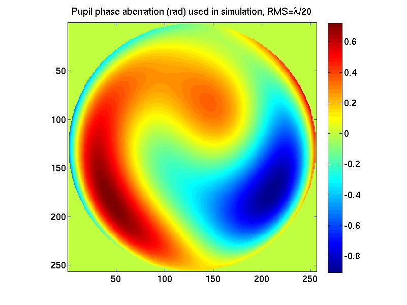
Figure 1: A common pixel response function for all the pixels used in the simulation (left) and low order phase aberration (right) in radian used in simulation with RMS $\sim\lambda/20$.

This pixel response function is roughly similar to the the intra-pixel variation for a backside-illuminated CCD[6]. We include $\lambda/20$ RMS low order wavefront aberrations parametrized by the first 15 Zernike polynomials, whose amplitudes are randomly generated. The right plot in Fig. 1 displays the phase aberration over the telescope pupil used in our simulation. The two plots (left for X centroid and right for Y centroid) in Fig. 2 displays the centroid estimation errors for a grid of X and Y offsets between the two images within range [-0.5, 0.5] pixel. These errors are due to truncation and are no more than 0.1 micro-pixel.

Figure 2: Centroid offset estimation errors X (left) and Y (right) in micro-pixel unit for an ideal CCD and wave front with $\lambda/20$ RMS low order aberrations parametrized by the first 15 Zernike polynomials. The pixel size is 10$\mu$m.

4.2 Pixel response calibration and results

For realistic detectors, pixel response functions vary from pixel to pixel, which we call inter-pixel variations. Pixel response calibration measures the pixel response functions of all the pixels. The Fourier transforms ${\tilde{Q}}_{mn}(k_{x},k_{y})$ of the pixel response functions $Q_{mn}(x,y)$ of all pixels are measured at various spatial frequencies. To do this, we illuminate the detector using a cosine intensity pattern. For NEAT, this is achieved by interfering two metrology lasers at various spatial frequencies . The fringe pattern gives a sinusoidal illumination on the pixel array and the separation of the two lasers determines the wavelengths of the fringes. AMO is used to offset the frequency of one laser from the other by a few Hz. The temporal variation of the pixel intensities are then used to estimate Fourier transforms ${\tilde{Q}}_{mn}(k_{x},k_{y})$ as discussed in section 3. We use expansion (14) to parametrize ${\tilde{Q}}_{mn}(k_{x},k_{y})$. For micro-arcsecond accuracy, we nominally keep the terms up to second order or third order in $k_{x}$ and $k_{y}$.

To simulate the inter-pixel response variations, we make the low order coefficients $c_{i}$ in Eq. (22) pixel dependent by replacing $c_{i}$ with $c_{i}+c_{i}^{\rm mn}$, where $c_{i}^{\rm mn}$ are random numbers drawn from zero mean Gaussian random number generators with standard deviation being 0.01. We also add 2% white noise to the pixel response as a multiplicative factor as well as random geometric pixel location shifts for all the pixels along both x and y directions with 0.01 pixel RMS. The left plot in Fig. 3 displays a typical intra pixel responses of a 10$\times$10 pixel array at the upper left corner of the 32$\times$32 array. Here the interpixel cross talk from diffusion is not displayed to avoid overlap. The zeroth order calibration measures the pixel response to a flat field, i.e. Fourier transform of the pixel response function at spatial wave number $(k_{x},k_{y})=(0,0)$. The right plot in Fig. 3 displays a typical flat field calibration results.

Figure 3: Simulated intrapixel detection variation for a 10$\times$10 array (left) and flat field response calibration result 32$\times$32 (right).

Fig. 4 shows systematic centroid displacement estimation errors with only flat field response calibration for different centroid offsets between the two images, whose range is [-0.5, 0.5] pixel along both x and y directions.

Figure 4: Centroid offset estimation errors X (left) and Y (right) in micro-pixel unit. The wavefront error is $\lambda/20$ specified by the first 15 Zernikes polynomials. Only a flat field calibration is applied.

The next level of calibration measures the effective pixel locations deviating from a regular grid. The effective location of pixel $(m,n)$ is estimated by fitting $\Delta x_{mn}k_{x}^{\rm met}+\Delta y_{mn}k_{y}^{\rm met}$ to the phase of the estimated Fourier transform ${\tilde{Q}}_{\rm mn}(k_{x}^{\rm met},k_{y}^{\rm met})$ at different values of spatial frequency $(k_{x}^{\rm met},k_{y}^{\rm met})$ available from the metrology system. Fig. 5 displays the estimated the effective pixel location deviating from a regular grid.

Figure 5: Effective pixel offsets along x (left) and y directions, the units are pixel

Now the errors shown in Fig. 6 are significantly reduced to tens of micro-pixels after including the effective pixel locations in estimation.

Figure 6: Centroid offset estimation errors X (left) and Y (right) in micro-pixel unit. The wavefront error is $\lambda/20$ specified by the first 15 Zernikes polynomials. A flat field and pixel effective location calibration is applied.

However, the errors are still large for micro-pixel level astrometry. We further include the second order amplitude terms in expansion (14) and estimate coefficients $\alpha_{mn},\beta_{mn}$, and $\gamma_{mn}$ by fitting expansion (14) to the estimated Fourier transforms ${\tilde{Q}}_{\rm mn}(k_{x}^{\rm met},k_{y}^{\rm met})$ at different values of $(k_{x}^{\rm met},k_{y}^{\rm met})$. The second order coefficients are displayed in Fig. 7.

Figure 7: Second order amplitudes $\alpha_{mn}$ (left), $\beta_{mn}$ (middle), and $\gamma_{mn}$ (right), coefficients for terms $k_{x}^{2},k_{y}^{2}$, and $k_{x}k_{y}$.

The two plots in Fig. 8 displays the centroid estimation errors for performing pixel response calibration that estimates the flat field response, the effective pixel locations, and the second order amplitude corrections.

Figure 8: Centroid offset estimation errors X (left) and Y (right) in micro-pixel unit. The wavefront error is $\lambda/20$ specified by the first 15 Zernikes polynomials. Calibration includes second order terms.

Including the third order terms in expansion (14) in our pixel response calibration enables us to achieve centroid estimation accuracy to be a few micro-pixels over [0.5, 0.5] pixel range along both x and y directions. The corresponding coefficients are displayed in Fig. 9.

Figure 9: Third order term coefficients, $ak_{x}^{3}$ (top, left), $bk_{x}^{2}k_{y}$ (top, right), $ck_{x}k_{y}^{2}$ (bottom, left), and $dk_{y}^{3}$ (bottom, right).

Fig. 10 shows systematic centroid displacement estimation errors for including through the third order phase terms. The RMS is only a few micro-pixels.

Figure 10: Centroid offset estimation errors X (left) and Y (right) in micro-pixel unit. The wavefront error is $\lambda/20$ specified by the first 15 Zernikes polynomials.

4.3 Noise sensitivity

So far, we have not included any noise. We now study the sensitivity to photon shot noise, which is the dominant source of random errors. We set the total number of photons for each image to be $10^{8}$ and use Poisson random number generator to simulate the photon shot noise. We simulated 1000 images with their centroid positions randomly distributed within $\pm$ 0.5 pixel relative to a reference image along both x and y directions. The reference image have the same level of photon and shot noise. Fig. 11 displays the Allan deviation of the estimated centroid displacements relative to a reference image as function of the total number of photons integrated. The green dash line shows an empirical sensitivity formula

$$\sigma\approx 1.5/\sqrt{N_{\rm ph}}$$ (23)

for uncertainty of centroid estimation using an equal weight in the least-squares fitting, where $N_{\rm ph}$ is the total number of photons. To reach 10 mirco-pixel precision, we shall need about 2.2$\times$10¹⁰ photons.

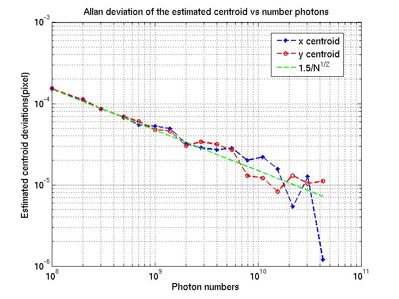
Figure 11: Centroid estimation error Allan deviations vs number of photons integrated.

The Allan deviation shows the variation between 1000 images with respect to the same reference image. How does the noise in the reference image affect the results? It turns out that the noise in the reference image causes mostly an overall offset to all the centroid displacements, or it is an excellent approximation that

$$d(A,R_{1})-d(B,R_{1})\approx d(A,R_{2})-d(B,R_{2})\,,$$ (24)

where $d(A,R_{1})$ represents the displacement of centroid of image A relative to reference image $R_{1}$ and so on. Fig. 12 shows the centroid displacements relative to two reference images, which are the same image with two different realization of photon noise. It is easy to see that the difference of the centroid displacements is insensitive to the uncertainties in the reference image( less than 1 micro-pixel).

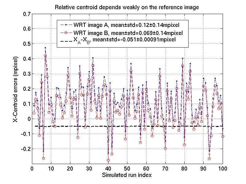
Figure 12: X centroid displacement error using reference image with different noise realizations.

We are performing an equal weight least-squares fitting, it is possible to optimize weights $W_{mn}$ to achieve the best sensitivity to noise, which will be a subject for future study.

4.4 Wave front stability

In this section, we study the sensitivity of our algorithm to wave front changes, i.e. the two images are taken with slightly different wavefront aberrations. The left plot in Fig. 13 shows a low order small wavefront change with $\lambda/1350$ RMS. (High order wave front aberrations generates speckles in the image plane while the low order wavefront change generates a change in the shape of the PSF. For PSF fitting, the centriod estimation is more sensitive to low order wavefront aberrations.) The main effect of a wavefront change between the two images is an overall constant, which is not a problem for differential astrometry. However, this overall constant depends on the pixel response functions. We shall need to show that this pixel dependency in the overall constant is small so that it is common for different portions of the detector. To do this, we instantiate a second detector whose pixel response function is slightly different from our nominal detector as a result of the random feature of our simulation.

The right plot in Fig. 13 shows the difference of the pixel responses between the two cameras which comes from the randomly instantiated low order polynomials.

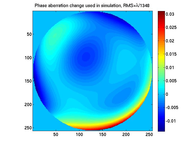
Figure 13: Pixel response difference between two detectors in a 10$\times$10 array (left). Wavefront variations between two observations, RMS $\sim\lambda/1350$, simulated by low order polynomials with randomly generated coefficients.

We now consider the case where the wavefront changes by an amount of $\lambda/1350$ RMS, as shown in the left plot in Fig. 13, between taking the two images whose centroid displacement we are interested to estimate. Fig. 14 displays the centroid displacement errors due to the $\lambda/1350$ RMS low order wavefront change for a grid of centroid offsets between the two images.

Figure 14: Centroid displacement estimation errors X (left) and Y (right) in micro-pixel unit. Both images are taken with a common low order wavefront error of $\lambda/20$ RMS specified by the first 15 Zernikes polynomials. The low order wavefront difference between the two images has RMS $\sim\lambda/1350$.

The main effect of a wavefront change between the two images is an overall constant independent of the actual displacement between the two images; the variation is only a few micro-pixels. If the overall constant is common for both stars, this effect cancels for differential astrometry.

Because the images of the two stars are at different locations in the focal plane array, we examine whether the different pixel response functions at different portions of the detector coupled with the wavefront change leads to significant error. Fig. 15 displays the centroid errors for using the second detector. To avoid common error cancellation, we put the reference image at [0.25, 0.25]pixel instead of [0, 0] pixel as for the first detector.

Figure 15: Centroid estimation errors X (left) and Y (right) in micro-pixel unit for the second detector. The images are taken with a common low order wavefront error of $\lambda/20$ RMS specified by the first 15 Zernikes polynomials and a differential low order wavefront error of RMS $\lambda/1350$.

Again, we can see that the dominant effect of wavefront change between the two images is an overall offset in the centroid estimation. Because the overall offset is not sensitive to the difference between two detectors, the overall differential displacement caused by the wavefront difference cancels leaving a residual of a few micro-pixel RMS. See Fig. 16.

Figure 16: The difference between the centroid displacement estimation errors X (left) and Y (right) in micro-pixel unit for two different simulated detectors. For each detector, the images are taken with a common low order wavefront error of $\lambda/20$ RMS specified by the first 15 Zernikes polynomials and a differential low order wavefront error of RMS $\lambda/1350$.

5 Polychromatic effect

In this section, we discuss the polychromatic effect. For white light source like stars, image intensity model (6) needs an extra integration over the photon wavelengths weighed with the source spectrum,

$$I_{mn}(x_{c},y_{c})=\int_{-\infty}^{\infty}\!dk_{x}\!\!\int_{-\infty}^{\infty}\!dk_{y}\int_{0}^{\infty}d\lambda S(\lambda){\cal I}(k_{x},k_{y},\lambda){\tilde{Q}}_{mn}\!(k_{x},k_{y},\lambda)e^{i\left[k_{x}((m{+}1/2)a{-}x_{c}){+}k_{y}((n{+}1/2)a{-}y_{c})\right]}$$ (25)

where $S(\lambda)$ is the source spectral energy density function and we have included the wavelength dependencies in Fourier transforms of the monochromatic PSF function ${\cal I}(k_{x},k_{y},\lambda)$ and the pixel detection function ${\tilde{Q}}_{mn}(k_{x},k_{y},\lambda)$. As a leading order approximation, we ignore the spectral dependency in the pixel detection function. The broadband image model has the same expression as the monochromatic model with the following replacement

$${\cal I}(k_{x},k_{y})\to\int_{0}^{\infty}d\lambda S(\lambda){\cal I}(k_{x},k_{y},\lambda)\,.$$ (26)

Because the integral over the photon wavelength is a linear operation, the polychromatic signal is still a bandwidth limited signal, whose bandwidth is determined by the shortest wavelength. As far as the pixelated images are Nyquist sampled, our algorithms works as for the case of monochromatic source. Fig. 17 displays the centroid offset estimation errors for simulated chromatic pixelated images pairs displaced by various offsets along x and y directions assuming an ideal tophat pixel response detection.

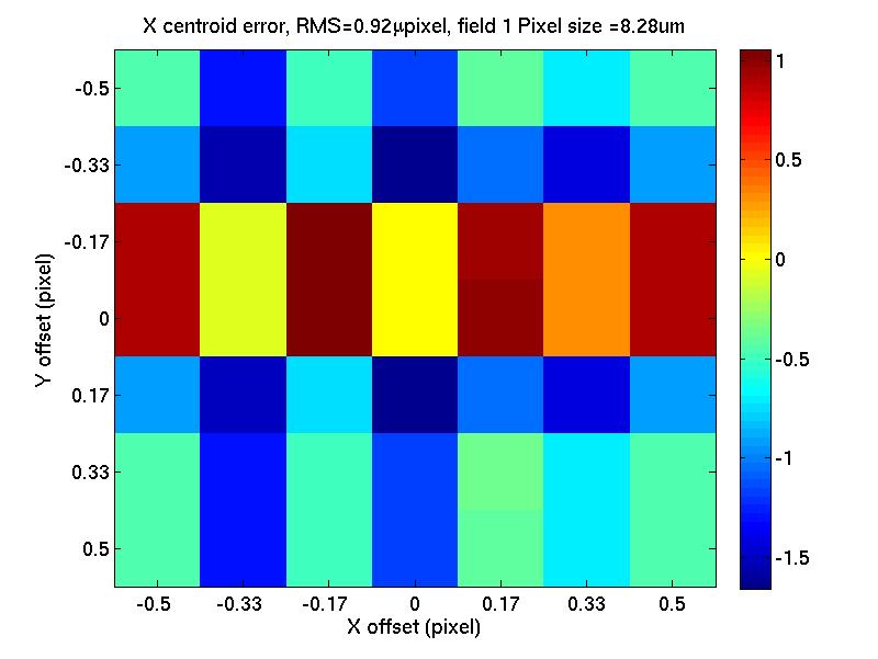
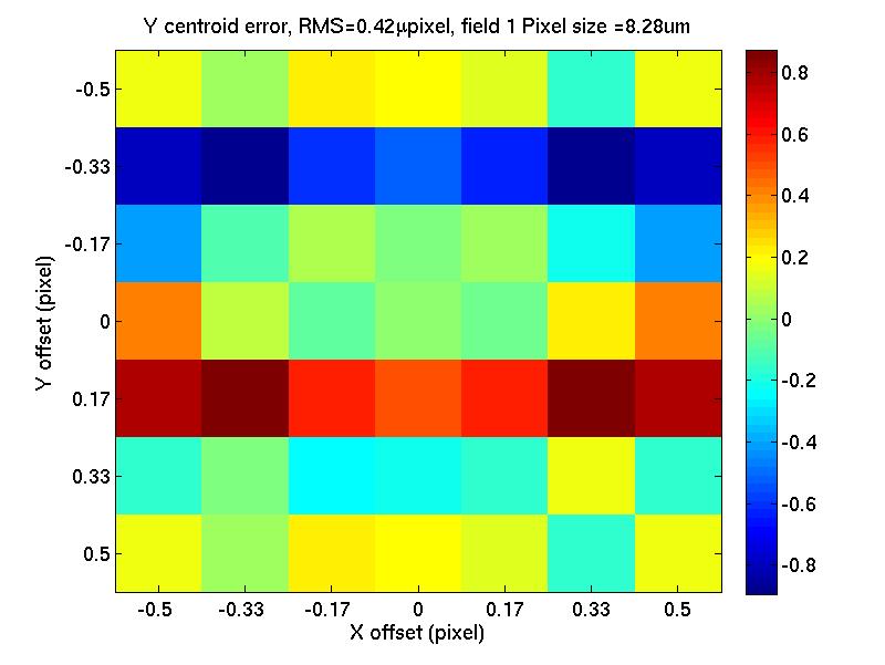
Figure 17: The estimation errors of the centroid offsets for broadband images.

We note that the error is sub-micro pixel. A slight complication comes from the dependency of pixel response on the wavelength, which requires pixel response calibration using metrology at multiple wavelengths. The results in reference[6] for backside illuminated CCD shows weak dependency on the wavelengths especially at the longer wavelength. Because we only need to calibrate the pixel to pixel variations of the pixel response functions, for differential astrometry, only the spectral dependency in the inter-pixel variations of the response functions coupled with the star spectral difference could cause systematic errors. We expect this effect to be small in general and can be calibrated using laser metrology at a few wavelengths. We defer the study of this to a future work.

6 Conclusions

We have presented a systematic frame work for accurate centroid displacement estimation and detector characterization. For an ideal detector with all the pixels having the same pixel response function, the PSF can be accurately reconstructed without any detector calibration. For realistic detectors whose pixel response functions share a dominant common portion and small pixel to pixel variations, it is possible to measure the pixel responses functions in Fourier space using laser metrology fringes. Measuring the pixel response in Fourier space is especially convenient for well sampled images. Keeping a few low order terms (e.g. 3rd order) in the Taylor series expansion of the Fourier transform in wave numbers, we can achieve centroid estimations accurate to a few micro-pixels. This enables micro-arcsecond level astrometry using telescope images of stars and thus detect earth-like exo-planets. This method is also applicable to precise photometry.

7 Acknowledgments

This work was prepared at the Jet Propulsion Laboratory, California Institute of Technology, under a contract with the National Aeronautics and Space Administration.

References

- [1] R. C. Stone, “A comparison of digital centering algorithms,” AJ, 97, 1227 (1989).
- [2] K. J. Mighell, “Stellar photometry and astrometry with discrete point spread functions,” MNRAS, 361, 861-878, (2005).
- [3] P. R. Jorden, J.-M. Deltron, and A. P. Oates, “The non-uniformity of CCD’s and the effects of spatial undersampling,” Proc. SPIE, 2198, 836 (1994).
- [4] D. Kavaldjiev and Z. Ninkov, “Subpixel sensitivity map for a charge-coupled device sensor,” Optical Engineering, 37, 948 (1998).
- [5] D. Kavaldjiev and Z. Ninkov, “Influence of nonuniform charge-coupled device pixel response on aperture photometry,” Optical Engineering, 40, 162 (2001).
- [6] A. Piterman and Z. Ninkov, “Subpixel sensitivity maps for a back-illuminated charge-coupled device and the effects of nonuniform response on measurement accuracy,” Optical Engineering, 41, 1192 (2002).
- [7] F. Malbet, et al, “High precision astrometry mission for the detection and characterization of nearby habitable planetary systems with the Nearby Earth Astrometric Telescope (NEAT),”, Proposal to the 2010 ESA Cosmic Vision call for M mission.