Two-dimensional kinematics of SLACS lenses – III.
Mass structure and dynamics of early-type lens galaxies beyond $z\simeq 0.1$

Abstract

We combine in a self-consistent way the constraints from both gravitational lensing and stellar kinematics to perform a detailed investigation of the internal mass distribution, amount of dark matter, and dynamical structure of the sixteen early-type lens galaxies from the SLACS Survey, at $z=0.08-0.33$, for which both HST/ACS and NICMOS high-resolution imaging and VLT VIMOS integral-field spectroscopy are available. Based on this data set, we analyze the inner regions of the galaxies, i.e. typically within one (three-dimensional) effective radius $r_{\mathrm{e}}$, under the assumption of axial symmetry and by constructing dynamical models supported by two-integral stellar distribution functions (DFs). For all systems, the total mass density distribution is found to be well approximated by a simple power-law $\rho_{\mathrm{tot}}\propto m^{-\gamma^{\prime}}$ (with $m$ being the ellipsoidal radius): this profile is on average slightly super-isothermal, with a logarithmic slope $\langle\gamma^{\prime}\rangle=2.074^{+0.043}_{-0.041}$ (errors indicate the 68% CL) and an intrinsic scatter $\sigma_{\gamma^{\prime}}=0.144^{+0.055}_{-0.014}$, and is fairly round, with an average axial ratio $\langle q\rangle=0.77\pm 0.04$. The lower limit for the dark matter fraction ($f_{\mathrm{DM}}$) inside $r_{\mathrm{e}}$ ranges, in individual systems, from nearly zero to almost a half, with a median value of 12%. By including stellar masses derived from stellar population synthesis (SPS) models with a Salpeter initial mass function (IMF), we obtain an average $f_{\mathrm{DM}}=31\%$, and the corresponding stellar profiles are physically acceptable, with the exception of two cases where they only marginally exceed the total mass profile. The $f_{\mathrm{DM}}$ rises to 61% if, instead, a Chabrier IMF is assumed. For both IMFs, the dark matter fraction increases with the total mass of the galaxy (correlation significant at the 3-sigma level). Based on the intrinsic angular momentum parameter calculated from our models, we find that the galaxies can be divided into two dynamically distinct groups, which are shown to correspond to the usual classes of the (observationally defined) slow and fast rotators. Overall, the SLACS systems are structurally and dynamically very similar to their nearby counterparts, indicating that the inner regions of early-type galaxies have undergone little, if any, evolution since redshift $z\approx 0.35$.

1 Introduction

Early-type galaxies are among the fundamental constituents of the local observable Universe, contributing to most of the total stellar mass (Fukugita, Hogan, & Peebles, 1998; Renzini, 2006), and it is therefore only natural that these systems have become the focus of a vast amount of observational and theoretical studies during recent years.

Understanding the formation and evolution mechanisms that can generate such a remarkably homogeneous class of objects remains among the most important open questions in present-day astrophysics: although the standard scenario according to which massive ellipticals are built-up via hierarchical merging of disk galaxies (see e.g Toomre, 1977; White & Frenk, 1991; Cole et al., 2000) has been steadily gaining consensus throughout the last decades, only recently the progress in high-resolution numerical simulations has allowed to start investigating in detail the internal structural properties of realistic systems (e.g. Meza et al. 2003, Naab et al. 2007, Jesseit et al. 2007, Oñorbe et al. 2007, González-García et al. 2009, Johansson, Naab, & Ostriker 2009, Lackner & Ostriker 2010).

Clearly, in view of these developments, the availability of stringent observational constraints has become even more crucial. Luckily, at least as far as nearby ellipticals are concerned, the observational and modelling effort has been very intense in the past few years. Stellar dynamics represents the most widely used diagnostic tool (see e.g. Saglia, Bertin, & Stiavelli 1992, Bertin et al. 1994, Franx et al. 1994, Carollo et al. 1995, Rix et al. 1997, Loewenstein & White 1999, Gerhard et al. 2001, Borriello et al. 2003, van den Bosch et al. 2008, Thomas et al. 2007, 2009, 2011 and in particular the SAURON project, de Zeeuw et al. 2002, and the Atlas3D project, Cappellari et al. 2010), although other studies have also successfully employed — sometimes in combination with stellar kinematics — different tracers such as planetary nebulae and globular cluster kinematics (e.g. Côté et al., 2003; Romanowsky et al., 2003, 2009; Coccato et al., 2009; de Lorenzi et al., 2009; Napolitano et al., 2009; Rodionov & Athanassoula, 2011), the occasional H I gas disk or ring (e.g. Oosterloo et al., 2002; Weijmans et al., 2008), and hot X-ray gas emission (e.g Matsushita et al., 1998; Fukazawa et al., 2006; Humphrey & Buote, 2010; Das et al., 2010; Churazov et al., 2010). In general, from these analyses there is mounting evidence that early-type galaxies are embedded in dark haloes, whose contribution is often significant already inside one effective radius, and that their total density profiles are roughly isothermal within the inner regions (but not necessarily at larger radii, see de Lorenzi et al. 2009, Dutton et al. 2010).

Ideally, if such studies could be extended to elliptical galaxies beyond the local Universe, it would become possible to provide strong constraints also to the intermediate steps of numerical simulations throughout redshift, rather than just to their $z=0$ end-products. The current observational limitations, unfortunately, make it prohibitively difficult to apply the traditional techniques to distant systems, i.e. at $z\approx 0.1$ and beyond. In particular, the impossibility to reliably measure the higher-order velocity moments needed to disentangle the mass–anisotropy degeneracy (Gerhard, 1993; van der Marel & Franx, 1993) constitutes a serious hindrance for dynamical studies. On the other hand, however, at higher redshifts strong gravitational lensing (see e.g. Schneider, Kochanek, & Wambsganss, 2006) may become available as an additional probe, opening up new possibilities to investigate the mass distribution of galaxies.

The main obstacle with this approach, namely the difficulty in discovering a suitable number of early-type galaxies that also act as strong gravitational lenses, has been remedied by the Sloan Lens ACS Survey, SLACS (Bolton et al. 2006, 2008a, 2008b, Koopmans et al. 2006, Treu et al. 2006, 2009, Gavazzi et al. 2007, 2008, Auger et al. 2009, 2010a), which has yielded a large sample of almost a hundred such objects. As highlighted by these studies, as well as by a number of other works (see Treu & Koopmans 2002, Koopmans & Treu 2003, Treu & Koopmans 2004, Rusin & Kochanek 2005, Jiang & Kochanek 2007, Grillo et al. 2008, Koopmans et al. 2009, Trott et al. 2010, van de Ven et al. 2010, Dutton et al. 2011, Spiniello et al. 2011), the combination of gravitational lensing and stellar dynamics provides a particularly powerful and robust method to determine the total mass density distribution of distant galaxies.

A potential limitation in the joint analysis of the SLACS galaxies mentioned above is that all the information about the dynamics is extracted from a single data point, i.e. the average stellar velocity dispersion measured within a 3 arcsec diameter aperture, obtained from SDSS spectra. Moreover, the method is not fully self-consistent, in the sense that axial symmetry is assumed for the lensing modelling, but not for the dynamical modelling, which is based on spherical Jeans equations. In order to address the concerns that these approximations might lead to biased results, the SLACS data set has been complemented, for about 30 lenses, with extended, two-dimensional kinematic information, obtained either with VLT VIMOS integral field unit (IFU) or from LRIS Keck long-slit spectroscopic observations (with the slit positions offset along the galaxy minor axis in order to mimic integral field capabilities). In addition, we have developed a more rigorous, self-consistent modelling technique (the cauldron code, based on the superposition of two-integral distribution functions, see Sect. 3 and Barnabè & Koopmans 2007), aimed at taking full advantage of the available data sets for each galaxy, namely the gravitationally lensed image, the surface brightness distribution and the velocity moments maps. This makes it possible to recover more accurate constraints on the slope and the flattening of the total mass density distribution, to derive information on the dark matter fraction within the inner regions and to obtain insights on the global and local dynamical status of the system, so that this analysis constitutes, to a good extent, the higher redshift analogue of the detailed studies that are routinely carried out on local ellipticals. We have applied this method to half a dozen SLACS galaxies with VIMOS observations (Czoske et al., 2008; Barnabè et al., 2009a), as well as to one of the Keck systems (Barnabè et al., 2010). In this paper, we extend this in-depth analysis to the full sample of SLACS early-type lenses with available VIMOS IFU spectroscopy (we refer to Czoske et al. 2011, in preparation, for a comprehensive description of the complete data set), a total of 16 systems at redshift $z=0.08$ to $0.35$, and covering a wide range in mass and angular momentum. We also make use of stellar masses derived from SPS models (Auger et al., 2009) to impose further constraints on the luminous distribution and estimate the contribution of the dark matter component.

This paper is organized as follows: in Section 2 we provide an overview of the available data-sets. In Section 3, after recalling the basic features of the method for the combined analysis of the adopted model, we present the main results of the study of the SLACS lenses mass density profiles. The mass structure of the analyzed galaxies, in terms of luminous and dark matter components, is described in Section 4, while Section 5 deals with the recovered dynamical structure of the systems. We discuss our findings in Section 6 and we briefly summarize the main conclusions in Section 7. Throughout this paper we adopt a concordance $\Lambda$CDM model described by $\Omega_{\mathrm{M}}=0.3$, $\Omega_{\Lambda}=0.7$ and $H_{0}=100\,h\,\mathrm{km\,s^{-1}\,Mpc^{-1}}$ with $h=0.7$, unless stated otherwise.

2 Observations

The joint lensing/dynamics analysis requires three types of input data: (i) high-resolution images are used to trace the surface brightness of the gravitationally lensed background galaxies; (ii) near-infrared images provide the surface brightness distribution of the stars in the lens galaxies; (iii) integral-field spectroscopic observations are used to derive two-dimensional maps of systematic velocity and velocity dispersion of the stars in the lens galaxies.

2.1 Imaging

High-resolution images of the lens systems in the sample were obtained with Advanced Camera for Surveys (ACS) on the Hubble Space Telescope (HST). We use images taken through the F814W filter. Deep images are available for eight of the systems, while for the remaining nine only single-exposure snapshot images are available. The pixel scale of the images is $0.05\,\mathrm{arcsec}$. The structure of the gravitationally lensed background images was isolated by subtracting elliptical B-spline models of the lens galaxies’ light distribution (Bolton et al., 2008a).

NICMOS F160W images were used to obtain the surface brightness of the lens galaxies. In order to serve as luminosity weights to the kinematic maps, the images were matched in resolution to the spectroscopic observations ($0.8\,\mathrm{arcsec}$) and resampled from the original pixel scale of $0.05\,\mathrm{arcsec}$ to the pixel grid of the kinematic maps ($0.67\,\mathrm{arcsec}$). For three systems no NICMOS observations were available. In these cases, the lens surface brightness was obtained from the B-spline fits to the F814W images.

2.2 Spectroscopy

Two-dimensional spectroscopy of seventeen systems was obtained with the integral-field unit of VIMOS on the VLT. Three systems (J0037, J0912 and J2321) were observed with the HR-Blue grism($4000-6200$ Å) , while the remainder were observed with the HR-Orange grism ($5000-7500$ Å). The field of view of $27\arcsec\times 27\arcsec$ was sampled with $40\times 40$ spatial elements with a scale of $0.67\,\mathrm{arcsec}$, the spectral resolution is $R\approx 2500$ (corresponding to a velocity resolution of $\Delta v\approx 90-110\,\mathrm{km\,s^{-1}}$ FWHM in the rest frame of the lens galaxies). Two-dimensional maps of systematic velocity (with respect to the mean redshift of the lens galaxy) and velocity dispersion were measured by fitting stellar templates convolved with Gaussian line-of-sight velocity distributions to the spectra from spatial elements with a sufficient signal-to-noise ratio ($S/N>8$ per spectral element of $0.644$ Å).

A full description of the sample, observations, data reduction and the resulting kinematic maps is given in a companion paper (Czoske et al. 2011, in preparation).

3 Combined lensing and dynamics analysis

In this Section — after recalling the adopted modelling assumptions and the salient features of the method employed to self-consistently combine lensing and dynamics constraints — we present the core results of the study of the full sample of sixteen SLACS early-type lens galaxies for which data sets including both high-resolution imaging and VIMOS integral field spectroscopy are available.

The theoretical framework of the joint lensing and dynamics analysis and the implementation of the method (i.e., the cauldron code) are described in full detail in Barnabè & Koopmans (2007, hereafter BK07), to which we refer the interested reader.

3.1 Method overview

We describe the total mass density distribution of the lens galaxy as $\rho(\mn@boldsymbol{x};\mn@boldsymbol{\eta})$, where the vector $\mn@boldsymbol{x}$ denotes the spatial coordinates and $\mn@boldsymbol{\eta}$ is a set of parameters that characterizes the density profile. The corresponding total gravitational potential, $\Phi(\mn@boldsymbol{x})$, is calculated via the Poisson equation and utilized for both the gravitational lensing and the stellar dynamics modelling of the data set. By employing a pixelated source reconstruction method (see e.g. Warren & Dye 2003, Koopmans 2005, Suyu et al. 2006) for the lensing and some flavour of the Schwarzschild orbit superposition method (Schwarzschild 1979; see Thomas 2010 for a review of the developments of this technique) for the dynamics, both these modelling problems can be formally written in an analogous way as a set of regularized linear equations, for which robust solving techniques are readily available (see e.g. Press et al., 1992).

Clearly, for any given set of observations, the ultimate goal of the analysis is to determine the set of $\mn@boldsymbol{\eta}$ parameters that generate the ‘best’ density model, i.e. the most plausible in an Occam’s razor sense. This can be achieved by embedding the linear optimization scheme within the framework of Bayesian inference, which provides an objective way to quantify the probability of each model given the data (see e.g. MacKay, 1999, 2003). The best model is thus the maximum a posteriori (MAP) model, i.e. the one that maximizes the joint posterior probability density function (PDF).

While this method is very general, allowing in principle for any density distribution, in its current implementation — the cauldron algorithm — we make further assumptions in order to achieve the computational efficiency that is needed for a thorough exploration of the parameter space. Within the cauldron code, therefore, galaxies are modelled as axially symmetric systems, i.e. $\rho(R,z)$, whose dynamics are described by a two-integral distribution function (DF) $f=f(E,L_{z})$ which depends on the two classical integrals of motions, the energy $E$ and the angular momentum along the rotation axis $L_{z}$. This makes it possible to construct dynamical models in a matter of seconds, by means of a fast Monte Carlo numerical implementation developed by BK07 of the two-integral Schwarzschild method originally introduced by Cretton et al. (1999) and Verolme & de Zeeuw (2002), which employs two-integral components (TICs), rather than the commonly used stellar orbits, as dynamical building blocks. TICs can be viewed as elementary stellar systems completely specified by a particular choice of $E$ and $L_{z}$; they are characterized by analytic radial density distributions and (unprojected) velocity moments, which makes them convenient and (compared to orbits) computationally inexpensive building blocks.

Remarkably, the applicability of the code is not too severely limited by the assumptions mentioned above: as shown in Barnabè et al. (2009a), cauldron has been successfully tested for robustness by applying it to a complex system obtained from a numerical N-body simulation of a merger process, which obviously departs from the condition of axisymmetry. Nevertheless, several important global properties of the system (particularly the total density slope and, when rotation is visible in the kinematics maps, the angular momentum and the ratio of ordered to random motions) are recovered quite reliably, typically within 10 to 25 per cent of the true value.

3.2 The galaxy model

We model the total mass density profile of the lens galaxy with an axially symmetric power-law distribution,

$$\rho(m)=\frac{\rho_{0}}{m^{\gamma^{\prime}}},$$ (1)

where $\rho_{0}$ is a density scale, $\gamma^{\prime}$ is the logarithmic slope of the profile, and the ellipsoidal radius $m$ is defined as

$$m^{2}\equiv\frac{R^{2}}{a_{0}^{2}}+\frac{z^{2}}{a_{0}^{2}q^{2}};$$ (2)

here $a_{0}$ denotes the arbitrary length-scale and $q$ is the axial ratio ($q=1$ for a spherical galaxy, while oblate systems have $0\leq q<1$). The corresponding gravitational potential is obtained by applying the Chandrasekhar (1969) formula for homoeoidal density distributions and can be written as a rather simple expression (cf. Barnabè et al., 2009a) that just requires the computation of a one-dimensional integral.

Despite its simplicity, the power-law model (typically with a slope close to the isothermal case, i.e. $\gamma^{\prime}=2$) provides a good description of the total mass distribution of early-type galaxies over a large radial range, as reported by previous analyses of the SLACS systems (Koopmans et al., 2006; Gavazzi et al., 2007; Czoske et al., 2008; Barnabè et al., 2009a; Koopmans et al., 2009; Auger et al., 2010a), as well as a number of stellar dynamics (e.g. Gerhard et al., 2001), gravitational lensing (e.g. Dye et al., 2008; Tu et al., 2009) and X-ray studies (e.g. Humphrey & Buote, 2010) of ellipticals.

Three physical parameters (the non-linear parameters $\mn@boldsymbol{\eta}$, in the notation of Sect. 3.1) characterize the power-law model: the logarithmic density slope $\gamma^{\prime}$, the axial ratio $q$ and the lens strength $\alpha_{0}$, a dimensionless quantity directly related to the normalization of the potential well (see Appendix B of BK07). Furthermore, four ‘geometrical’ parameters are needed to describe the observed configuration of the lens galaxy in the sky, i.e. the inclination angle $i$ (with $i=90^{\circ}$ being an edge-on system), the position angle and the sky-coordinates of the centre of the system. Luckily, the last three parameters are well constrained by the surface brightness distribution of the lens galaxy and of the lensed images. Therefore, after determining their values by means of fast preliminary explorations, we maintain them fixed during the computationally expensive optimization and error analysis runs.

The level of regularization, which controls the smoothness in the reconstructed background source and TIC weight maps, is set through three additional non-linear parameters, usually known as hyper-parameters (see Suyu et al. 2006 and BK07 for a more technical explanation). The optimal values of the hyper-parameters are also found via maximization of the joint posterior PDF.

3.3 Bayesian inference and uncertainties

For our analysis we follow the standard Bayesian framework described by, e.g., MacKay (2003) involving multiple levels of inference; here we summarize the main steps involved in this approach, referring the interested reader to BK07 for a detailed explanation of the method.

Let us denote the combined data set as $\mn@boldsymbol{d}$, the noise in the data as $\mn@boldsymbol{n}$ and the considered hypothesis (i.e. the adopted model) as $\mathcal{H}$($\mn@boldsymbol{\eta}$), where the non-linear parameters $\mn@boldsymbol{\eta}$ are the physical and geometrical quantities (such as the density slope, axial ratio, lens strength and inclination angle) that characterize the model. At the first level of inference, the model is assumed to be true (i.e. we fix one choice for the set of $\mn@boldsymbol{\eta}$ parameters) and we aim to solve for $\mn@boldsymbol{w}$ the linear problem

$$\mn@boldsymbol{d}=\mathbf{A}\mn@boldsymbol{w}+\mn@boldsymbol{n}\,,$$ (3)

where $\mn@boldsymbol{w}$ are the linear parameters — namely, the surface brightness distribution of the lensed background source and the weights of the dynamical building blocks — being mapped onto the observables by the operator $\mathbf{A}=\mathbf{A}[\mathcal{H}(\mn@boldsymbol{\eta})]$. The construction of the mapping operator $\mathbf{A}$ for both the lensing and dynamics modelling constitutes the core of the cauldron code, and is described in BK07. From Bayes’ theorem, the posterior probability of the parameters $\mn@boldsymbol{w}$ given the data is written as

$$\mathrm{Pr}(\mn@boldsymbol{w}\,|\,\mn@boldsymbol{d},\mu,\mn@boldsymbol{\eta})=\frac{\mathrm{Pr}(\mn@boldsymbol{d}\,|\,\mn@boldsymbol{w},\mn@boldsymbol{\eta})\,\mathrm{Pr}(\mn@boldsymbol{w}\,|\,\mu)}{Z_{1}}\,,$$ (4)

where the probability $\mathrm{Pr}(\mn@boldsymbol{d}\,|\,\mn@boldsymbol{w},\mn@boldsymbol{\eta})$ is the likelihood and $\mathrm{Pr}(\mn@boldsymbol{d}\,|\,\mn@boldsymbol{w},\mn@boldsymbol{\eta})$ represents the prior. Here, we adopt as prior a curvature regularization function that describes the degree of smoothness that we expect to find in the solution; the amount of regularization to be applied is set by the value of the so-called ‘hyper-parameter’ $\mu$. The evidence $Z_{1}=\mathrm{Pr}(\mn@boldsymbol{d}\,|\,\mu,\mn@boldsymbol{\eta})=\int\mathrm{Pr}(\mn@boldsymbol{d}\,|\,\mn@boldsymbol{w},\mn@boldsymbol{\eta})\,\mathrm{Pr}(\mn@boldsymbol{w}\,|\,\mu)\,\mathrm{d}\mn@boldsymbol{w}$ is simply a normalization constant in Eq. (4), but it becomes important at the upper level of inference, where it appears as the likelihood. The set of parameters $\mn@boldsymbol{w}_{\mathrm{MAP}}$ that maximizes the posterior can be obtained by means of standard linear optimization techniques.

Analogously, at the second level of inference the $\mn@boldsymbol{\eta}$ parameters are still maintained fixed and the posterior probability of the hyper-parameter is

$$\mathrm{Pr}(\mu\,|\,\mn@boldsymbol{d},\mn@boldsymbol{\eta})=\frac{\mathrm{Pr}(\mn@boldsymbol{d}\,|\,\mu,\mn@boldsymbol{\eta})\,\mathrm{Pr}(\mu)}{Z_{2}}\,;$$ (5)

here we adopt a scale invariant prior $\mathrm{Pr}(\mu)\propto 1/\mu$ (uniform in log) to formalize our ignorance of the order of magnitude of the hyper-parameter.

Finally, at the third level of inference we can compare the different models by studying the posterior probability distribution of the set of non-linear parameters $\mn@boldsymbol{\eta}$,

$$\mathrm{Pr}(\mn@boldsymbol{\eta}\,|\,\mn@boldsymbol{d})=\frac{\mathrm{Pr}(\mn@boldsymbol{d}\,|\,\mn@boldsymbol{\eta})\,\mathrm{Pr}(\mn@boldsymbol{\eta})}{Z_{3}}\,,$$ (6)

and infer the parameters $\mn@boldsymbol{\eta}_{\mathrm{MAP}}$ for which the posterior is maximized. For each galaxy, the corresponding MAP model constitutes the ‘best model’, meaning the most plausible joint set of model parameters given the data, and therefore throughout the paper we present the reconstructed observables, background source, TIC weights maps and inferred quantities that are obtained with the choice $\mn@boldsymbol{\eta}=\mn@boldsymbol{\eta}_{\mathrm{MAP}}$. As prior function $\mathrm{Pr}(\mn@boldsymbol{\eta})$, we initially adopt very broad uninformative uniform priors: for the logarithmic slope we consider the interval $\gamma\in[1,3]$; for the lens strength $\alpha_{0}\in[0,1]$; the inclination can assume all the values $i\in[0^{\circ},90^{\circ}]$; finally, the axial ratio $q\in[0,1.5]$ can account for all the flattenings between a thin disk and a very prolate distribution. Fast preliminary exploration runs then permit us to select, for each system, narrower priors that remain, however, generously non-restrictive (i.e. they contain the bulk of the posterior and a wide margin of safety all around it).

The uncertainties on each individual parameter $\eta_{k}$ are obtained by marginalizing the posterior PDF over all other parameters. We refer to the parameter value that corresponds to the maximum of the $k$-th one-dimensional marginalized distribution as $\eta_{k,\mathrm{max}}$. In this context, it is important to note that, in general, $\mn@boldsymbol{\eta}_{\mathrm{MAP}}$ and $\mn@boldsymbol{\eta}_{\mathrm{max}}$ do not coincide and can actually differ significantly. In other words, the MAP parameters individually are not guaranteed to be probable: although the MAP solution corresponds by definition to the highest value of the joint posterior PDF, it does not necessarily occupy a large volume in the multivariate parameter space and could easily lie outside of the bulk of the posterior PDF if the distribution is strongly non-symmetric.

The computationally expensive task of exploring the posterior distribution $\mathrm{Pr}(\mn@boldsymbol{\eta}\,|\,\mn@boldsymbol{d})$ is accomplished by making use of the very efficient and robust MultiNest algorithm (Feroz & Hobson, 2008; Feroz et al., 2009), which implements the ‘nested sampling’ Monte Carlo technique (Skilling, 2004; Sivia & Skilling, 2006), and can provide reliable posterior inferences even in presence of multi-modal and degenerate multivariate distributions. For the analysis of the SLACS lenses, we launch MultiNest with 200 live points (the live or active points are the initial samples, drawn from the prior distribution, from which the posterior exploration is started) to obtain the individual marginalized posterior PDFs of the non-linear parameters $i$, $\alpha_{0}$, $\gamma$ and $q$. In the following, unless stated otherwise, we quote the 99 per cent confidence intervals (calculated such that the probability of being below the interval is the same as being above it) obtained from these distributions as our uncertainty on the parameters.

Table 1: Recovered parameters for the sixteen sample SLACS lens galaxies.

Galaxy name	$z_{\mathrm{lens}}$	$z_{\mathrm{src}}$	$\eta_{\mathrm{MAP}}$					$\eta_{\mathrm{max}}$
			$\gamma^{\prime}$	$\alpha_{0}$	$q$	$i$		$\gamma^{\prime}$	$\alpha_{0}$	$q$	$i$
SDSS J0037$-$0942	0.1955	0.6322	1.968	0.434	0.693	65.5		$1.969^{+0.014}_{-0.051}$	$0.433^{+0.018}_{-0.009}$	$0.694^{+0.047}_{-0.041}$	$65.4^{+2.6}_{-0.9}$
SDSS J0216$-$0813	0.3317	0.5235	1.973	0.344	0.816	70.0		$1.972^{+0.035}_{-0.077}$	$0.344^{+0.018}_{-0.012}$	$0.818^{+0.065}_{-0.061}$	$69.5^{+6.3}_{-2.2}$
SDSS J0912$+$0029	0.1642	0.3240	1.877	0.412	0.672	87.8		$1.880^{+0.035}_{-0.016}$	$0.413^{+0.005}_{-0.004}$	$0.670^{+0.021}_{-0.026}$	$87.6^{+0.4}_{-1.6}$
SDSS J0935$-$0003	0.3475	0.4670	2.285	0.225	0.982	34.8		$2.280^{+0.072}_{-0.056}$	$0.228^{+0.013}_{-0.019}$	$0.982^{+0.033}_{-0.124}$	$34.0^{+2.3}_{-2.8}$
SDSS J0959$+$0410	0.1260	0.5349	1.873	0.323	0.930	80.4		$1.869^{+0.013}_{-0.024}$	$0.325^{+0.009}_{-0.008}$	$0.920^{+0.029}_{-0.035}$	$80.8^{+1.9}_{-1.5}$
SDSS J1204$+$0358	0.1644	0.6307	2.226	0.399	1.000	65.2		$2.223^{+0.057}_{-0.074}$	$0.382^{+0.020}_{-0.011}$	$0.986^{+0.028}_{-0.104}$	$65.8^{+6.3}_{-3.4}$
SDSS J1250$+$0523	0.2318	0.7953	2.131	0.339	0.771	29.1		$2.134^{+0.025}_{-0.074}$	$0.336^{+0.021}_{-0.011}$	$0.772^{+0.054}_{-0.133}$	$28.4^{+3.9}_{-6.0}$
SDSS J1251$-$0208	0.2243	0.7843	1.925	0.244	0.796	85.6		$1.924^{+0.009}_{-0.030}$	$0.245^{+0.005}_{-0.006}$	$0.805^{+0.018}_{-0.046}$	$85.4^{+1.6}_{-2.9}$
SDSS J1330$-$0148	0.0808	0.7115	2.276	0.155	0.414	74.3		$2.280^{+0.039}_{-0.037}$	$0.154^{+0.008}_{-0.012}$	$0.414^{+0.018}_{-0.073}$	$75.3^{+1.9}_{-1.7}$
SDSS J1443$+$0304	0.1338	0.4187	2.435	0.149	0.698	71.5		$2.431^{+0.069}_{-0.076}$	$0.150^{+0.020}_{-0.021}$	$0.682^{+0.042}_{-0.085}$	$71.8^{+2.5}_{-1.0}$
SDSS J1451$-$0239	0.1254	0.5203	2.053	0.332	0.999	40.8		$2.028^{+0.030}_{-0.019}$	$0.337^{+0.003}_{-0.007}$	$0.997^{+0.012}_{-0.055}$	$40.8^{+1.9}_{-3.0}$
SDSS J1627$-$0053	0.2076	0.5241	2.122	0.369	0.851	56.4		$2.123^{+0.029}_{-0.016}$	$0.369^{+0.004}_{-0.011}$	$0.853^{+0.014}_{-0.040}$	$55.8^{+1.1}_{-1.2}$
SDSS J2238$-$0754	0.1371	0.7126	2.088	0.362	0.781	79.8		$2.098^{+0.022}_{-0.053}$	$0.358^{+0.011}_{-0.005}$	$0.767^{+0.042}_{-0.067}$	$79.1^{+1.1}_{-2.2}$
SDSS J2300$+$0022	0.2285	0.4635	1.921	0.349	0.642	59.4		$1.923^{+0.033}_{-0.043}$	$0.344^{+0.007}_{-0.004}$	$0.622^{+0.034}_{-0.012}$	$58.7^{+4.0}_{-1.9}$
SDSS J2303$+$1422	0.1553	0.5170	2.102	0.436	0.642	89.1		$2.098^{+0.030}_{-0.004}$	$0.437^{+0.003}_{-0.007}$	$0.644^{+0.004}_{-0.033}$	$85.9^{+3.5}_{-0.8}$
SDSS J2321$-$0939	0.0819	0.5324	2.058	0.467	0.744	67.3		$2.059^{+0.013}_{-0.066}$	$0.468^{+0.009}_{-0.003}$	$0.744^{+0.029}_{-0.011}$	$67.5^{+2.1}_{-2.0}$

Note. The non-linear $\eta$ parameters are: the logarithmic slope $\gamma^{\prime}$; the dimensionless lens strength $\alpha_{0}$; the axial ratio $q$ and the inclination $i$ (in degrees) with respect to the line-of-sight. Columns 4 to 7 list the MAP parameters, i.e. the parameters that maximize the joint posterior distribution (‘best model’ parameters). Columns 8 to 11 encapsulate a description of the one-dimensional marginalized posterior PDFs (shown as histograms in Appendix B in the online version of the journal): $\eta_{\mathrm{max}}$ is the maximum of that distribution and the indicated errors represent the lower and upper limits of the 99 per cent confidence interval.

3.4 Results

The cauldron code has been applied to the analysis of all sixteen lens galaxies for which VIMOS integral-field spectroscopic data are available. These objects are all early-type galaxies, with the exception of J1251$-$0208, which is morphologically classified by Auger et al. (2009) as a late-type galaxy. We include the latter in the E/S0 sample studied in this paper, since it is a bulge-dominated system which was spectroscopically selected from the SDSS using the same criteria — optimized to detect bright early-type lens galaxies — adopted for the other objects (see Bolton et al., 2005, 2006). For six of the systems, the results of the combined lensing and dynamics study were reported in previous publications (Czoske et al., 2008; Barnabè et al., 2009a). However, updated and extended kinematic maps are available for J2321 and therefore we have re-analyzed that galaxy.

Table 1 lists, for each galaxy, the recovered non-linear parameters for the MAP model, i.e. the inclination $i$, the lens strength $\alpha_{0}$, the logarithmic slope $\gamma^{\prime}$ and the axial ratio $q$ of the total density distribution. The reconstructed observables corresponding to this model are presented and compared to the data sets in Appendix A (available in the online version of the journal), where also the recovered unlensed background source is shown; the MAP model reconstruction of the weighted DF is presented in Sect. 5, where we study the dynamical structure of the lens galaxies. None of the galaxies requires external shear to be added to the model.

The marginalized posterior PDFs for the non-linear model parameters — which quantify the statistical uncertainties on those parameters (see Sect. 3.3) — are presented in Appendix B (available in the online version of the journal) for all sixteen galaxies in the sample. In Table 1 we also indicate, as a compact description of the errors, the parameter values which correspond to the maximum of the marginalized posterior distributions (subscript ‘max’) and the limits of the 99 per cent confidence intervals.

All the observables are, in general, accurately reproduced within the noise level. In particular, the lensed image residual maps do not exhibit the prominent structured patterns that can be seen when the method is applied to complex simulated systems, as in the Barnabè et al. (2009b) tests, thus indicating that the underlying density distribution of real ellipticals is fairly smooth and well-behaved, and can be satisfactorily modelled by the axisymmetric power-law profile of Eq. (1).

The reconstructed background sources generally appear as simple and smooth systems dominated by a single component, but a few of them display a more complex morphology or fainter secondary components. To understand this, we recall that the SLACS candidates are spectroscopically selected from the SDSS database by identifying those systems which have composite spectra consisting of both an absorption-dominated continuum (due to the foreground galaxy) and multiple nebular emission lines at a higher redshift (due to the background object), which directly trace star formation (see Bolton et al., 2006). Therefore, the background objects tend to be actively star-forming galaxies which, in the typical redshift range where the sources are located, i.e. $0.4\lesssim z\lesssim 0.8$, can sometimes be late-type systems characterized by clumpy, irregular and flocculent appearances (cf. e.g. Zamojski et al., 2007; Elmegreen et al., 2009).

The complicated and patchy morphology of certain sources (as in the case of SDSS J2303 or, more conspicuously, of the SLACS lens SDSS J0728 analyzed in Barnabè et al. 2010) as well as the presence of multiple sources almost adjacent to each other (e.g. SDSS J1251, SDSS J2321) can thus be interpreted as distinct star-forming regions within the same galaxy. Analogously, the small clumps observed in SDSS J1250 can likely be identified as bright blue star-forming regions that are observed within an interacting system with a tidal tale.

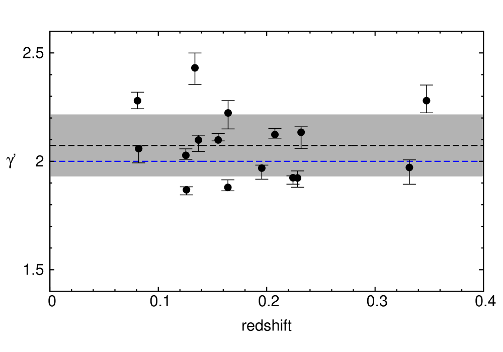
Figure 1: The logarithmic slope of the total density profile plotted against redshift for the sixteen early-type lens galaxies in the ensemble. The error bars are calculated by considering the region of the marginalized posterior PDF for $\gamma^{\prime}$ (see Figure 34) which contains 99 per cent of the probability. The blue line indicates the slope $\gamma^{\prime}=2$, corresponding to the isothermal profile, while the dashed black line denotes the average slope $\langle\gamma^{\prime}\rangle=2.07$ for the sample. The grey band region visualizes the intrinsic scatter of about 7 per cent in $\gamma^{\prime}$ (see text for details).

Figure 2: Joint posterior probability for $\gamma^{\prime}_{\mathrm{c}}$ and $\sigma_{\gamma^{\prime}}$ (see Eq. [7]). The cross marks the position of the joint maximum. The three contours correspond to the posterior ratios $\mathcal{P}/\mathcal{P_{\mathrm{max}}}=e^{-\Delta\tilde{\chi}^{2}/2}$, with $\Delta\tilde{\chi}^{2}=1,4,9$. The contours are only for indication: formally, they can be interpreted as 1, 2 and 3 $\sigma$ contours only for a (multivariate) Gaussian distribution, in which case $\tilde{\chi}^{2}$ represents the usual chi-square.

3.4.1 The slope of the density profile

By examining the recovered values for the logarithmic slope of the total density distribution, we find no evidence of evolution of $\gamma^{\prime}$ with redshift within the probed range ($z=0.08$ to $0.35$), confirming the results of Koopmans et al. (2009) and Auger et al. (2010a) on the full SLACS sample (see Figure 1). Moreover, from the same Figure, we also see that, while almost all systems have a nearly (i.e. within 10 per cent) isothermal profile, very few of them exhibit a slope that is actually consistent with $\gamma^{\prime}=2$ within the uncertainties.

We now proceed to study in a more quantitative way the distribution of density slopes for the ensemble at hand. Under the assumption that the slope $\gamma^{\prime}_{\mathrm{i}}$ (with a symmetrized 1 $\sigma$ error $\delta{\gamma^{\prime}_{\mathrm{i}}}$) of each lens system is drawn from a parent Gaussian distribution of centre $\gamma^{\prime}_{\mathrm{c}}$ and standard deviation $\sigma_{\gamma^{\prime}}$, the joint posterior probability $\mathcal{P}$ of these two parameters for the sample is given by

$$\mathcal{P}=\mathrm{Pr}(\gamma^{\prime}_{\mathrm{c}},\sigma_{\gamma^{\prime}}\,|\,\{\gamma^{\prime}_{\mathrm{i}}\})\propto p(\gamma^{\prime}_{\mathrm{c}},\sigma_{\gamma^{\prime}})\,\prod_{\mathrm{i}}\frac{\exp{\left[-\frac{(\gamma^{\prime}_{\mathrm{i}}-\gamma^{\prime}_{\mathrm{c}})^{2}}{2({\sigma_{\gamma^{\prime}}^{2}}+\delta{\gamma^{\prime}_{\mathrm{i}}}^{2})}\right]}}{\sqrt{2\pi({\sigma_{\gamma^{\prime}}^{2}}+\delta{\gamma^{\prime}_{\mathrm{i}}}^{2})}}\,,$$ (7)

where $p(\gamma^{\prime}_{\mathrm{c}},\sigma_{\gamma^{\prime}})$ indicates the prior, for which we adopt a uniform distribution. This probability function, visualized in Figure 2, yields the average logarithmic density slope

$$\langle\gamma^{\prime}\rangle=2.074^{+0.043}_{-0.041}\quad(68\%\;\mathrm{CL}),$$

which is slightly super-isothermal. This result is consistent with the value of $\langle\gamma^{\prime}\rangle$ determined by the Koopmans et al. (2009) and Auger et al. (2010a) combined lensing and dynamics analysis of the full SLACS sample (which does not include two-dimensional kinematic information), using spherical Jeans equations and assuming an isotropic stellar velocity dispersion tensor.

The intrinsic scatter around the average slope, also derived from the posterior distribution of Eq. (7), is

$$\sigma_{\gamma^{\prime}}=0.144^{+0.055}_{-0.014}\quad(68\%\;\mathrm{CL}),$$

which corresponds to $6.9^{+2.7}_{-0.6}$ per cent of $\langle\gamma^{\prime}\rangle$, and is displayed in Figure 1 as a grey band. This value is only marginally lower than the intrinsic scatter of about 10 per cent obtained by Koopmans et al. (2009) and Auger et al. (2010a), and the two $\sigma_{\gamma^{\prime}}$ are consistent within the errors.

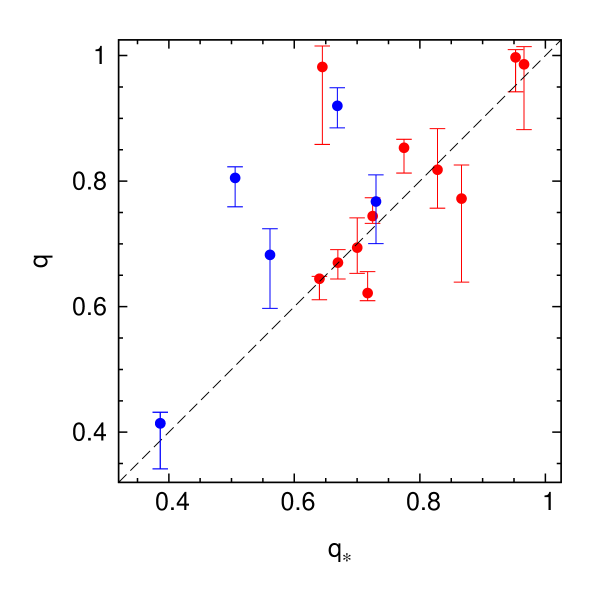
Figure 3: Axial ratio $q$ of the total density distribution plotted against the intrinsic axial ratio $q_{\ast}$ of the luminous distribution. For each galaxy, $q_{\ast}$ is calculated by deprojecting the observed isophotal axis ratio $q_{\mathrm{\ast,2D}}$, using the recovered MAP value of the inclination. The dashed line corresponds to $q=q_{\ast}$. Red and blue symbols denote, respectively, slow and fast rotators.

3.4.2 The flattening of the density profile

All the analyzed galaxies — with the exception of SDSS J1330 — are found to be in the range between moderately flattened and perfectly spherical, with a total density axial ratio $0.6<q\leq 1.0$. The ensemble-average axial ratio, obtained from the joint posterior probability as described in Sect. 3.4.1, is

$$\langle q\rangle=0.770^{+0.042}_{-0.041}\quad(68\%\;\mathrm{CL}),$$

with a quite substantial intrinsic scatter of about 19 per cent around this value:

$$\sigma_{q}=0.148^{+0.049}_{-0.019}\quad(68\%\;\mathrm{CL}).$$

The three roundest galaxies in the sample, and the only ones consistent with being spherical, are all slow rotators (see Emsellem et al. 2007, and Sect. 5.2 for our definition of slow and fast rotating systems based on the specific angular momentum). The system SDSS J1330, which is peculiar for its remarkably flattened axial ratio $q\simeq 0.4$, also bears the distinction of being the least massive object and one of the only five fast-rotating galaxies in the sample. Fast rotators, however, are not necessarily very flattened: SDSS J0959, for instance, is found to be almost spherical, with $q=0.9$.

In Figure 3, $q$ is compared to the intrinsic (i.e. three-dimensional) axial ratio of the luminous distributions, $q_{\ast}$, calculated as

$$q_{\ast}=\sqrt{1-(1-q^{2}_{\mathrm{\ast,2D}})/{\sin}^{2}i}\>\textrm{,}$$ (8)

where $q_{\mathrm{\ast,2D}}$ is the observed isophotal axial ratio and $i$ indicates the recovered MAP value for the inclination. For most systems, the flattening of the luminous distribution is consistent or very similar (i.e. within $\sim 10$ per cent) to the flattening of the total distribution; we note that this does not necessarily imply that mass follows light as the total and luminous radial density profiles could be very different. Only three galaxies exhibit a significant discrepancy, all of them in the sense of having a total axial ratio much rounder than the luminous one, i.e. $q/q_{\ast}\gtrsim 1.4$. Of these systems, two (SDSS J0959 and SDSS J1251) are fast rotators, whereas the third one, SDSS J0935, is a very massive slow rotator (and the most massive galaxy in the whole sample, cf. Sect. 4). Out of the remaining fast rotating galaxies, SDSS J1443 shows $q/q_{\ast}\simeq 1.2$, while SDSS J1330 and SDSS J2238 are slightly rounder in the total distribution but still consistent with $q=q_{\ast}$. In conclusion, from the small sample at hand, we find that fast rotators tend to be more flattened in the stellar mass distribution than in the total density distribution (i.e., $q$ is at least as round as $q_{\ast}$, and generally rounder).

4 Mass structure

4.1 Total mass

For each galaxy, the (spherically averaged) total mass profile corresponding to the best reconstructed model is calculated from the density distribution of Eq. (1), and shown as the solid black curve in Figure 4. The vertical lines indicate, for reference, the location of the (two-dimensional) effective radius $R_{\mathrm{e}}$, the Einstein radius $R_{\mathrm{Einst}}$ and the outermost radius $R_{\mathrm{kin}}$ probed by the kinematic data set. For most systems the kinematic maps extend up to and beyond the half-light radius, providing strong constraints within this region, and in all cases (with the exception of SDSS J0912) $R_{\mathrm{kin}}$ exceeds at least $R_{\mathrm{e}}/2$.

While $R_{\mathrm{Einst}}$ and $R_{\mathrm{kin}}$ provide useful yardsticks to compare the data coverage in different systems, it should be noted that the observational constraints to the mass models are not strictly limited to these radial values since, as discussed in Czoske et al. (2008), the data sets also include the contribution of more distant galaxy regions that are located along the line-of-sight.

The analyzed sample spans almost two orders of magnitude in mass: the total mass $M_{\mathrm{tot,e}}$ enclosed within the three-dimensional radius $r=R_{\mathrm{e}}$, hereafter denoted as $r_{\mathrm{e}}$ for brevity, ranges from a few $10^{10}M_{\sun}$ for the two smallest systems SDSS J1330 and SDSS J1443 to the almost $10^{12}M_{\sun}$ of SDSS J0216 and SDSS J0935, with most of the galaxies falling in the range $1-3\times 10^{11}M_{\sun}$ (see Table 2).

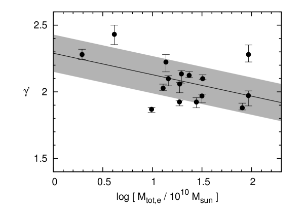
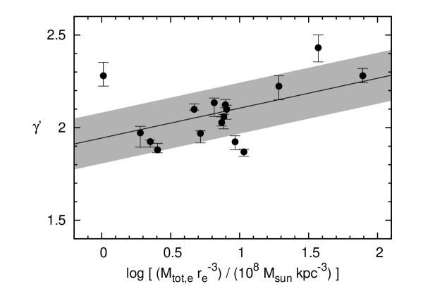
Figure 5: Logarithmic slope of the total density profile $\gamma^{\prime}$ against the total mass enclosed within the three-dimensional radius $r_{\mathrm{e}}$ (upper panel) and the average total mass density inside $r_{\mathrm{e}}$ (lower panel). The solid black line is a linear fit to the relation (including scatter), and the gray band indicates the intrinsic scatter.

There is some evidence (non-zero slope with about $2$-sigma significance) for a slight anti-correlation between the total mass $M_{\mathrm{tot,e}}$ and $\gamma^{\prime}$ (see Figure 5, upper panel, and Table 3), i.e. the total density slope tends to be steeper for the least massive systems. The most notable outlier is SDSS J0935, which, despite being the most massive galaxy in the sample, has a $\gamma^{\prime}$ comparable to that of the two systems with $M_{\mathrm{tot,e}}<10^{11}M_{\sun}$. We also find a correlation (with similar significance) between $\gamma^{\prime}$ and the quantity $\log(M_{\mathrm{tot,e}}/r_{\mathrm{e}}^{3})$, which is a proxy for the average total mass density inside the three-dimensional radius $r_{\mathrm{e}}$ (Figure 5, lower panel). This trend is in agreement with the findings of Auger et al. (2010a), who observe a relatively tight correlation between $\gamma^{\prime}$ and the central surface mass density of the full SLACS sample.

We note that the covariance between $\gamma^{\prime}$ and $M_{\mathrm{tot,e}}$ is generally very small. In fact, for a given Einstein mass and radius, the dependence on the slope of the total mass $M_{\mathrm{tot}}(r)$ enclosed inside the three-dimensional radius $r$ is least in the region where $r/R_{\mathrm{Einst}}\simeq 2$. For most of the galaxies in our sample, the ratio $R_{\mathrm{e}}/R_{\mathrm{Einst}}$ is not far from that value, so that the 1-sigma uncertainty on $\gamma^{\prime}$ usually translates into a mass change of less than 1 per cent (and even in the case of J0935, which has $R_{\mathrm{e}}/R_{\mathrm{Einst}}\simeq 5$, it only reaches about 4 per cent, i.e. less than 0.02 in dex).

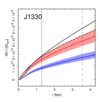
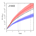
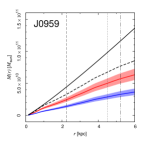
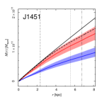
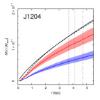
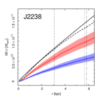
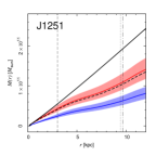
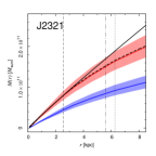
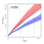
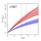
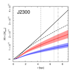
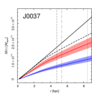
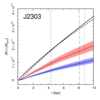
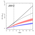
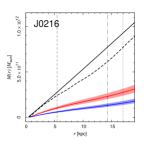
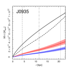
Figure 4: Compilation of spherically averaged mass distributions for the sample galaxies, sorted by increasing $M_{\mathrm{tot,e}}$. In each panel, the solid black line shows the total mass profile obtained from the best reconstructed model, and the dashed black line indicates the maximal luminous mass profile calculated under the maximum bulge (i.e. minimum halo) hypothesis (see Sect. 4.2.1). The solid red line shows the luminous mass profile rescaled using the value for stellar mass determined from SPS analysis (Auger et al., 2009), adopting a Salpeter IMF. The red-shaded region represents the corresponding uncertainty (i.e., the standard deviation of the marginalized posterior for the stellar mass). The blue curves and regions have the same meaning, but are obtained with a Chabrier IMF. The vertical lines indicate the location of the effective radius (dotted line), the Einstein radius (dashed line) and the outermost boundary of the kinematic data (dash-dotted line).

Table 2: Recovered masses, dark matter fractions and dynamical quantities for the sixteen sample SLACS lens galaxies.

Galaxy name	$\log\frac{\displaystyle M_{\mathrm{tot,e}}}{\displaystyle M_{\sun}}$	$M_{\ast}/L_{\sun,B}$	$f_{\mathrm{DM}}^{\mathrm{mb\phantom{p}}}$	${f}_{\mathrm{DM}}^{\mathrm{Chab}\phantom{p}}$	$f^{\mathrm{Salp}}_{\mathrm{DM}}$	$v/\sigma$	$j_{z}$	$\lambda_{R}$	$\delta$	$\gamma$
SDSS J0037$-$0942	11.50	4.85	0.23	$0.66^{+0.04}_{-0.05}$	$\phantom{-}0.40^{+0.08}_{-0.09}$	0.08	0.25	0.05	$\phantom{-}0.16$	$-0.37$
SDSS J0216$-$0813	11.97	9.80	0.17	$0.83^{+0.03}_{-0.03}$	$\phantom{-}0.70^{+0.04}_{-0.05}$	0.04	0.12	0.02	$\phantom{-}0.08$	$-0.17$
SDSS J0912$+$0029	11.91	9.00	0.30	$0.77^{+0.03}_{-0.04}$	$\phantom{-}0.59^{+0.06}_{-0.07}$	0.12	0.23	0.13	$\phantom{-}0.07$	$-0.15$
SDSS J0935$-$0003	11.97	7.17	0.12	$0.81^{+0.03}_{-0.03}$	$\phantom{-}0.67^{+0.05}_{-0.06}$	0.10	0.17	0.03	$\phantom{-}0.24$	$-0.64$
SDSS J0959$+$0410	10.99	7.63	0.30	$0.71^{+0.04}_{-0.05}$	$\phantom{-}0.49^{+0.07}_{-0.08}$	0.49	0.65	0.42	$-0.16$	$\phantom{-}0.27$
SDSS J1204$+$0358	11.14	7.55	0.02	$0.57^{+0.06}_{-0.08}$	$\phantom{-}0.23^{+0.10}_{-0.11}$	0.03	0.07	0.03	$\phantom{-}0.09$	$-0.19$
SDSS J1250$+$0523	11.29	3.55	0.05	$0.35^{+0.10}_{-0.11}$	$-0.14^{+0.17}_{-0.20}$	0.15	0.16	0.09	$\phantom{-}0.22$	$-0.56$
SDSS J1251$-$0208	11.27	3.56	0.46	$0.67^{+0.05}_{-0.07}$	$\phantom{-}0.43^{+0.10}_{-0.11}$	0.82	0.81	0.66	$-0.36$	$\phantom{-}0.53$
SDSS J1330$-$0148	10.29	5.55	0.05	$0.51^{+0.06}_{-0.07}$	$\phantom{-}0.15^{+0.11}_{-0.12}$	0.52	0.49	0.48	$-0.05$	$\phantom{-}0.09$
SDSS J1443$+$0304	10.62	4.04	0.01	$0.32^{+0.09}_{-0.10}$	$-0.20^{+0.16}_{-0.18}$	0.36	0.60	0.37	$\phantom{-}0.13$	$-0.30$
SDSS J1451$-$0239	11.11	4.04	0.12	$0.51^{+0.07}_{-0.09}$	$\phantom{-}0.19^{+0.10}_{-0.12}$	0.10	0.31	0.05	$\phantom{-}0.15$	$-0.35$
SDSS J1627$-$0053	11.37	4.85	0.21	$0.50^{+0.09}_{-0.11}$	$\phantom{-}0.12^{+0.16}_{-0.20}$	0.07	0.18	0.06	$\phantom{-}0.16$	$-0.38$
SDSS J2238$-$0754	11.16	5.91	0.08	$0.62^{+0.05}_{-0.06}$	$\phantom{-}0.33^{+0.09}_{-0.10}$	0.43	0.66	0.42	$-0.18$	$\phantom{-}0.30$
SDSS J2300$+$0022	11.44	7.22	0.23	$0.69^{+0.05}_{-0.05}$	$\phantom{-}0.45^{+0.08}_{-0.10}$	0.03	0.15	0.02	$\phantom{-}0.08$	$-0.17$
SDSS J2303$+$1422	11.51	7.48	0.04	$0.69^{+0.04}_{-0.05}$	$\phantom{-}0.46^{+0.07}_{-0.08}$	0.05	0.19	0.04	$\phantom{-}0.14$	$-0.31$
SDSS J2321$-$0939	11.27	4.81	0.12	$0.51^{+0.08}_{-0.10}$	$\phantom{-}0.13^{+0.15}_{-0.18}$	0.06	0.08	0.06	$\phantom{-}0.15$	$-0.36$

Note. For each galaxy we list: the logarithm of the total mass $M_{\mathrm{tot,e}}$ enclosed within the three-dimensional radius $r_{\mathrm{e}}$; the stellar mass-to-light ratio (in the $B$-band) corresponding to the maximal luminous profile; the fraction of dark over total mass within $r_{\mathrm{e}}$ for the maximum bulge assumption ($f_{\mathrm{DM}}^{\mathrm{mb\phantom{p}}}$) and for the Chabrier and Salpeter IMFs (${f}_{\mathrm{DM}}^{\mathrm{Chab}\phantom{p}}$ and $f^{\mathrm{Salp}}_{\mathrm{DM}}$, respectively); the inclination-corrected $v/\sigma$ ratio; the dimensionless angular momentum $j_{z}$; the Emsellem kinematic parameter $\lambda_{R}$; the global anisotropy parameters $\delta$ and $\gamma$.

4.2 Luminous mass and dark matter content

The radial profile for the luminous component is obtained from the best reconstructed stellar DF. However, since the adopted modelling approach treats the stellar distribution as a tracer embedded in the total potential, the normalization of the luminous profile remains unconstrained, and further assumptions (§ 4.2.1) or additional information (§ 4.2.2) are therefore necessary to set its scale and determine the contribution of the dark matter component at different radii.

4.2.1 Dark matter fraction: constraints from the maximum bulge approach

When additional information on the normalization is unavailable, the most straightforward approach consists in maximally rescaling the luminous profile under the physical constraint that it does not exceed the total mass distribution at any point, and the assumption that the stellar mass-to-light ratio is fairly position-independent. This procedure is known as the minimum halo or maximum bulge hypothesis, and is the analogue for early-type galaxies of the classical maximum disk hypothesis (van Albada & Sancisi, 1986) routinely adopted in the study of late-type galaxies. It is frequently employed (see e.g. Barnabè et al. 2009a and Weijmans et al. 2009 for recent applications) since it provides a consistent and robust method to determine a conservative lower limit for the dark matter fraction in the galaxy, within the considered region.

The (spherically averaged) luminous mass profiles obtained under the maximum bulge hypothesis are presented as dashed black lines in Figure 4. Let $M_{\mathrm{\ast,e}}^{\mathrm{mb}}$ denote the corresponding stellar mass enclosed inside the spherical radius $r_{\mathrm{e}}$. We see that the lower limit for the (three-dimensional) fraction of dark over total mass within that radius, defined as $f_{\mathrm{DM}}\equiv 1-M_{\mathrm{\ast,e}}^{\mathrm{mb}}/M_{\mathrm{tot,e}}$, varies very significantly from system to system (cf. Table 2): three of the galaxies, SDSS J1443, SDSS J1204 and SDSS J2303, show a dark matter lower limit $f_{\mathrm{DM}}<5$ per cent within the probed region, whereas — on the opposite end — several galaxies require at least one fifth of the total mass enclosed within $r_{\mathrm{e}}$ to be dark, with a peak of 46 per cent for SDSS J1251. The average and median of the dark matter fraction lower limits for the sample, obtained under the maximum bulge approach, are, respectively, $f_{\mathrm{DM}}=16$ and $12$ per cent.

The stellar mass-to-light ratios (in the $B$-band) corresponding to the maximal luminous profiles are in the range $3<M_{\ast}/L_{\sun,B}<10$, fully consistent with the values determined for local early-type galaxies (see e.g. Kronawitter et al. 2000 Gerhard et al. 2001, Trujillo, Burkert, & Bell 2004, Mamon & Łokas 2005). However, when taking into account passive stellar evolution, galaxies at higher redshift are expected to have smaller $M_{\ast}/L_{\sun,B}$ than their local counterparts (an effect that becomes significant already at $z\gtrsim 0.1$, see Treu et al. 2002).

4.2.2 Dark matter fraction: constraints from stellar mass estimates

While calculating a lower limit for the dark matter content is useful, galaxies need not have maximal bulges. We therefore set the scale for the luminous mass profiles by adopting, for each system, the stellar mass inferred from stellar population synthesis models, assuming either a Chabrier (2003) or a Salpeter (1955) IMF. We use stellar mass values taken from the stellar population analysis performed by Auger et al. (2009) on a data set constituted by deep, high-resolution, multi-band HST observations of the SLACS lenses.

The spherically averaged luminous mass profiles obtained in this way are presented in Figure 4. Figure 6 shows the corresponding dark matter fractions within $r_{\mathrm{e}}$, following the definition for $f_{\mathrm{DM}}$ given above in § 4.2.1 and replacing $M_{\mathrm{\ast,e}}^{\mathrm{mb}}$ with the stellar masses $M_{\mathrm{\ast,e}}^{\,\mathrm{Chab}}$ and $M_{\mathrm{\ast,e}}^{\mathrm{Salp}}$ for Chabrier and Salpeter IMFs, respectively.

We find that, independently of the specific choice of the IMF, there is a significant correlation (greater than 3-sigma) between the dark matter fraction within $r_{\mathrm{e}}$ and the total mass (the parameters of the fit are given in Table 3). Such a correlation was first observed, in the SLACS sample, by Auger et al. (2010a). Their result is confirmed and strengthened by the present study, where we conduct a more rigorous and detailed joint analysis on a sub-sample of SLACS galaxies, taking advantage of the extended kinematic information (rather than an estimate of the stellar velocity dispersion $\sigma_{\mathrm{SDSS}}$ within a single 3 arcsec diameter aperture), and self-consistently including axial symmetry and stellar anisotropy in the model, and we reach analogous conclusions.

The normalization based on the stellar masses inferred from Salpeter IMF produces a luminous profile that, when compared to Chabrier, is always closer to the one determined under the maximum bulge assumption, and in several cases is fully consistent with it. For two systems, SDSS J1250 and in particular SDSS J1443, this luminous profile (including the error band) locally exceeds the maximum bulge curve, indicating that it unphysically overshoots the total mass in places, thus producing the two negative $f_{\mathrm{DM}}$ points in Figure 6. Taken at face value, this would lead to the conclusion that the Salpeter relation constitutes an inadequate IMF for these two galaxies (and therefore must be rejected for all systems if we assume the IMF to be universal), whereas the Chabrier IMF — which gives lower stellar masses by almost a factor of 2 — never fails to produce physical results. However, it must be noted that in both cases the lower limit of the error band is only slightly higher ($\lesssim 5$ per cent) than the maximal luminous curve, and the adopted uncertainties represent 1-$\sigma$ errors (see Auger et al. 2009 for the details of how these uncertainties are calculated within a Bayesian framework). Moreover, several systematic effects (such as the circularization of the profile and the discreteness of the TIC building blocks used to construct the model galaxy) might interfere at the few per cent level with the minute details of the reconstructed luminous profile. Therefore, we conservatively conclude that all the analyzed systems are consistent with having stellar masses determined from a Salpeter-like IMF.

With a Salpeter IMF, the recovered dark matter fraction for systems having total masses $\log(M_{\mathrm{tot,e}}/M_{\sun})\lesssim 11.5$ spans from 0 to $\sim 50$ per cent, whereas the three most massive galaxies are already dominated by dark matter ($f_{\mathrm{DM}}$ is approximately 60 to 70 per cent) inside 1 $r_{\mathrm{e}}$. The average and median dark matter fractions are, respectively, $f^{\mathrm{Salp}}_{\mathrm{DM}}=31$ and $37$ per cent. The importance of the dark component becomes even more extreme if a Chabrier IMF is considered (average $f^{\mathrm{Chab}}_{\mathrm{DM}}=61$ per cent, median $f^{\mathrm{Chab}}_{\mathrm{DM}}=64$ per cent), with the luminous component contributing less than 50 per cent to $M_{\mathrm{tot,e}}$ in all systems but two.

It has been suggested that the IMF is not universal but becomes systematically ‘heavier’ for more massive galaxies (see Treu et al. 2009, Auger et al. 2010b, van Dokkum & Conroy 2010, Thomas et al. 2011; but see also Napolitano, Romanowsky, & Tortora 2010 for a different conclusion). The data presented here are consistent with this fact and cannot resolve the degeneracy between varying IMF and varying dark matter fraction, as we discuss in Section 6.

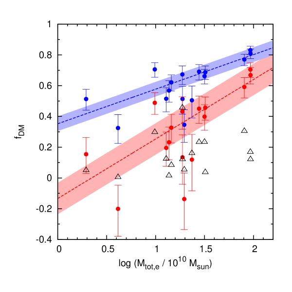
Figure 6: Dark matter fractions versus the total mass enclosed within the three-dimensional radius $r_{\mathrm{e}}$. The upwards black triangles indicate the dark matter fraction lower limits calculated from the maximum bulge approach. The full circles show the dark matter fractions obtained when luminous masses are determined via SPS analysis, assuming Salpeter (red) or Chabrier (blue) IMFs. The dashed lines are linear fits to the relation, calculated including intrinsic scatter (which is indicated by the coloured bands).

Table 3: Summary of linear relations derived for the SLACS lenses.

X	Y	Slope	Intercept	Scatter
$\log(M_{\mathrm{tot,e}})$	$\gamma^{\prime}$	$-0.16\pm 0.09$	$\phantom{-}2.29\pm 0.13$	$0.14^{+0.06}_{-0.01}$
$\log(M_{\mathrm{tot,e}}/r_{\mathrm{e}}^{3})$	$\gamma^{\prime}$	$\phantom{-}0.16\pm 0.09$	$\phantom{-}1.94\pm 0.08$	$0.14^{+0.06}_{-0.01}$
$\log(M_{\mathrm{tot,e}})$	${f}_{\mathrm{DM}}^{\mathrm{Chab}}$	$\phantom{-}0.22\pm 0.04$	$\phantom{-}0.35\pm 0.06$	$0.05^{+0.04}_{-0.03}$
$\log(M_{\mathrm{tot,e}})$	${f}_{\mathrm{DM}}^{\mathrm{Salp}}$	$\phantom{-}0.39\pm 0.08$	$-0.13\pm 0.12$	$0.10^{+0.06}_{-0.04}$

Note. The mass $M_{\mathrm{tot,e}}$ is in units of $10^{10}M_{\sun}$, while the density $M_{\mathrm{tot,e}}/r_{\mathrm{e}}^{3}$ is in units of $10^{8}M_{\sun}$ kpc^-3.

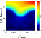
(a) J1204

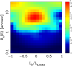
(b) J2321

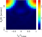
(c) J0216

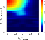
(d) J1250

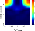
(e) J2300

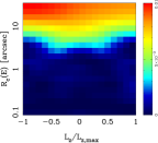
(f) J0935

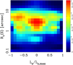
(g) J1627

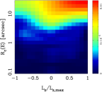
(h) J2303

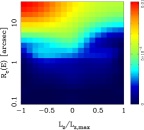
(i) J0912

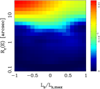
(j) J0037

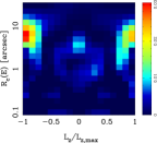
(k) J1451

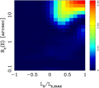
(l) J1330

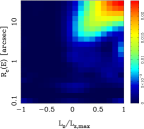
(m) J1443

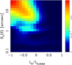
(n) J0959

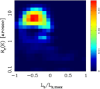
(o) J2238

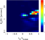
(p) J1251

Figure 7: Best model reconstruction of the weighted two-integral DFs of the sample galaxies. The value of each pixel represents the relative contribution of the corresponding TIC to the luminous mass of the galaxy. The galaxies are sorted by increasing values of the specific angular momentum parameter $j_{z}$.

5 Dynamical structure

A major strength of the method described in Sect. 3 is that the cauldron algorithm also provides, for each analyzed galaxy, the associated (weighted) two-integral stellar DF, which constitutes the most general and complete description of the dynamical structure of the system within the context of the adopted model. The DF can equivalently be represented as a bi-dimensional map of the TIC weights in the integral space $(E,L_{z})$: the value of each pixel simply indicates the relative stellar-mass contribution due to the TIC building block of corresponding energy and angular momentum.

Figure 7 shows the maps of the TIC weights that are obtained for the best-reconstructed model (i.e., the MAP model) of each lens galaxy. In keeping with the analysis of SDSS J0728 (Barnabè et al., 2010), the most recent study of a lens galaxy performed with cauldron, we make use of a library composed of 360 TICS: for each one of the $N_{E}=20$ elements logarithmically sampled in the circular radius $R_{\rm c}$ (corresponding to a grid in energy, see Barnabè & Koopmans 2007) we consider $N_{L_{z}}=9$ elements linearly sampled in the normalized angular momentum $0\leq L_{z}/L_{z,\mathrm{max}}\leq 1$, and the mirrored negative $L_{z}/L_{z,\mathrm{max}}$ values. Although a grid of $(N_{E}=10)\times(N_{L_{z}}=5)$ has been shown to be generally sufficient to provide a satisfactory reconstruction of the observables (Barnabè et al., 2009a), a finer grid does a better job in reducing the undesired discreteness effect of the TIC superposition (e.g. on the surface brightness, kinematic and local $\langle v_{\varphi}\rangle/\bar{\sigma}$ maps).

The DF encapsulates the description of the stellar component of the galaxy in an very compact way, which can not be straightforwardly decoded at a glance. Therefore, we now proceed to distill much of that information into more directly interpreted quantities of astrophysical interest that characterize the dynamical status of the system on a global and local level, i.e. the ratio between ordered and random motions, the specific angular momentum and the global anisotropy of the stellar velocity dispersion tensor.

5.1 Global and local $v/\sigma$

Figure 8 shows the location of the sixteen analyzed lens galaxies on the model version of the classical $(v/\sigma,\epsilon)$ diagram. The quantity $v/\sigma$ is commonly used as a global indicator of the importance of ordered motions (i.e. rotation) with respect to random motions in a stellar system. For each galaxy we calculate the ratio $v/\sigma$, corrected to an edge-on view, from the two-dimensional kinematic maps of the best reconstructed model, following the prescriptions of Binney (2005) for extended kinematic data sets. The ratio is plotted against the inclination-corrected ellipticity of the light distribution $\epsilon_{\ast}\equiv 1-q_{\ast}$, where $q_{\ast}$ is the axial ratio introduced in Sect. 3.4.2.

We find that the dynamics of most systems is clearly dominated by random motions, with $v/\sigma\leq 0.15$, while rotation plays a significant role in the remaining five galaxies. The members of the latter group have several common characteristics, beyond being above a $v/\sigma$ ratio of 0.35: (i) they are all fast rotators, according to both the definition of Emsellem et al. (2007) and their specific angular momentum content (as discussed below in Sect. 5.2); (ii) they are quite flattened in the light (having $0.38<q_{\ast}<0.74$); (iii) they belong to the lower half of the sample in terms of $M_{\mathrm{tot,e}}$, including, moreover, the three least massive galaxies of the whole sample (namely, SDSS J1330, SDSS J1443 and SDSS 0959).

As a comparison to the SLACS systems, Figure 8 also displays the location on the diagram of a sub-sample of 24 SAURON early-type galaxies, whose observables have also been corrected for inclination, analyzed by Cappellari et al. (2007). The two samples generally occupy similar positions in the $(v/\sigma,\epsilon)$ space, although the SLACS galaxies lack the most extreme cases (such as the very flattened slow rotator NGC 4550 and the fast rotator NGC 3156 with a $v/\sigma\sim 1$) and show a sharper transition between dispersion- and rotation-dominated systems. This, however, is likely a consequence of the limited number of fast rotating galaxies present among the SLACS sample, mainly comprised of massive systems ($\sigma_{\mathrm{SDSS}}\gtrsim 200$ km s^-1) which tend to be slow rotators.

From the stellar DF it is also possible to derive a description of the intrinsic kinematics of the galaxy by using the internal velocity moments to define — at each point $(R,z)$ in the meridional plane — the quantity $\langle v_{\varphi}\rangle/\bar{\sigma}$, where $\langle v_{\varphi}\rangle$ is the local mean azimuthal velocity (i.e. around the symmetry axis) and $\bar{\sigma}^{2}\equiv(\sigma_{R}^{2}+\sigma_{\varphi}^{2}+\sigma_{z}^{2})/3$ is the mean velocity dispersion. This ratio can be interpreted as a local and intrinsic analogue of the global indicator $v/\sigma$, since it characterizes the importance of rotation with respect to random motions at each position inside the galaxy. Figure 9 shows the $\langle v_{\varphi}\rangle/\bar{\sigma}$ maps for all the sample galaxies, extending up to $r_{\mathrm{e}}/2$ and sorted by increasing specific angular momentum $j_{z}$ (see Sect. 5.2). For visualization purposes, and in particular to make the comparison among fast rotators easier, the maps are presented as having the same sense of rotation (where applicable).

By examining the $\langle v_{\varphi}\rangle/\bar{\sigma}$ maps, the sample galaxies clearly fall into two broad groups on the basis of their dynamical status. The first 11 systems are overall dominated by random motions; in a few systems, such as SDSS J0935 and SDSS J1451, islands of moderate rotation ($|\langle v_{\varphi}\rangle|/\bar{\sigma}\approx 0.5$) are present, but remain confined to small, spatially limited regions. What sets apart the remaining five galaxies, on the other hand, is the presence of strong rotation on a large scale pattern. This structural difference reflects the classification of the two groups as, respectively, slow and fast rotators. Guided by the intuition provided by these maps, in the next Section we provide a more quantitative criterion, based on the angular momentum content, to specify to which one of the two groups the modelled galaxies belong.

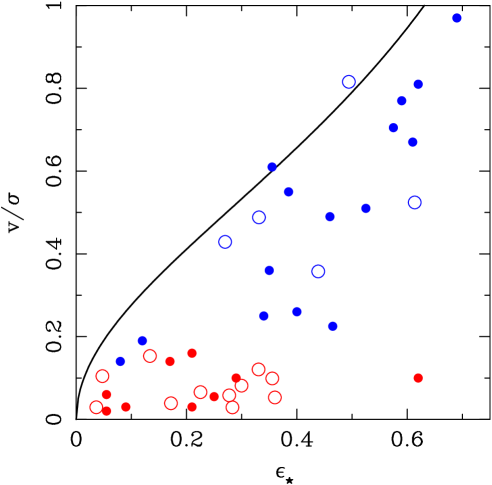
Figure 8: Model $(v/\sigma,\epsilon)$ diagram for the sixteen lens galaxies in our sample (open circles), divided in fast and slow rotators (blue and red points, respectively); $\epsilon_{\ast}$ is the intrinsic ellipticity of luminous distribution, and $v/\sigma$ is calculated from the best model, corrected to an edge-on inclination. As a comparison, the plot also shows, as full circles, the corresponding quantities (also corrected for inclination) for the 24 nearby SAURON ellipticals studied in Cappellari et al. (2007). The solid line represents the location of edge-on isotropic rotators (assuming $\alpha=0.15$, see Binney 2005).

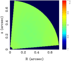
(a) J1204

(b) J2321

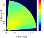
(c) J0216

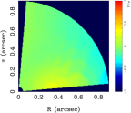
(d) J1250

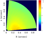
(e) J2300

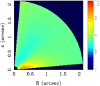
(f) J0935

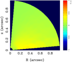
(g) J1627

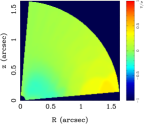
(h) J2303

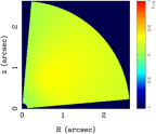
(i) J0912

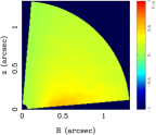
(j) J0037

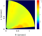
(k) J1451

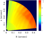
(l) J1330

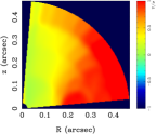
(m) J1443

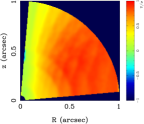
(n) J0959

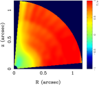
(o) J2238

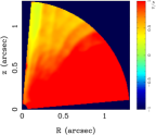
(p) J1251

Figure 9: Maps of the local $\langle v_{\varphi}\rangle/\bar{\sigma}$ ratio between the mean rotation velocity around the $z$-axis and the mean velocity dispersion, plotted up to $R_{\mathrm{e}}/2$ in the positive quadrant of the meridional plane. As in Fig. 7, the galaxies are sorted by increasing $j_{z}$.

5.2 The angular momentum of slow and fast rotators

We recall the definition of the dimensionless specific angular momentum of the stellar component $j_{z}$ (see Barnabè et al., 2009a):

$$j_{z}\equiv\frac{\displaystyle\int\rho_{\ast}R\,|\langle v_{\varphi}\rangle|\,\mathrm{d}^{3}\mn@boldsymbol{x}}{\displaystyle\int\rho_{\ast}R\sqrt{{\langle v_{\varphi}\rangle}^{2}+\bar{\sigma}^{2}}\,\mathrm{d}^{3}\mn@boldsymbol{x}}\,,$$ (9)

where $\rho_{\ast}=\int f\,\mathrm{d}^{3}\mn@boldsymbol{v}$ is the density of the luminous component obtained from the MAP model stellar DF $f$. For each galaxy in the sample, we carry out this integral up to $r_{\mathrm{e}}/2$, tabulating the results in Table 2. We find that the galaxies can be neatly divided in two groups depending on the value of the quantity $j_{z}$: on one side 11 low angular momentum systems, with $j_{z}\lesssim 0.3$, and on the other side five objects with $j_{z}\simeq 0.5$ or greater. By comparing with the local $\langle v_{\varphi}\rangle/\bar{\sigma}$ maps, we see that these five systems are also the only ones that clearly exhibit large scale rotation. Therefore, we choose to classify the galaxies on the basis of their specific angular momentum content by labelling as slow and fast rotators the systems that are, respectively, below and above $j_{z}=0.4$.

In Figure 10 we plot, for each system, $j_{z}$ versus the quantities $v/\sigma$ (inclination-corrected, Sect. 5.1) and $\lambda_{R}$, computed on the kinematic data set of the best reconstructed model. The observational parameter $\lambda_{R}$ was first introduced by Emsellem et al. (2007) as a consistent way to quantify the specific stellar angular momentum (in projection) of an early-type galaxy for which two-dimensional kinematic maps are available, and its value is employed as the criterion to discriminate between slow ($\lambda_{R}<0.1$) and fast ($\lambda_{R}>0.1$) rotating systems. The model quantity $j_{z}$ is, by construction, the three-dimensional and intrinsic analogue of $\lambda_{R}$. Figure 10 shows that classifying the rotators on the basis of either of these two parameters yields fully equivalent results for all galaxies but one, SDSS J0912. We have already singled out this system (in Sect. 4) as the only one for which the kinematic maps do not reach half of the effective radius. The misclassification of SDSS J0912 can be ascribed to the spatially limited data set, since slow rotators commonly show decreasing $\lambda_{R}$ profiles for $R/R_{\mathrm{e}}\lesssim 0.5$, and thus the parameter can exceed the threshold value of 0.1 in the inner regions (see Emsellem et al. 2007 and in particular their Figure 2).

It is worth noting that, for slow rotators, the spread in $\lambda_{R}$ is much smaller than the spread in $j_{z}$, indicating that the latter constitutes a better discriminator of the intrinsic properties of these systems.

5.3 Global velocity dispersion tensor

The global stellar velocity dispersion tensor constitutes a useful and concise characterization of the overall dynamical structure of a stellar system. It is customary to describe its shape by means of the three global anisotropy parameters (Cappellari et al., 2007; Binney & Tremaine, 2008)

$$\beta\equiv 1-\frac{\Pi_{zz}}{\Pi_{RR}},\quad\gamma\equiv 1-\frac{\Pi_{\varphi\varphi}}{\Pi_{RR}}\quad\textrm{and}\quad\delta\equiv 1-\frac{2\Pi_{zz}}{\Pi_{RR}+\Pi_{\varphi\varphi}},$$ (10)

where we denote the total unordered kinetic energy along the coordinate direction $k$ as

$$\Pi_{kk}=\int\rho_{\ast}\sigma^{2}_{k}\,\mathrm{d}^{3}\mn@boldsymbol{x}\,,$$ (11)

and $\sigma^{2}_{k}(\mn@boldsymbol{x})\equiv\langle v^{2}_{k}\rangle-{\langle v_{k}\rangle}^{2}$ is the local stellar velocity dispersion in the $k$ direction. For a fully isotropic object the values of all three parameters become zero. If the galaxy is only isotropic in the meridional plane, then $\beta=0$ and the remaining parameters are related by $\gamma=2\delta/(\delta-1)$. The latter scenario is the one that applies to the galaxy models considered in this analysis, since, for any axisymmetric collisionless system supported by a two-integral DF, $\langle v^{2}_{R}\rangle=\langle v^{2}_{z}\rangle$ everywhere, the meridional velocities $\langle v_{R}\rangle$ and $\langle v_{z}\rangle$ are null, and therefore $\Pi_{RR}=\Pi_{zz}$.

The values of the global parameters $\delta$ and $\gamma$ for the SLACS galaxies, calculated within $r_{\mathrm{e}}/2$, are reported in Table 2. The slow rotators are all mildly anisotropic, quite similarly to what is found for their nearby counterparts (Cappellari et al., 2007): the values of $\delta$ fall between 0.05 and 0.25, and $\delta\lesssim 0.15$ for most systems. The fast rotating galaxies, with the exception of SDSS J1443, exhibit instead negative $\delta$ values. This is a consequence of the adopted dynamical model: due to the isotropy in the meridional plane, it follows from Eq. (10) that every system for which $\sigma^{2}_{\varphi}<\sigma^{2}_{R}$ over most of the luminosity density-weighted volume (so that $\Pi_{\varphi\varphi}<\Pi_{RR}$) is characterized by $\delta<0$, i.e. is anisotropic in the sense of having a smaller pressure along the equatorial plane than perpendicular to it. Moreover — within the approach of modelling based on TIC superposition — very fast rotating systems tend to have small azimuthal velocity dispersions $\sigma^{2}_{\varphi}$, since their dynamical description is dominated by co-rotating TIC building blocks of similar angular momentum. This can be more easily illustrated by considering the limiting case of a hypothetical system described by a single TIC: for this simple object one has $\langle v^{2}_{\varphi}\rangle={\langle v_{\varphi}\rangle}^{2}$, and thus $\sigma^{2}_{\varphi}=0$, everywhere in the meridional plane within the zero-velocity curve, so that $\delta_{\mathrm{TIC}}=-1$ and $\gamma_{\mathrm{TIC}}=1$. It is not surprising, therefore, that the three fastest rotating galaxies in the sample (SDSS J0959, SDSS J2238 and SDSS J1251) are all found to have clearly negative values of $\delta$.

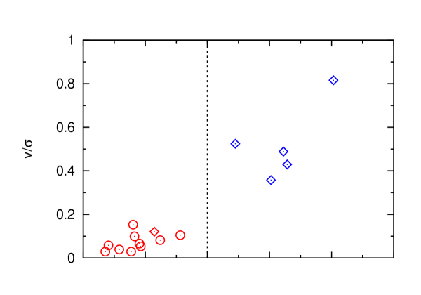
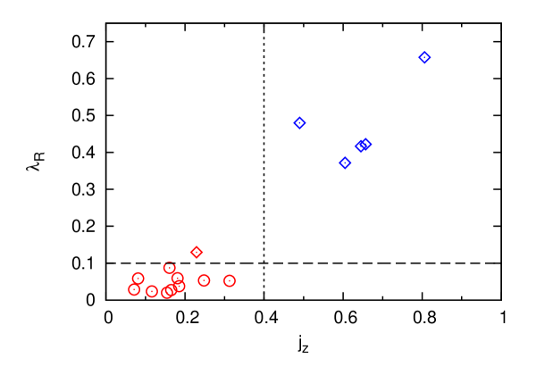
Figure 10: The intrinsic dynamical parameter $j_{z}$ versus the inclination-corrected $v/\sigma$ ratio (top panel) and the Emsellem kinematic parameter $\lambda_{R}$ (bottom panel) for the sixteen SLACS lens galaxies in the sample. The circles and diamonds indicate, respectively, the slow and fast rotating systems classified according to the Emsellem et al. (2007) definition of the threshold value that divides the two types, i.e. $\lambda_{R}=0.1$ (horizontal dashed line). The red and blue symbols denote the slow and fast rotators when the galaxies are classified on the basis of the dimensionless angular momentum (threshold value $j_{z}=0.4$, vertical dotted line). The two classifications produce fully equivalent results for all systems barring SDSS J0912 (indicated with the red diamond), which is the galaxy with the most spatially limited kinematic maps (see text).

6 Discussion

The study presented in this paper represents the most detailed analysis conducted so far of the total mass density profile of a relatively large sample of E/S0 galaxies beyond the local Universe, making consistent use of axially symmetric density distributions for both the lensing and dynamical modelling, and taking advantage of the constraints provided by two-dimensional kinematic information.

6.1 Total density profile

The results of this work corroborate the mounting evidence (see Sect. 1) that the inner regions (on the scale of the effective radius) of massive early-type galaxies are characterized by an approximately isothermal total density distribution (i.e., $\rho_{\mathrm{tot}}\propto r^{-\gamma^{\prime}}$, with $\gamma^{\prime}\approx 2$), a property often referred to as the ‘bulge–halo conspiracy’. This name owes to the fact that there appears to be no obvious physical explanation of why the luminous and dark matter components of each system, despite not obeying a power-law distribution, should often ‘conspire’ to produce a nearly $1/r^{2}$ total profile.

By examining individual lens galaxies in great detail, however, we can conclude that the purported conspiracy only holds in first approximation: even though we provide confirmation that all systems, quite remarkably, can be effectively modelled by a simple and smooth single power-law profile for $\rho_{\mathrm{tot}}$, the average logarithmic slope is found to be $\langle\gamma^{\prime}\rangle=2.074^{+0.043}_{-0.041}$, i.e. slightly (but significantly) super-isothermal. Moreover, and perhaps more importantly, different galaxies do exhibit noticeably different slopes, with an intrinsic scatter in $\langle\gamma^{\prime}\rangle$ of about 7 per cent. These results are in agreement with the findings of Koopmans et al. (2009) and Auger et al. (2010a) for the full sample of SLACS lenses, obtained by making use of spherical Jeans models for the dynamics, constrained by a single kinematic measurement, i.e. the stellar velocity dispersion $\sigma_{\mathrm{SDSS}}$ inside the 3 arcsec diameter SDSS fiber. This indicates that the combined lensing and dynamics approach is a generally robust method to determine the total density distribution of a sample of lens galaxies, even when a very simple (and not fully consistent) dynamical model is employed. The values of the logarithmic slope obtained for individual systems with the two methods — that we denote here as $\gamma^{\prime}_{\mathrm{2I}}$ and $\gamma^{\prime}_{\mathrm{Jeans}}$ — can differ by up to about 10-15 per cent, as illustrated in Figure 11. This discrepancy is typically of the order of the 1-$\sigma$ errors in $\gamma^{\prime}_{\mathrm{Jeans}}$ but, in most cases, much larger than the few per cent uncertainties on $\gamma^{\prime}$ obtained with this study, stressing the importance of having access to two-dimensional kinematic data sets and more sophisticated dynamical models when a precise measurement of a lens galaxy density profile is called for. It is interesting to note that another joint lensing and dynamics study conducted by Ruff et al. (2011) on a different sample of 11 massive early-type galaxies from the Strong Lenses in the Legacy Survey (SL2S) at a higher redshift (median $z_{\mathrm{lens}}=0.5$) also finds an average slope and an intrinsic scatter consistent with the results presented here.

Figure 11: Comparison between the total density logarithmic slope $\gamma^{\prime}_{\mathrm{2I}}$ of the sample lens galaxies obtained from the analysis conducted in this paper, making use of two-integral dynamical models and VLT VIMOS integral field spectroscopy, and the slope $\gamma^{\prime}_{\mathrm{Jeans}}$ derived by Auger et al. (2010a), using spherical Jeans models and a single kinematic measurement. Red and blue points denote, respectively, slow and fast rotators. The dashed line traces the one-to-one relationship. For both $\gamma^{\prime}_{\mathrm{2I}}$ and $\gamma^{\prime}_{\mathrm{Jeans}}$, the uncertainties represent the 68 per cent confidence interval. The slope of galaxy SDSS 1251 is not listed, as it was not included in the Auger et al. (2010a) sample of early-type systems.

It has been well established by N-body cosmological simulations that dissipationless processes produce inner density distributions with logarithmic slopes $\gamma^{\prime}\approx 1$ (e.g. Navarro et al., 1996) or even shallower (e.g. Graham et al., 2006; Navarro et al., 2010). Moreover, subsequent dissipationless merging (i.e., dry merging) preserves the steepness of the inner density profile (Dehnen, 2005; Kazantzidis et al., 2006). It follows, therefore, that the interplay between dark matter and the baryonic component, with its complex dissipative processes, plays a key role and must be taken into account in order to explain the emergence of the isothermal profile in the inner regions of galaxies. Numerical work (see e.g. Gnedin et al. 2004, Abadi et al. 2010 and references therein) on the response of dark matter to the condensation of baryons does indeed show that the assembly of a central galaxy makes the halo significantly more concentrated, producing a steeper total density slope. The high-resolution simulations of moderately massive systems (with halo masses comparable to that of the Milky Way) carried out by Tissera et al. (2010), which include a detailed treatment of baryonic processes, reveal a nearly isothermal profile over a relatively large radial range extending up to the baryonic radius (defined as the radius containing 83 per cent of the stellar and gaseous component of the galaxy, i.e. the region within which the baryons play an important role). Aside from this general global result, however, the details of the density distribution are largely determined by the specific assembly history of each system. This suggests that the observed scatter in the $\gamma^{\prime}$ values of the SLACS lenses is a consequence of the idiosyncratic formation histories of the individual galaxies, and can potentially provide information on the processes involved in their build-up. Once the isothermal structure is in place, dissipationless mergers — both major and minor — preserve it not only in the inner regions, but throughout the systems (Nipoti, Treu, & Bolton, 2009). We stress, however, that, even in the case of a nearly perfectly $1/r^{2}$ seed distribution, this process produces a non-negligible scatter of about 10 per cent in the logarithmic slope (i.e. comparable to the observed level), which overlaps with the scatter that, potentially, might have been present in the parent (pre- dry mergers) density distribution, further complicating the task of reconstructing the galaxy formation history.

6.2 Mass and dynamical structure

Another defining property of early-type galaxies that we have aimed to quantify in this study is the fractional amount of dark matter that is present in the systems’ central regions. If the assumption of a constant stellar mass-to-light ratio holds, at least within the inner $R_{\mathrm{e}}$ or so, then most of the analyzed systems do require a non-negligible fraction of dark matter ($f_{\mathrm{DM}}$ greater than 10 per cent) even when the contribution of the luminous component is maximized ad hoc, without any concerns for the plausibility of the $M_{\ast}/L_{\sun,B}$ ratios involved in the rescaling. In other words, what is shown by this ‘maximum bulge’ approach is that the mass-follows-light hypothesis is necessarily violated in the majority of cases.

Adopting a physically motivated rescaling of the luminous profile — based on the stellar masses inferred from SPS models — leads to interesting results.

First of all, in agreement with previous work on the SLACS lenses (Koopmans et al., 2006; Bolton et al., 2008b; Auger et al., 2010a; Barnabè et al., 2010), we find a significant amount of dark matter within the galaxy inner regions: in the case of a Salpeter IMF, the average $f_{\mathrm{DM}}$ is 31 per cent, with a wide variation within individual objects, ranging from galaxies consistent with having no dark matter, to systems where the baryonic component accounts for less than half of the total mass already at $r_{\mathrm{e}}$. These values are broadly consistent with the results of earlier dynamical studies of nearby early-type galaxies employing a variety of different techniques and assumptions (Gerhard et al., 2001; Cappellari et al., 2006; Thomas et al., 2007; Weijmans et al., 2008; Tortora et al., 2009), which find dark matter fractions inside one half-light radius varying from 0 to about 50 per cent of the total mass, with a typical average value close to 30 per cent. If we prescribe, instead, an IMF lighter than Salpeter — as advocated for example by Cappellari et al. 2006 based on their analysis of the SAURON ellipticals, which have lower velocity dispersions than the SLACS lenses considered here — then the dark component becomes the dominant one in the central regions for almost all systems (average $f_{\mathrm{DM}}$ is $61$ per cent with a Chabrier IMF), in striking contrast with the traditional picture of early-type galaxies. It is worth noting that similarly abundant dark matter contents within the galaxy inner regions are commonly found by studies of E/S0 galaxies that adopt a Chabrier-like IMF: Grillo (2010), e.g., calculates a median value of 64 per cent (in projection) within 1 $R_{\mathrm{e}}$ for a large sample of $1.7\times 10^{5}$ massive SDSS early-type galaxies. Tortora et al. (2009), applying spherical Jeans models to a homogeneous sample of 335 local E/S0 systems, derive a $f_{\mathrm{DM}}\sim 60$ per cent. Weijmans (2009) performs a sophisticated dynamical analysis of the nearby galaxy NGC 2549 using high-quality photometry and extended kinematic maps and finds, likewise, a dark matter fraction of 65 per cent within the half-light radius by adopting a Kroupa (2001) IMF.

The second relevant result is the non-negligible positive correlation between the derived dark matter fraction and the total mass enclosed within $r_{\mathrm{e}}$. This relation is in agreement with the results of the Padmanabhan et al. (2004) study of a sample of about 30,000 SDSS ellipticals, and with the findings of Tortora et al. (2009) and Graves & Faber (2010) at lower redshift. Conversely, Grillo (2010) — by determining the stellar masses from SDSS multicolor photometry and the total mass from a simple dynamical relation, under the assumption that the galaxies can be described as spherical and isothermal systems — comes to a different conclusion, i.e. that the (projected) dark matter fraction within the half-light radius remains almost constant for values of the total mass between a few $10^{10}$ and $\sim 10^{12}$ $M_{\sun}$.

If the IMF is truly universal, then the trend for $f_{\mathrm{DM}}$ implies a genuine increase of the dark matter contribution with $M_{\mathrm{tot,e}}$, and for the most massive ellipticals the stars represent a minority component, even in the central regions (cf. Sect. 4.2.2). However, an alternative explanation is possible if the IMF varies with galaxy mass from a Chabrier/Kroupa-like functional form to a Salpeter-like one (Treu et al. 2010; see also Auger et al. 2010b), or even to a steeper low-mass end slope, as argued by van Dokkum & Conroy (2010) for the most massive systems (i.e., $\sigma\gtrsim 250$ km s^-1, which would include many of the objects studied here). We note, however, that the results from the SLACS survey only imply a mass-to-light ratio that is higher than expected for a Chabrier or Kroupa IMF. The excess mass can be provided by low mass stars (as in the case of a Salpeter IMF, as advocated by, e.g., van Dokkum & Conroy 2010), or by high mass stars remnants, in the form of neutron star and black holes (Treu et al., 2010; Auger et al., 2010b).

Finally, in terms of dynamical structure, the SLACS lenses present no surprises, and are found to be very similar to their local counterparts as observed, e.g., by SAURON (Emsellem et al., 2007; Cappellari et al., 2007). More than two-thirds of the galaxies are slow-rotating objects, as a consequence of the sample being skewed towards the high velocity dispersion end. The five fast-rotators largely coincide with the low mass tail of the sample, and all of them are high angular momentum systems, with $\lambda_{R}$ well above $0.1$, and very clearly identified as such when their $\langle v_{\varphi}\rangle/\bar{\sigma}$ meridional plane maps are examined. The dark matter fraction of the fast-rotators is consistent with the general trend, and they do not appear as a different population in terms of $f_{\mathrm{DM}}$, as suggested by Cappellari et al. (2006).

There is tentative evidence that fast-rotating galaxies are systematically more flattened in the luminous distribution than in the total density profile, despite the fact that these systems — as discussed above — are among the least massive in the sample and thus likely to be the ones where the baryonic component is most important. This would then imply that these objects lie in dark haloes whose central regions are significantly rounder than the light we observe. Such a scenario appears to be in general agreement with the results of numerical simulations (e.g. Debattista et al., 2008; Abadi et al., 2010), which show that the assembly of massive high angular momentum galaxies changes the dark halo into nearly axially symmetric, slightly oblate systems over a wide radial range. The question of whether there is an actual structural difference between the dark haloes of slow and fast rotators, however, remains pending.

7 Summary

In this work we have conducted a combined, self-consistent gravitational lensing and stellar dynamics analysis of the full sample of SLACS lens systems with available VLT VIMOS integral-field spectroscopic data, employing axially symmetric dynamical models supported by two-integral DFs. This is integrated with the constraints from stellar mass estimates derived from SPS analysis of multiband HST imaging. The application of these modelling tools on this remarkable data set has enabled us to investigate in detail the properties and three-dimensional structure of the considered sample of sixteen early-type galaxies in the redshift range $z=0.08-0.35$.

This study represents an improvement over previous joint lensing and dynamics analyses (which adopt dynamical models based on Jeans equations) and constitutes, in a sense, an extension beyond the local Universe of SAURON-type studies of the inner regions of E/S0 galaxies. Although the detailed kinematic maps available for nearby systems are clearly superior to the corresponding data sets currently obtainable for objects at $z\gtrsim 0.1$, the additional information derived from gravitational lensing provides an invaluable asset for the study of distant galaxies, which allows us to put robust constraints on their mass distribution and amount of dark matter within the probed regions.

The main conclusions from this analysis are summarized as follows.

1. The total mass density distribution of all the sample galaxies is well described, within the inner regions probed by the data sets (of order one half-light radius), by an axially symmetric power-law model. The average logarithmic slope is slightly super-isothermal, with $\langle\gamma^{\prime}\rangle=2.074^{+0.043}_{-0.041}$; there is an intrinsic scatter $\sigma_{\gamma^{\prime}}=0.144^{+0.055}_{-0.014}$ (corresponding to less than 10 per cent) around this value.

2. We find that the lens galaxies have a fairly round total mass distribution: the average axial ratio is $\langle q\rangle=0.77\pm 0.04$ and — while there are significant differences between individual systems, with an intrinsic scatter of nearly 20 per cent — all objects, barring one, are rounder than $q=0.6$. Most galaxies are about as flattened in the total distribution as they are in the luminous one.

3. The lower limit for the fraction of dark over total mass within the three-dimensional radius $r_{\mathrm{e}}$ (calculated with the maximum bulge approach under the assumption of constant stellar mass-to-light ratio inside the considered region) varies significantly between individual systems from nearly zero to almost 50 per cent, with an average value $f_{\mathrm{DM}}=16$ per cent (median value: $f_{\mathrm{DM}}=12$ per cent). The $M_{\ast}/L_{\sun,B}$ ratios corresponding to these maximal light profiles range from 3 to almost 10.

4. When the normalization of the luminous profile is set using stellar mass determinations obtained from SPS models, under the assumption of a universal IMF of the Salpeter type, we derive an average dark matter fraction $f^{\mathrm{Salp}}_{\mathrm{DM}}=31$ per cent inside $r_{\mathrm{e}}$ (median value: $f^{\mathrm{Salp}}_{\mathrm{DM}}=37$ per cent). None of the analyzed galaxies has a luminous mass distribution strongly at odds with the assumption of a Salpeter IMF (the luminous profile does exceed unphysically the circularized total mass profile for two systems, but in both cases the discrepancy is just a few per cent above the 1-$\sigma$ uncertainty).

   If one adopts a Chabrier IMF the recovered dark matter fraction becomes much higher, i.e. $f^{\mathrm{Chab}}_{\mathrm{DM}}=61$ per cent (median value: $f^{\mathrm{Chab}}_{\mathrm{DM}}=64$ per cent), which would imply that the stars represent a minority mass component even in the inner regions of early-type galaxies.

5. If the stellar masses are determined in this way, i.e. assuming a universal IMF, then the derived $f_{\mathrm{DM}}$ shows a clear correlation (3-sigma) with $M_{\mathrm{tot,e}}$, in the sense that the dark matter contribution increases with the total mass of the galaxy, becoming — even in the case of Salpeter IMF — the dominant component within $r_{\mathrm{e}}$ for the most massive ellipticals (i.e. the systems with $\log[M_{\mathrm{tot,e}}/M_{\sun}]\gtrsim 11.5$). If the IMF is not universal, than a progressive steepening of its profile with the galaxy total mass could explain, at least partially, the observed trend.

6. The SLACS lenses can be divided into two dynamically distinct groups based on the value of their specific angular momentum parameter $j_{z}$ (which we can introduce based on our three-dimensional models): about two-thirds of the galaxies are dominated by random motions and show little large-scale ordered rotation ($0\lesssim j_{z}\lesssim 0.3$), whereas the remaining five, all of which are among the least massive systems in the sample, are high angular momentum objects ($j_{z}\simeq 0.5$ and above). These two groups correspond to the standard classes of slow and fast rotators, as revealed by several other properties (e.g. mass range, flattening, the Emsellem parameter $\lambda_{R}$), and in particular by the characteristics of the respective $\langle v_{\varphi}\rangle/\bar{\sigma}$ maps, which illustrate the local distribution of ordered-to-random motions ratios in the meridional plane. For slow rotators, the spread in $j_{z}$ is much larger than the spread in $\lambda_{R}$, suggesting that the specific angular momentum parameter is a better discriminator of the intrinsic properties of these systems.

7. Our analysis shows that the SLACS lens systems are overall analogous to their local Universe counterparts in terms of density profile and global structural and dynamical properties. This in turn indicates that massive early-type galaxies have experienced at most limited structural evolution, at least as far as their inner regions are concerned, within the last four billion years.

Appendix A Best model reconstructions for the sample galaxies

In this Appendix we present the data sets (i.e., galaxy-subtracted lensed image, surface brightness maps and kinematics maps), the corresponding best model reconstructed observables, and the residuals for eleven systems in the considered sample. The corresponding panels for the remaining five galaxies (namely J0037, J0216, J0912, J0959 and J1627) were presented in a previous publication in this series (Barnabè et al., 2009a) and therefore will not be duplicated here. The results for galaxy J2321 were first described in (Czoske et al., 2008); however, since an improved analysis of the J2321 kinematic data set has become available, we have re-analyzed that system and we have included it in the selection presented here.

A thorough description of the data sets will be provided in a forthcoming publication (Czoske et al. 2011, in preparation).

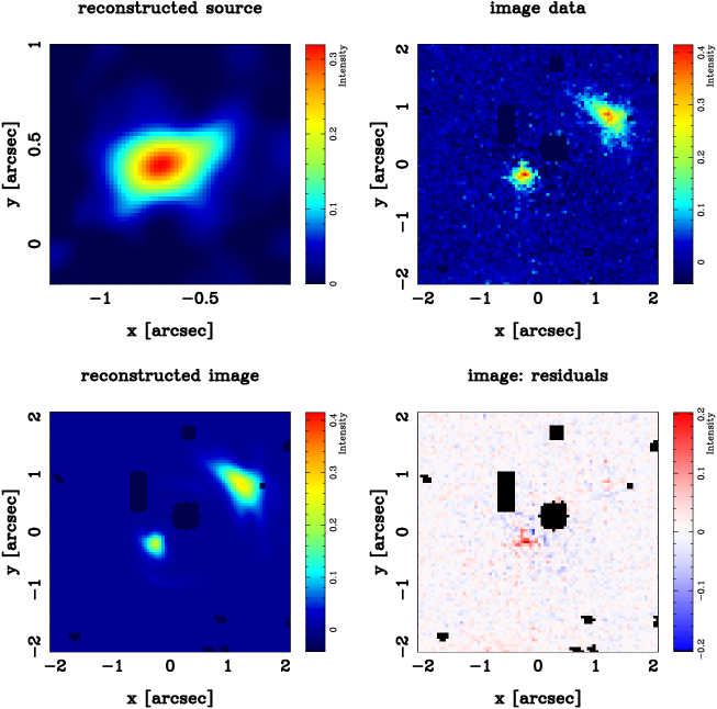
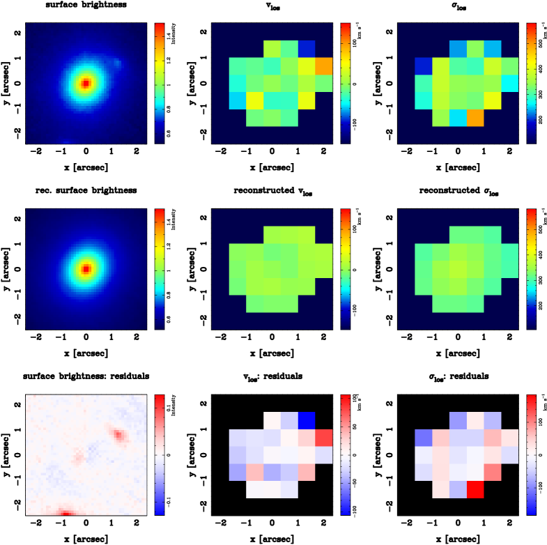
Figure 12: Best model lens image reconstruction for the system SDSS J0935. From the top left-hand to bottom right-hand panel: reconstructed source model; HST/ACS data showing the lens image after subtraction of the lens galaxy; lens image reconstruction; residuals. In the panels, North is up and East is to the right.

Figure 13: Best dynamical model for the galaxy SDSS J0935. First row: observed surface brightness distribution, projected line-of-sight velocity and line-of-sight velocity dispersion. Second row: corresponding reconstructed quantities for the best model. Third row: residuals. In the panels, North is up and East is to the right.

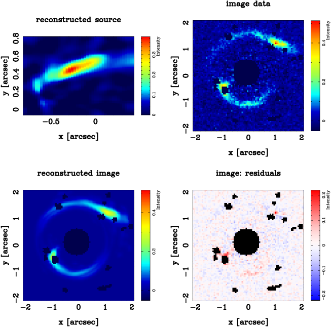
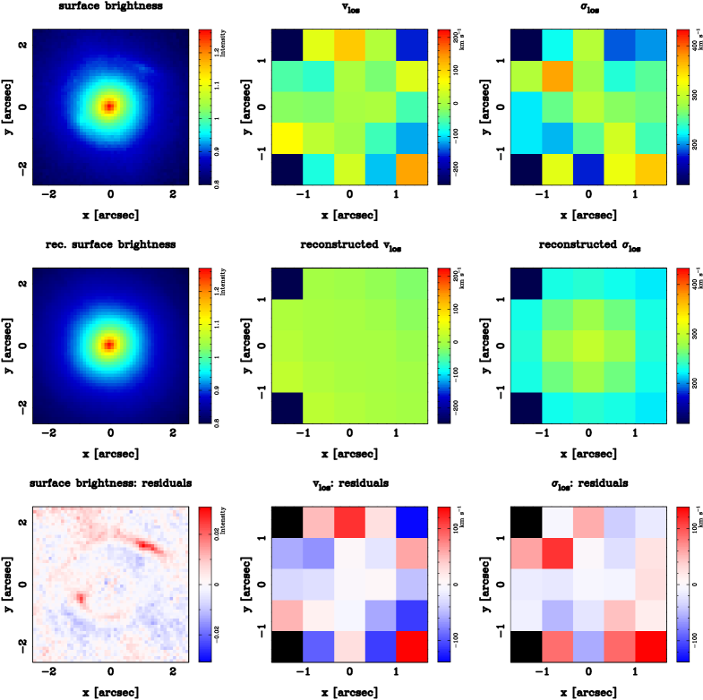
Figure 14: Best model lens image reconstruction for the galaxy SDSS J1204. Panels meaning as in Fig. 13.

Figure 15: Best dynamical model for the galaxy SDSS J1204. Panels meaning as in Fig. 13.

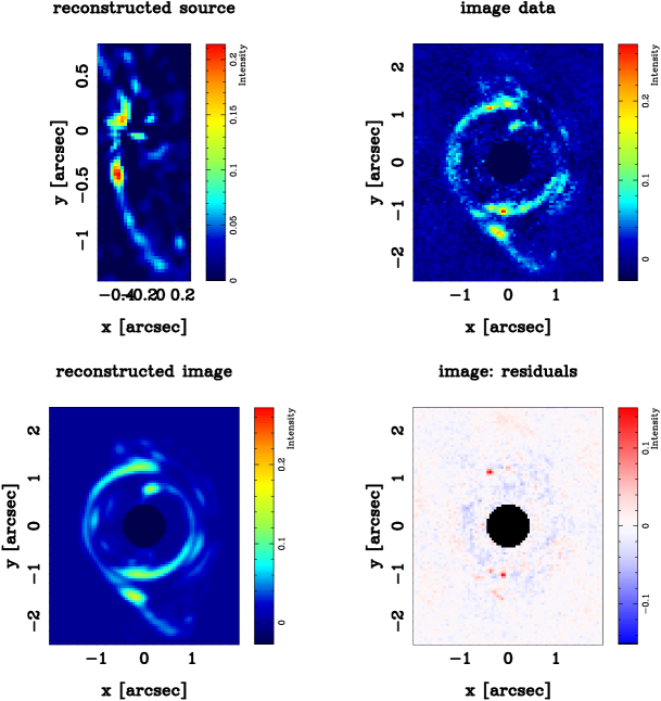
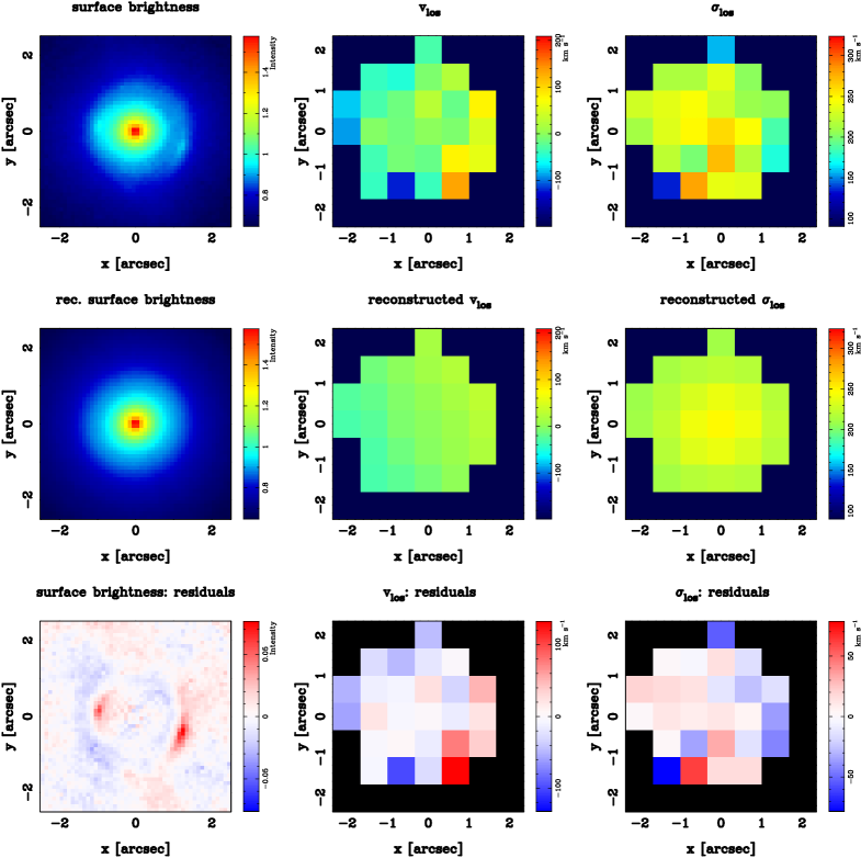
Figure 16: Best model lens image reconstruction for the galaxy SDSS J1250. Panels meaning as in Fig. 13.

Figure 17: Best dynamical model for the galaxy SDSS J1250. Panels meaning as in Fig. 13.

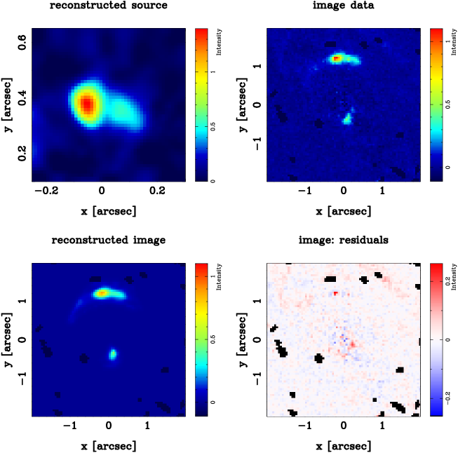
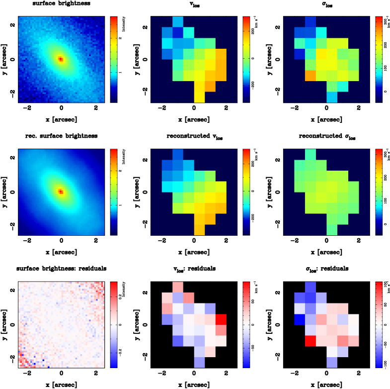
Figure 18: Best model lens image reconstruction for the galaxy SDSS J1251. Panels meaning as in Fig. 13.

Figure 19: Best dynamical model for the galaxy SDSS J1251. Panels meaning as in Fig. 13.

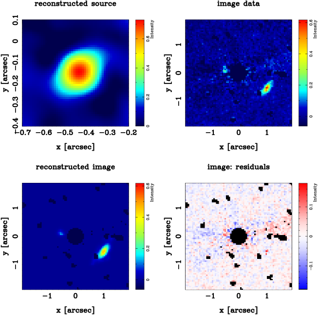
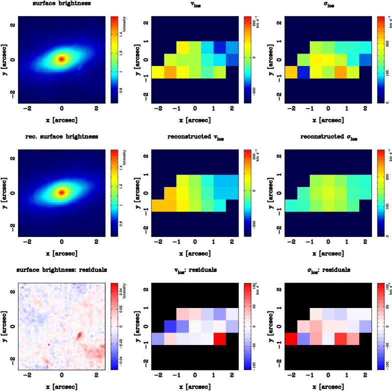
Figure 20: Best model lens image reconstruction for the galaxy SDSS J1330. Panels meaning as in Fig. 13.

Figure 21: Best dynamical model for the galaxy SDSS J1330. Panels meaning as in Fig. 13.

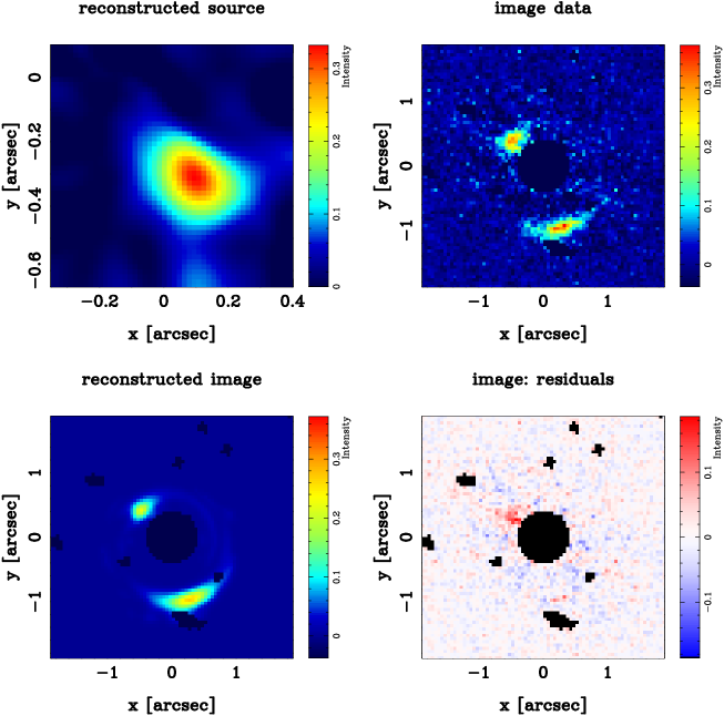
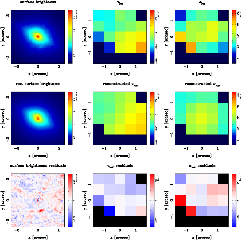
Figure 22: Best model lens image reconstruction for the galaxy SDSS J1443. Panels meaning as in Fig. 13.

Figure 23: Best dynamical model for the galaxy SDSS J1443. Panels meaning as in Fig. 13.

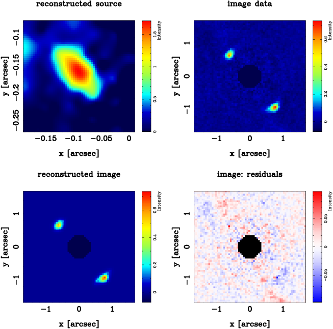
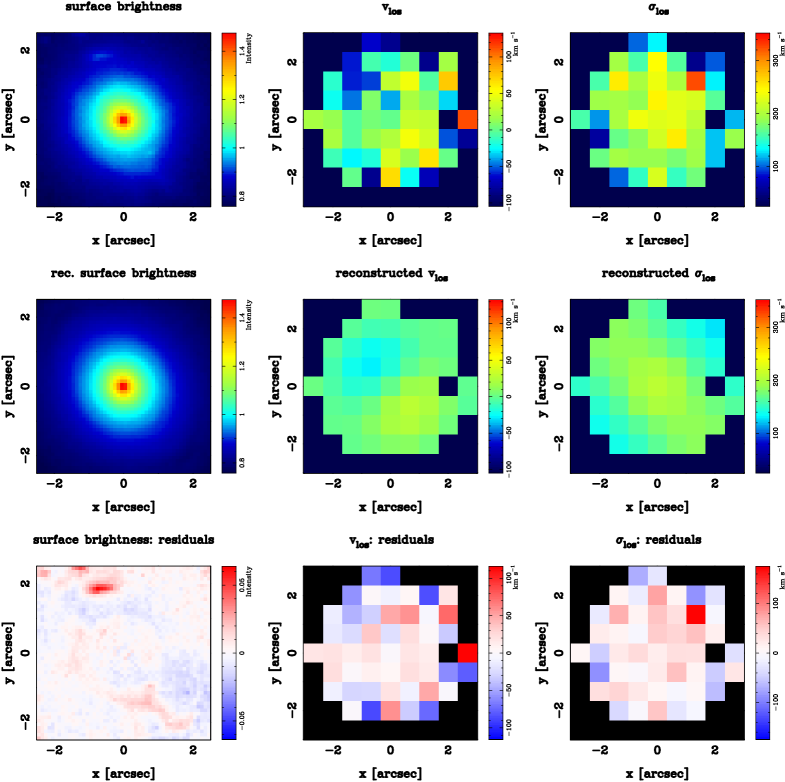
Figure 24: Best model lens image reconstruction for the galaxy SDSS J1451. Panels meaning as in Fig. 13.

Figure 25: Best dynamical model for the galaxy SDSS J1451. Panels meaning as in Fig. 13.

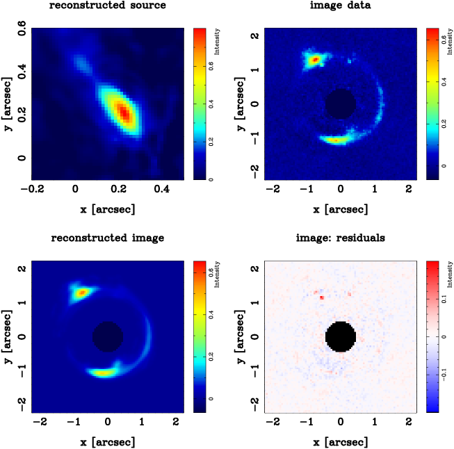
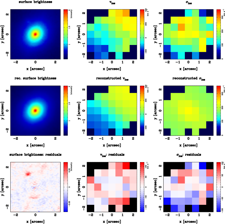
Figure 26: Best model lens image reconstruction for the galaxy SDSS J2238. Panels meaning as in Fig. 13.

Figure 27: Best dynamical model for the galaxy SDSS J2238. Panels meaning as in Fig. 13.

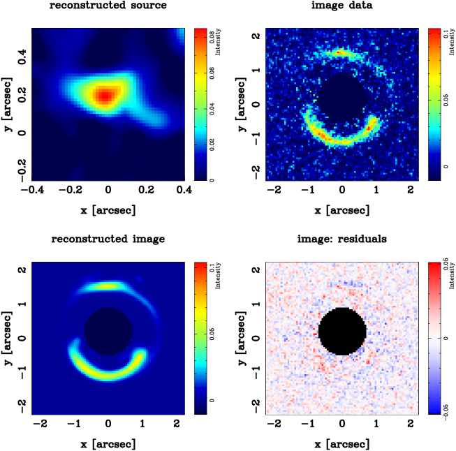
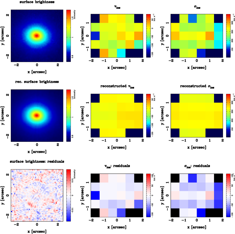
Figure 28: Best model lens image reconstruction for the galaxy SDSS J2300. Panels meaning as in Fig. 13.

Figure 29: Best dynamical model for the galaxy SDSS J2300. Panels meaning as in Fig. 13.

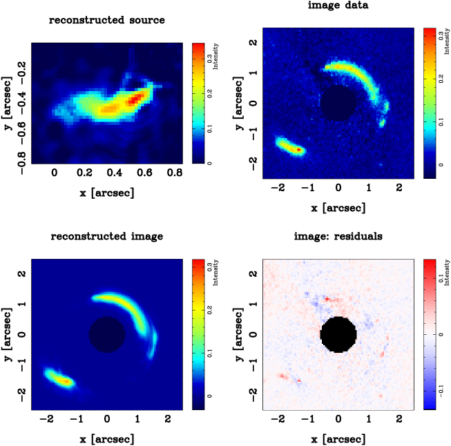
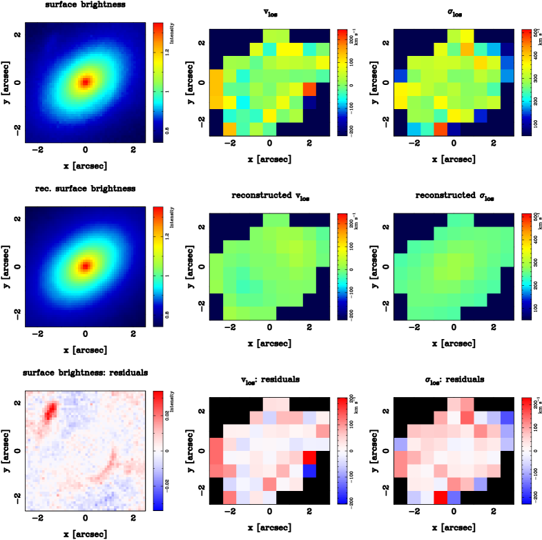
Figure 30: Best model lens image reconstruction for the galaxy SDSS J2303. Panels meaning as in Fig. 13.

Figure 31: Best dynamical model for the galaxy SDSS J2303. Panels meaning as in Fig. 13.

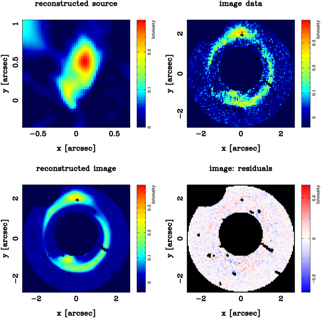
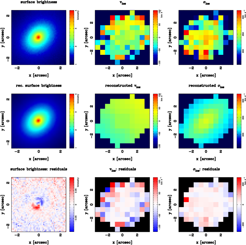
Figure 32: Best model lens image reconstruction for the galaxy SDSS J2321. Panels meaning as in Fig. 13.

Figure 33: Best dynamical model for the galaxy SDSS J2321. Panels meaning as in Fig. 13.

Appendix B Uncertainties

In this Appendix we present, for all the analyzed systems, the one-dimensional marginalized posterior PDFs for the considered model parameters ($i$, $\gamma^{\prime}$, $\alpha_{0}$, $q$), from which the corresponding uncertainties (quoted in the Table 1) are derived.

(a) J0037

(b) J0216

 

(c) J0912

(d) J0935

 

(e) J0959

(f) J1204

 

(g) J1250

(h) J1251

 

(i) J1330

(j) J1443

 

(k) J1451

(l) J1627

 

(m) J2238

(n) J2300

 

(o) J2303

(p) J2321

 

Figure 34: Marginalized posterior probability distribution functions of the power-law model parameters $i$ (inclination), $\gamma^{\prime}$ (logarithmic slope), $\alpha_{0}$ (lens strength) and $q$ (axial ratio) for each of the analyzed systems, obtained from the nested sampling evidence exploration (see text, Sect. 3.3). From left to right, top to bottom, the galaxy are presented in the same order as in Tables 1 and 2.

References

- Abadi et al. (2010) Abadi, M. G., Navarro, J. F., Fardal, M., Babul, A., & Steinmetz, M. 2010, MNRAS, 407, 435
- Auger et al. (2009) Auger, M. W., Treu, T., Bolton, A. S., Gavazzi, R., Koopmans, L. V. E., Marshall, P. J., Bundy, K., & Moustakas, L. A. 2009, ApJ, 705, 1099
- Auger et al. (2010a) Auger, M. W., Treu, T., Bolton, A. S., Gavazzi, R., Koopmans, L. V. E., Marshall, P. J., Moustakas, L. A., & Burles, S. 2010a, ApJ, 724, 511
- Auger et al. (2010b) Auger, M. W., Treu, T., Gavazzi, R., Bolton, A. S., Koopmans, L. V. E., & Marshall, P. J. 2010b, ApJ, 721, L163
- Barnabè et al. (2010) Barnabè, M., Auger, M. W., Treu, T., Koopmans, L. V. E., Bolton, A. S., Czoske, O., & Gavazzi, R. 2010, MNRAS, 406, 2339
- Barnabè et al. (2009a) Barnabè, M., Czoske, O., Koopmans, L. V. E., Treu, T., Bolton, A. S., & Gavazzi, R. 2009a, MNRAS, 399, 21
- Barnabè & Koopmans (2007) Barnabè, M., & Koopmans, L. V. E. 2007, ApJ, 666, 726
- Barnabè et al. (2009b) Barnabè, M., Nipoti, C., Koopmans, L. V. E., Vegetti, S., & Ciotti, L. 2009b, MNRAS, 393, 1114
- Bertin et al. (1994) Bertin, G. et al. 1994, A&A, 292, 381
- Binney (2005) Binney, J. 2005, MNRAS, 363, 937
- Binney & Tremaine (2008) Binney, J., & Tremaine, S. 2008, Galactic Dynamics: Second Edition (Princeton University Press)
- Bolton et al. (2008a) Bolton, A. S., Burles, S., Koopmans, L. V. E., Treu, T., Gavazzi, R., Moustakas, L. A., Wayth, R., & Schlegel, D. J. 2008a, ApJ, 682, 964
- Bolton et al. (2005) Bolton, A. S., Burles, S., Koopmans, L. V. E., Treu, T., & Moustakas, L. A. 2005, ApJ, 624, L21
- Bolton et al. (2006) —. 2006, ApJ, 638, 703
- Bolton et al. (2008b) Bolton, A. S., Treu, T., Koopmans, L. V. E., Gavazzi, R., Moustakas, L. A., Burles, S., Schlegel, D. J., & Wayth, R. 2008b, ApJ, 684, 248
- Borriello et al. (2003) Borriello, A., Salucci, P., & Danese, L. 2003, MNRAS, 341, 1109
- Cappellari et al. (2006) Cappellari, M. et al. 2006, MNRAS, 366, 1126
- Cappellari et al. (2007) —. 2007, MNRAS, 379, 418
- Cappellari et al. (2010) —. 2010, MNRAS, in press
- Carollo et al. (1995) Carollo, C. M., de Zeeuw, P. T., van der Marel, R. P., Danziger, I. J., & Qian, E. E. 1995, ApJ, 441, L25
- Chabrier (2003) Chabrier, G. 2003, PASP, 115, 763
- Chandrasekhar (1969) Chandrasekhar, S. 1969, Ellipsoidal Figures of Equilibrium (Yale University Press)
- Churazov et al. (2010) Churazov, E. et al. 2010, MNRAS, 404, 1165
- Coccato et al. (2009) Coccato, L. et al. 2009, MNRAS, 394, 1249
- Cole et al. (2000) Cole, S., Lacey, C. G., Baugh, C. M., & Frenk, C. S. 2000, MNRAS, 319, 168
- Côté et al. (2003) Côté, P., McLaughlin, D. E., Cohen, J. G., & Blakeslee, J. P. 2003, ApJ, 591, 850
- Cretton et al. (1999) Cretton, N., de Zeeuw, P. T., van der Marel, R. P., & Rix, H.-W. 1999, ApJS, 124, 383
- Czoske et al. (2008) Czoske, O., Barnabè, M., Koopmans, L. V. E., Treu, T., & Bolton, A. S. 2008, MNRAS, 384, 987
- Das et al. (2010) Das, P., Gerhard, O., Churazov, E., & Zhuravleva, I. 2010, MNRAS, 409, 1362
- de Lorenzi et al. (2009) de Lorenzi, F. et al. 2009, MNRAS, 395, 76
- de Zeeuw et al. (2002) de Zeeuw, P. T. et al. 2002, MNRAS, 329, 513
- Debattista et al. (2008) Debattista, V. P., Moore, B., Quinn, T., Kazantzidis, S., Maas, R., Mayer, L., Read, J., & Stadel, J. 2008, ApJ, 681, 1076
- Dehnen (2005) Dehnen, W. 2005, MNRAS, 360, 892
- Dutton et al. (2011) Dutton, A. A. et al. 2011, arXiv:astro-ph/1101.1622
- Dutton et al. (2010) Dutton, A. A., Conroy, C., van den Bosch, F. C., Prada, F., & More, S. 2010, MNRAS, 407, 2
- Dye et al. (2008) Dye, S., Evans, N. W., Belokurov, V., Warren, S. J., & Hewett, P. 2008, MNRAS, 388, 384
- Elmegreen et al. (2009) Elmegreen, D. M., Elmegreen, B. G., Marcus, M. T., Shahinyan, K., Yau, A., & Petersen, M. 2009, ApJ, 701, 306
- Emsellem et al. (2007) Emsellem, E. et al. 2007, MNRAS, 379, 401
- Feroz & Hobson (2008) Feroz, F., & Hobson, M. P. 2008, MNRAS, 384, 449
- Feroz et al. (2009) Feroz, F., Hobson, M. P., & Bridges, M. 2009, MNRAS, 398, 1601
- Franx et al. (1994) Franx, M., van Gorkom, J. H., & de Zeeuw, T. 1994, ApJ, 436, 642
- Fukazawa et al. (2006) Fukazawa, Y., Botoya-Nonesa, J. G., Pu, J., Ohto, A., & Kawano, N. 2006, ApJ, 636, 698
- Fukugita et al. (1998) Fukugita, M., Hogan, C. J., & Peebles, P. J. E. 1998, ApJ, 503, 518
- Gavazzi et al. (2008) Gavazzi, R., Treu, T., Koopmans, L. V. E., Bolton, A. S., Moustakas, L. A., Burles, S., & Marshall, P. J. 2008, ApJ, 677, 1046
- Gavazzi et al. (2007) Gavazzi, R., Treu, T., Rhodes, J. D., Koopmans, L. V. E., Bolton, A. S., Burles, S., Massey, R. J., & Moustakas, L. A. 2007, ApJ, 667, 176
- Gerhard et al. (2001) Gerhard, O., Kronawitter, A., Saglia, R. P., & Bender, R. 2001, AJ, 121, 1936
- Gerhard (1993) Gerhard, O. E. 1993, MNRAS, 265, 213
- Gnedin et al. (2004) Gnedin, O. Y., Kravtsov, A. V., Klypin, A. A., & Nagai, D. 2004, ApJ, 616, 16
- González-García et al. (2009) González-García, A. C., Oñorbe, J., Domínguez-Tenreiro, R., & Gómez-Flechoso, M. Á. 2009, A&A, 497, 35
- Graham et al. (2006) Graham, A. W., Merritt, D., Moore, B., Diemand, J., & Terzić, B. 2006, AJ, 132, 2701
- Graves & Faber (2010) Graves, G. J., & Faber, S. M. 2010, ApJ, 717, 803
- Grillo (2010) Grillo, C. 2010, ApJ, 722, 779
- Grillo et al. (2008) Grillo, C., Gobat, R., Rosati, P., & Lombardi, M. 2008, A&A, 477, L25
- Humphrey & Buote (2010) Humphrey, P. J., & Buote, D. A. 2010, MNRAS, 403, 2143
- Jesseit et al. (2007) Jesseit, R., Naab, T., Peletier, R. F., & Burkert, A. 2007, MNRAS, 376, 997
- Jiang & Kochanek (2007) Jiang, G., & Kochanek, C. S. 2007, ApJ, 671, 1568
- Johansson et al. (2009) Johansson, P. H., Naab, T., & Ostriker, J. P. 2009, ApJ, 697, L38
- Kazantzidis et al. (2006) Kazantzidis, S., Zentner, A. R., & Kravtsov, A. V. 2006, ApJ, 641, 647
- Koopmans (2005) Koopmans, L. V. E. 2005, MNRAS, 363, 1136
- Koopmans et al. (2009) Koopmans, L. V. E. et al. 2009, ApJ, 703, L51
- Koopmans & Treu (2003) Koopmans, L. V. E., & Treu, T. 2003, ApJ, 583, 606
- Koopmans et al. (2006) Koopmans, L. V. E., Treu, T., Bolton, A. S., Burles, S., & Moustakas, L. A. 2006, ApJ, 649, 599
- Kronawitter et al. (2000) Kronawitter, A., Saglia, R. P., Gerhard, O., & Bender, R. 2000, A&AS, 144, 53
- Kroupa (2001) Kroupa, P. 2001, MNRAS, 322, 231
- Lackner & Ostriker (2010) Lackner, C. N., & Ostriker, J. P. 2010, ApJ, 712, 88
- Loewenstein & White (1999) Loewenstein, M., & White, R. E. 1999, ApJ, 518, 50
- MacKay (1999) MacKay, D. J. C. 1999, Neural Comp, 11, 1035
- MacKay (2003) —. 2003, Information Theory, Inference and Learning Algorithms (Cambridge University Press)
- Mamon & Łokas (2005) Mamon, G. A., & Łokas, E. L. 2005, MNRAS, 362, 95
- Matsushita et al. (1998) Matsushita, K., Makishima, K., Ikebe, Y., Rokutanda, E., Yamasaki, N., & Ohashi, T. 1998, ApJ, 499, L13
- Meza et al. (2003) Meza, A., Navarro, J. F., Steinmetz, M., & Eke, V. R. 2003, ApJ, 590, 619
- Naab et al. (2007) Naab, T., Johansson, P. H., Ostriker, J. P., & Efstathiou, G. 2007, ApJ, 658, 710
- Napolitano et al. (2009) Napolitano, N. R. et al. 2009, MNRAS, 393, 329
- Napolitano et al. (2010) Napolitano, N. R., Romanowsky, A. J., & Tortora, C. 2010, MNRAS, 405, 2351
- Navarro et al. (1996) Navarro, J. F., Frenk, C. S., & White, S. D. M. 1996, ApJ, 462, 563
- Navarro et al. (2010) Navarro, J. F. et al. 2010, MNRAS, 402, 21
- Nipoti et al. (2009) Nipoti, C., Treu, T., & Bolton, A. S. 2009, ApJ, 703, 1531
- Oñorbe et al. (2007) Oñorbe, J., Domínguez-Tenreiro, R., Sáiz, A., & Serna, A. 2007, MNRAS, 376, 39
- Oosterloo et al. (2002) Oosterloo, T. A., Morganti, R., Sadler, E. M., Vergani, D., & Caldwell, N. 2002, AJ, 123, 729
- Padmanabhan et al. (2004) Padmanabhan, N. et al. 2004, New Astronomy, 9, 329
- Press et al. (1992) Press, W. H., Teukolsky, S. A., Vetterling, W. T., & Flannery, B. P. 1992, Numerical recipes in FORTRAN. The art of scientific computing (Cambridge: University Press, 2nd ed.)
- Renzini (2006) Renzini, A. 2006, ARAA, 44, 141
- Rix et al. (1997) Rix, H.-W., de Zeeuw, P. T., Cretton, N., van der Marel, R. P., & Carollo, C. M. 1997, ApJ, 488, 702
- Rodionov & Athanassoula (2011) Rodionov, S. A., & Athanassoula, E. 2011, MNRAS, 410, 111
- Romanowsky et al. (2003) Romanowsky, A. J., Douglas, N. G., Arnaboldi, M., Kuijken, K., Merrifield, M. R., Napolitano, N. R., Capaccioli, M., & Freeman, K. C. 2003, Science, 301, 1696
- Romanowsky et al. (2009) Romanowsky, A. J., Strader, J., Spitler, L. R., Johnson, R., Brodie, J. P., Forbes, D. A., & Ponman, T. 2009, AJ, 137, 4956
- Ruff et al. (2011) Ruff, A. J., Gavazzi, R., Marshall, P. J., Treu, T., Auger, M. W., & Brault, F. 2011, ApJ, 727, 96
- Rusin & Kochanek (2005) Rusin, D., & Kochanek, C. S. 2005, ApJ, 623, 666
- Saglia et al. (1992) Saglia, R. P., Bertin, G., & Stiavelli, M. 1992, ApJ, 384, 433
- Salpeter (1955) Salpeter, E. E. 1955, ApJ, 121, 161
- Schneider et al. (2006) Schneider, P., Kochanek, C. S., & Wambsganss, J. 2006, Gravitational Lensing: Strong, Weak and Micro, Saas-Fee Advanced Courses, 33 (Berlin, Springer-Verlag)
- Schwarzschild (1979) Schwarzschild, M. 1979, ApJ, 232, 236
- Sivia & Skilling (2006) Sivia, D. S., & Skilling, J. 2006, Data Analysis: A Bayesian Tutorial (Oxford University Press)
- Skilling (2004) Skilling, J. 2004, in American Institute of Physics Conference Series, Vol. 735, American Institute of Physics Conference Series, ed. R. Fischer, R. Preuss, & U. V. Toussaint, 395–405
- Spiniello et al. (2011) Spiniello, C., Koopmans, L. V. E., Trager, S. C., Czoske, O., & Treu, T. 2011, arXiv:astro-ph/1103.4773
- Suyu et al. (2006) Suyu, S. H., Marshall, P. J., Hobson, M. P., & Blandford, R. D. 2006, MNRAS, 371, 983
- Thomas (2010) Thomas, J. 2010, Reviews in Modern Astronomy, 22, 143
- Thomas et al. (2007) Thomas, J., Saglia, R. P., Bender, R., Thomas, D., Gebhardt, K., Magorrian, J., Corsini, E. M., & Wegner, G. 2007, MNRAS, 382, 657
- Thomas et al. (2009) —. 2009, ApJ, 691, 770
- Thomas et al. (2011) Thomas, J. et al. 2011, MNRAS, in press
- Tissera et al. (2010) Tissera, P. B., White, S. D. M., Pedrosa, S., & Scannapieco, C. 2010, MNRAS, 406, 922
- Toomre (1977) Toomre, A. 1977, in Evolution of Galaxies and Stellar Populations, ed. B. M. Tinsley & R. B. Larson, 401
- Tortora et al. (2009) Tortora, C., Napolitano, N. R., Romanowsky, A. J., Capaccioli, M., & Covone, G. 2009, MNRAS, 396, 1132
- Treu et al. (2010) Treu, T., Auger, M. W., Koopmans, L. V. E., Gavazzi, R., Marshall, P. J., & Bolton, A. S. 2010, ApJ, 709, 1195
- Treu et al. (2009) Treu, T., Gavazzi, R., Gorecki, A., Marshall, P. J., Koopmans, L. V. E., Bolton, A. S., Moustakas, L. A., & Burles, S. 2009, ApJ, 690, 670
- Treu & Koopmans (2002) Treu, T., & Koopmans, L. V. E. 2002, ApJ, 575, 87
- Treu & Koopmans (2004) —. 2004, ApJ, 611, 739
- Treu et al. (2006) Treu, T., Koopmans, L. V. E., Bolton, A. S., Burles, S., & Moustakas, L. 2006, ApJ, 640, 662
- Treu et al. (2002) Treu, T., Stiavelli, M., Casertano, S., Møller, P., & Bertin, G. 2002, ApJ, 564, L13
- Trott et al. (2010) Trott, C. M., Treu, T., Koopmans, L. V. E., & Webster, R. L. 2010, MNRAS, 401, 1540
- Trujillo et al. (2004) Trujillo, I., Burkert, A., & Bell, E. F. 2004, ApJ, 600, L39
- Tu et al. (2009) Tu, H. et al. 2009, A&A, 501, 475
- van Albada & Sancisi (1986) van Albada, T. S., & Sancisi, R. 1986, Royal Society of London Philosophical Transactions Series A, 320, 447
- van de Ven et al. (2010) van de Ven, G., Falcón-Barroso, J., McDermid, R. M., Cappellari, M., Miller, B. W., & de Zeeuw, P. T. 2010, ApJ, 719, 1481
- van den Bosch et al. (2008) van den Bosch, R. C. E., van de Ven, G., Verolme, E. K., Cappellari, M., & de Zeeuw, P. T. 2008, MNRAS, 385, 647
- van der Marel & Franx (1993) van der Marel, R. P., & Franx, M. 1993, ApJ, 407, 525
- van Dokkum & Conroy (2010) van Dokkum, P. G., & Conroy, C. 2010, Nature, 468, 940
- Verolme & de Zeeuw (2002) Verolme, E. K., & de Zeeuw, P. T. 2002, MNRAS, 331, 959
- Warren & Dye (2003) Warren, S. J., & Dye, S. 2003, ApJ, 590, 673
- Weijmans (2009) Weijmans, A.-M. 2009, PhD thesis, Leiden University
- Weijmans et al. (2009) Weijmans, A.-M. et al. 2009, MNRAS, 398, 561
- Weijmans et al. (2008) Weijmans, A.-M., Krajnović, D., van de Ven, G., Oosterloo, T. A., Morganti, R., & de Zeeuw, P. T. 2008, MNRAS, 383, 1343
- White & Frenk (1991) White, S. D. M., & Frenk, C. S. 1991, ApJ, 379, 52
- Zamojski et al. (2007) Zamojski, M. A. et al. 2007, ApJS, 172, 468