Fast iteration of cocyles over rotations and Computation of hyperbolic bundles

Abstract.

In this paper, we develop numerical algorithms that use small requirements of storage and operations for the computation of hyperbolic cocycles over a rotation. We present fast algorithms for the iteration of the quasi-periodic cocycles and the computation of the invariant bundles, which is a preliminary step for the computation of invariant whiskered tori.

1. Introduction

The goal of this paper is to describe efficient algorithms to compute quasi-periodic cocycles over rotations. We present fast algorithms for the iteration of cocycles over rotations and for the calculation of their invariant bundles. The main idea is to use a renormalization algorithm which allows to pass from a cocycle to a longer cocycle.

The calculation of invariant bundles for cocycles is a preliminary step for the calculation of whiskered invariant tori. Indeed, these algorithms require the computation of the projections over the linear subspaces of the linear cocycle.

2. Some standard definitions on cocycles

Given a matrix-valued function $M:{\mathbb{T}}^{\ell}\to GL(2d,{\mathbb{R}})$ and a vector $\omega\in{\mathbb{R}}^{\ell}$, we define the cocycle over the rotation $T_{\omega}$ associated to the matrix $M$ by a function ${\mathcal{M}}:{\mathbb{Z}}\times{\mathbb{T}}^{\ell}\to GL(2d,{\mathbb{R}})$ given by

$${\mathcal{M}}(n,\theta)=\begin{cases}M(\theta+(n-1)\omega)\cdots M(\theta)&n\geq 1,\\ \operatorname{Id}&n=0,\\ M^{-1}(\theta+(n+1)\omega)\cdots M^{-1}(\theta)&n\leq 1.\end{cases}$$ (2.1)

Equivalently, a cocycle is defined by the relation

$$\begin{split}{\mathcal{M}}(0,\theta)&=\operatorname{Id},\\ {\mathcal{M}}(1,\theta)&=M(\theta),\\ {\mathcal{M}}(n+m,\theta)&={\mathcal{M}}(n,T_{\omega}^{m}(\theta)){\mathcal{M}}(m,\theta).\end{split}$$ (2.2)

We will say that $M$ is the generator of ${\mathcal{M}}$. Note that if $M({\mathbb{T}}^{\ell})\subset G$ where $G\subset GL(2d,{\mathbb{R}})$ is a group, then ${\mathcal{M}}({\mathbb{Z}},{\mathbb{T}}^{\ell})\subset G$.

The main example of a cocycle in this paper is

$$M(\theta)=(DF\circ K)(\theta),$$

for $K$ a parameterization of an invariant torus satisfying the invariance equation

$$F\circ K=K\circ T_{\omega}.$$

Other examples appear in discrete Schrödinger equations [Pui02]. In the above mentioned examples, the cocycles lie in the symplectic group and in the unitary group, respectively.

Similarly, given a matrix valued function $M(\theta)$, a continuous in time cocycle ${\mathcal{M}}(t,\theta)$ is defined to be the unique solution of

$$\begin{split}\frac{d}{dt}{\mathcal{M}}(t,\theta)&=M(\theta+\omega t){\mathcal{M}}(t,\theta),\\ {\mathcal{M}}(0,\theta)&=\operatorname{Id}.\end{split}$$ (2.3)

From the uniqueness part of Cauchy-Lipschitz theorem, we have the following property

$$\begin{split}{\mathcal{M}}(\theta,t+s)&={\mathcal{M}}(\theta+\omega t,s){\mathcal{M}}(\theta,t),\\ {\mathcal{M}}(\theta,0)&=\operatorname{Id}.\end{split}$$ (2.4)

Note that (2.3) and (2.4) are the exact analogues of (2.1) and (2.2) in a continuous context. Moreover, if $M({\mathbb{T}}^{\ell})\subset{\mathfrak{G}}$, where ${\mathfrak{G}}$ is a sub-algebra of the Lie algebra of the Lie group $G$, then ${\mathcal{M}}({\mathbb{R}},{\mathbb{T}}^{\ell})\subset G$.

The main example for us of a continuous in time cocycle will be

$$M(\theta)=(DX\circ K)(\theta),$$

where $K$ is a solution of the invariance equation

$$\partial_{\omega}K=X\circ K$$

and $X$ is a Hamiltonian vector field. In this case, the cocycle ${\mathcal{M}}(\theta,t)$ is symplectic.

3. Hyperbolicity of cocycles

One of the most crucial property of cocycles is hyperbolicity (or spectral dichotomies) as described in [MS89, SS74, SS76a, SS76b, Sac78].

Definition 1.

Given $0<\lambda<\mu$ we say that a cocycle ${\mathcal{M}}(n,\theta)$ (resp. ${\mathcal{M}}(t,\theta)$) has a $\lambda,\mu-$ dichotomy if for every $\theta\in{\mathbb{T}}^{\ell}$ there exist a constant $c>0$ and a splitting depending on $\theta$,

$$T{\mathbb{R}}^{2d}={\mathcal{E}}^{s}\oplus{\mathcal{E}}^{u}$$

which is characterized by:

$$\begin{split}&(x_{\theta},v)\in{\mathcal{E}}^{s}\Leftrightarrow|{\mathcal{M}}(n,\theta)v|\leq c\lambda^{n}|v|\ ,\qquad\forall n\geq 0\\ &(x_{\theta},v)\in{\mathcal{E}}^{u}\Leftrightarrow|{\mathcal{M}}(n,\theta)v|\leq c\mu^{n}|v|\ ,\qquad\forall n\leq 0\end{split}$$ (3.1)

or, in the continuous time case

$$\begin{split}&(x_{\theta},v)\in{\mathcal{E}}^{s}\Leftrightarrow|{\mathcal{M}}(t,\theta)v|\leq c\lambda^{t}|v|\ ,\qquad\forall t\geq 0\\ &(x_{\theta},v)\in{\mathcal{E}}^{u}\Leftrightarrow|{\mathcal{M}}(t,\theta)v|\leq c\mu^{t}|v|\ ,\qquad\forall t\leq 0.\end{split}$$ (3.2)

The notation ${\mathcal{E}}^{s}$ and ${\mathcal{E}}^{u}$ is meant to suggest that an important case is the splitting between stable and unstable bundles. This is the case when $\lambda<1<\mu$ and the cocycle is said to be hyperbolic. Nevertheless, the theory developed in this section assumes only the existence of a spectral gap.

In the application to the computation of tori, $M(\theta)=(DF\circ K)(\theta)$ and $x_{\theta}=K(\theta)$. The existence of the spectral gap means that at every point of the invariant torus $K(\theta)$ one has a splitting so that the vectors grow with appropriate rates $\lambda,\mu$ under iteration of the cocycle. In the case of the invariant torus, it can be seen that the cocycle is just the fundamental matrix of the variational equations so that the cocycle describes the growth of infinitesimal perturbations.

It is well known that the mappings $\theta\to{\mathcal{E}}_{x_{\theta}}^{s,u}$ are $C^{r}$ if $M(.,)\in C^{r}$ for $r\in{\mathbb{N}}\cup\{\infty,\omega\}$ [HL06c]. This result uses heavily that the cocycles are over a rotation.

A system can have several dichotomies, but for the purposes of this paper, the definition 1 will be enough, since we can perform the analysis presented here for each gap.

One fundamental problem for subsequent applications is the computation of the invariant splittings (and, of course, to ensure their existence). The computation of the invariant bundles is closely related to the computation of iterations of the cocycle.

The first algorithm that comes to mind, is an analogue of the power method to compute leading eigenvalues of a matrix. Given a typical vector $(x_{\theta},v)\in{\mathcal{E}}^{u}$, we expect that, for $n\gg 1$, ${\mathcal{M}}(n,\theta)v$ will be a vector in ${\mathcal{E}}_{x_{T_{\omega}^{n}(\theta)}}^{u}$. Even if there are issues related to the $\theta$ dependence, this may be practical if ${\mathcal{E}}^{u}$ is a 1-dimensional bundle.

4. Equivalence of cocycles, reducibility

Reducibility is a very important issue in the theory of cocycles. We have the following definition.

Definition 2.

We say that a cocycle $\widetilde{M}(\theta)$ is equivalent to another cocycle $M(\theta)$ if there exists a matrix valued function $Q:{\mathbb{T}}^{\ell}\to GL(2d,{\mathbb{R}})$ such that

$$\widetilde{M}(\theta)=Q(\theta+\omega)^{-1}M(\theta)Q(\theta).$$ (4.1)

It is easy to check that $\widetilde{M}$ being equivalent to $M$ is an equivalence relation.

If $\widetilde{M}$ is equivalent to a constant cocycle (i.e. independent of $\theta$), we say that $\widetilde{M}$ is “reducible.”

The important point is that, when (4.1) holds, we have

$$\widetilde{{\mathcal{M}}}(n,\theta)=Q(\theta+n\omega)^{-1}{\mathcal{M}}(n,\theta)Q(\theta).$$ (4.2)

In particular, if $M$ is a constant matrix, we have

$$\widetilde{\mathcal{M}}(n,\theta)=Q^{-1}(\theta+n\omega)M^{n}Q(\theta),$$

so that the iterations of reducible cocycles are very easy to compute.

We will also see that one can alter the numerical stability properties of the iterations of cocycles by choosing appropriately $Q$. In that respect, it is also important to mention the concept of “quasi-reducibility” introduced by Eliasson [Eli01].

5. Algorithms for fast iteration of cocycles over rotations

In its simplest form, the algorithm for fast iteration of cocyles is:

Algorithm 1 (Iteration of cocycles $1$).

Given $M(\theta)$, compute

$$\widehat{M}(\theta)=M(\theta+\omega)M(\theta).$$ (5.1)

Set $\widehat{M}\to M$, $2\omega\to\omega$ and iterate the procedure.

We refer to $\widehat{M}$ as the renormalized cocycle and the procedure as a renormalization procedure.

The important property is that applying $k$ times the renormalization procedure described in Algorithm 1 amounts to compute the cocycle ${\mathcal{M}}(2^{k},\theta)$.

Then, if we discretize the matrix $M(\theta)$ taking $N$ points (or $N$ Fourier modes) and denote by $C(N)$ the number of operations required to perform a step of Algorithm 1, we can compute $2^{k}$ iterates at a cost of $kC(N)$ operations.

Notice that the important point is that the cost of computing $2^{k}$ iterations is proportional to $k$. Of course, the proportionality constant depends on $N$. The form of this dependence on $N$ depends on the details on how we compute the shift and the product of matrix valued functions.

There are several alternatives to perform the transformation (5.1). The main difficulty arises from the fact that, if we have points on a equally spaced grid, then $\theta+\omega$ will not be in the same grid. We have at least three alternatives:

1. Keep the discretization by points in a grid and compute $M(\theta+\omega)$ by interpolating with nearby points.

2. Keep the discretization by points in a grid but note that the shift is diagonal in Fourier space. Of course, the multiplication of the matrix is diagonal in real space.

3. Keep the discretization in Fourier space but use the Cauchy formula for the product.

The cost factor of each of these alternatives is, respectively,

$$\begin{split}&C_{1}(N)=O(N),\\ &C_{2}(N)=O(N\log N),\\ &C_{3}(N)=O(N^{2}).\end{split}$$ (5.2)

Besides their cost, the above algorithms may have different stability and roundoff properties. We are not aware of any study of these stability or round-off properties. The properties of interpolation depend on the dimension.

In each of the cases, the main idea of the method is to precompute some blocks of the iteration, store them and use them in future iteration. One can clearly choose different strategies to group the blocks. Possibly, different methods can lead to different numerical (in)stabilities. At this moment, we lack a definitive theory of stability which would allow us to choose the blocks.

Next, we will present an alternative consisting of using the $QR$ decomposition for the iterates. As described, for instance in [Ose68, ER85, DVV02], the $QR$ algorithm seems to be rather stable to compute iterates. One advantage is that, in the case of several gaps, it can compute all the eigenvalues in a stable way.

Algorithm 2 (Computation of cocycles with $QR$).

Given $M(\theta)$ and a $QR$ decomposition of $M(\theta)$,

$$M(\theta)=Q(\theta)R(\theta),$$

perform the following operations:

• Compute $S(\theta)=R(\theta+\omega)Q(\theta)$

• Compute pointwise a $QR$ decomposition of $S$, $S(\theta)=\bar{Q}(\theta)\bar{R}(\theta)$.

• Compute $\widetilde{Q}(\theta)=Q(\theta+\omega)\bar{Q}(\theta)$

• $\widetilde{R}(\theta)=\bar{R}(\theta)R(\theta+\omega)$

• $\widetilde{M}(\theta)=\widetilde{Q}(\theta)\widetilde{R}(\theta)$

• Set $M\leftarrow\widetilde{M}$

• $R\leftarrow\widetilde{R}$

• $Q\leftarrow\widetilde{Q}$

• $2\omega\leftarrow\omega$

and iterate the procedure.

Since the $QR$ decomposition is a fast algorithm, the total cost of the implementation depends on the issues previously discussed (see costs in (5.2)). Instead of using $QR$ decomposition, one can also perform a $SVD$ decomposition (which is somewhat slower).

In the case of one-dimensional maps, one can be more precise in the description of the method. Indeed, if the frequency $\omega$ has a continued fraction expansion

$$\omega=[a_{1},a_{2},\ldots,a_{n},\ldots],$$

it is well known that the denominators $q_{n}$ of the convergents of $\omega$ (i.e. $p_{n}/q_{n}=[a_{1},\ldots,a_{n}]$) satisfy

$$\begin{split}&q_{n}=a_{n}q_{n-1}+q_{n-2},\\ &q_{1}=a_{1},\\ &q_{0}=1.\end{split}$$

As a consequence, we can consider the following algorithm for this particular case:

Algorithm 3 (Iteration of cocycles $1D$).

Given $\omega=[a_{1},\ldots,a_{n},\ldots]$ and the cocycle over $T_{\omega}$ generated by $M(\theta)$, define

$$\omega^{0}=0,\qquad\omega^{1}=\omega,\qquad M^{0}(\theta)=\operatorname{Id},\qquad M^{1}(\theta)=M(\theta+(a_{1}-1)\omega)\cdots M(\theta).$$

Then, for $n\geq 2$

$$M^{(n)}(\theta)=M^{(n-1)}(\theta+(a_{n}-1)\omega^{n-1})\cdots M^{(n-1)}(\theta)M^{(n-2)}(\theta)$$

is a cocycle over

$$\omega^{n-1}=a_{n}\omega^{n-1}+\omega^{n-2}$$

and we have

$${\mathcal{M}}(q_{n},\theta)={\mathcal{M}}^{(n)}(1,\theta).$$

The advantage of this method is that the effective rotation is decreasing to zero so that the cocycle is becoming in some ways similar to the iteration of a constant matrix. This method is somehow reminiscent of some algorithms that have appeared in the mathematical literature [Ryc92, Kri99b, Kri99a].

6. The “straddle the saddle” phenomenon and preconditioning

The iteration of cocycles has several pitfalls compared with the iteration of matrices. The main complication from the numerical point of view is that the (un)stable bundle does depend on the base point.

In this section we describe a geometric phenomenon that causes some instability in the iteration of cocycles. This instability –which is genuine– becomes catastrophic when we apply some of the fast iteration methods described in Section 5. The phenomenon we will discuss was already observed in [HL06a].

Since we have the inductive relation,

$${\mathcal{M}}(n,\theta)={\mathcal{M}}(n-1,\theta+\omega)M(\theta),$$

we see that we can think of computing ${\mathcal{M}}(n,\theta)$ by applying ${\mathcal{M}}(n-1,\theta+\omega)$ to the column vectors of $M(\theta)$.

The $j^{th}$-column of $M$, which we will denote by $m_{j}(\theta)$, can be thought geometrically as an embedding from ${\mathbb{T}}^{\ell}$ to ${\mathbb{R}}^{2d}$ and is given by $M(\theta)e_{j}$ where $e_{j}$ is the $j^{th}$ vector of the canonical basis of ${\mathbb{R}}^{2d}$. If the stable space of ${\mathcal{M}}(n-1,\theta+\omega)$ has codimension $\ell$ or less, there could be points $\theta^{*}\in{\mathbb{T}}^{\ell}$ such that $m_{j}(\theta^{*})\in{\mathcal{E}}_{x_{\theta^{*}}}^{s}$ and such that for every $\theta\neq\theta^{*}$ we have $m_{j}(\theta)\notin{\mathcal{E}}_{x_{\theta}}^{s}$.

Clearly, the quantity

$${\mathcal{M}}(n-1,\theta^{*}+\omega)m_{j}(\theta^{*})$$

decreases exponentially. Nevertheless, for all $\theta$ in a neighborhood of $\theta^{*}$ such that $\theta\neq\theta^{*}$

$${\mathcal{M}}(n-1,\theta+\omega)m_{j}(\theta)$$

will grow exponentially. The direction along which the growth takes place depends on the projection of $m_{j}(\theta)$ on ${\mathcal{E}}_{x_{\theta+\omega}}^{u}$.

For example, in the case $d=2$, $\ell=1$ and the stable and unstable directions are one dimensional, the unstable components will have different signs and the vectors ${\mathcal{M}}(n-1,\theta+\omega)m_{j}(\theta)$ will align in opposite directions. An illustration of this phenomenon happens in Figure 1.

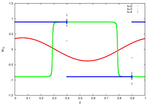
Figure 1. The straddle the saddle phenomenon. We plot one of the components of the cocycle ${\mathcal{M}}(2^{k},\theta)$ for the values $k=0,3,4$. The case $k=0$ was scaled by a factor $200$.

The transversal intersection of the range of $m_{j}(\theta)$ with ${\mathcal{E}}^{s}$ is indeed a true phenomenon, and it is a true instability.

Unfortunately, if $m_{j}(\theta)$ is very discontinuous as a function of $\theta$, the discretization in Fourier series or the interpolation by splines will be extremely inaccurate so that the Algorithm 1 fails to be relevant.

This phenomenon is easy to detect when it happens because the derivatives grow exponentially fast in some localized spots.

One important case where the straddle the saddle is unavoidable is when the invariant bundles are non-orientable. This happens near resonances (see [HL07]). In [HL07], it is shown that, by doubling the angle the case of resonances can be studied comfortably because then, non-orientability is the only obstruction to the triviality of the bundle.

6.1. Eliminating the “straddle the saddle” in the one-dimensional case

Fortunately, once the phenomenon is detected, it can be eliminated. The main idea is that one can find an equivalent cocycle which does not have the problem (or presents it in a smaller extent).

In more geometric terms we observe that, even if the stable and unstable bundles are geometrically natural objects, the decomposition of a matrix into columns is coordinate dependent. Hence, if we choose some coordinate system which is reasonably close to the stable and unstable manifolds and we denote by $Q$ the change of coordinates, then the cocycle

$$\widetilde{{\mathcal{M}}}(\theta)=Q(\theta+\omega)^{-1}M(\theta)Q(\theta),$$

is close to a constant. Remark that this is true only in the one-dimensional case. The picture is by far more involved when the bundles have higher rank.

This may seem somewhat circular, but the circularity can be broken using continuation methods. Given a cocycle which is close to constant, fast iteration methods work and they allow us to compute the splitting. Then if we have computed $Q$ for some $M$, we can use it to precondition the computation of neighboring $M$.

The algorithms for the computation of bundles will be discussed next.

6.2. Computation of rank-1 stable and unstable bundles using iteration of cocycles

The algorithms described in the previous section provide a fast way to iterate the cocycle. We will see that this iteration method, which is similar to the power method, gives the dominant eigenvalue $\lambda_{max}(\theta)$ and the corresponding eigenvector $m(\theta)$.

The methods based on iteration rely strongly on the fact that the cocycle has one dominating eigenvalue which is simple.

Consider that we have performed $k$ iterations of the cocycle (of course we perform scalings at each step) and we have computed ${\mathcal{M}}(n,\theta)$, with $n=2^{k}$. Then, one can easily read the dominant rank-1 bundle from the $QR$ decomposition of the cocycle ${\mathcal{M}}(n,\theta)$, just taking the column of $Q$ associated to the largest value in the diagonal of the upper triangular matrix $R$. One obtains a vector $m(\theta+2^{k}\omega)$ (and therefore $m(\theta)$ by performing a shift of angle $-2^{k}\omega$) of modulus 1 spanning the unstable manifold. Since,

$$M(\theta)m(\theta)=\lambda_{max}(\theta)m(\theta+\omega),$$

we have then

$$\lambda_{max}(\theta)=([M(\theta)m(\theta+\omega)]^{T}[M(\theta)m(\theta+\omega)])^{1/2}.$$

As it is standard in the power method, we perform scalings at each step dividing all the entries in the matrix $M(\theta)$ by the maximum value among the entries of the matrix.

Hence, for the simplest case that there is one dominant eigenvalue, the method produces a section $m$ (spanning the unstable subbundle) and a real function $\lambda_{max}$, which represents the dynamics on the rank 1 unstable subbundle, such that

$$M(\theta)m(\theta)=\lambda_{max}(\theta)m(\theta+\omega).$$

Following [HL06b], under certain non-resonant conditions which are satisfied in the case of the stable and unstable subspaces, one can reduce the 1-dimensional cocycle associated to $M$ and $\omega$ to a constant. Hence, we look for a positive function $p(\theta)$ and a constant $\mu$ such that

$$\lambda_{max}(\theta)p(\theta)=\mu p(\theta+\omega).$$ (6.1)

If $\lambda_{max}(\theta)>0$, we take logarithms on both sides of the equation (6.1). This leads to

$$\log\lambda_{max}(\theta)+\log p(\theta)=\log\mu+\log p(\theta+\omega),$$

and taking $\log\mu$ to be the average of $\log\lambda_{max}(\theta)$ the problem reduces to solve for $\log p(\theta)$. The case $\lambda_{max}(\theta)<0$ is analogous. Of course, $p(\theta)$ and $\mu$ can be obtained just exponentiating.

References

- [Ano69] D. V. Anosov. Geodesic flows on closed Riemann manifolds with negative curvature. American Mathematical Society, Providence, R.I., 1969.
- [Arn63] V. I. Arnol’d. Proof of a theorem of A. N. Kolmogorov on the invariance of quasi-periodic motions under small perturbations. Russian Math. Surveys, 18(5):9–36, 1963.
- [Arn64] V.I. Arnold. Instability of dynamical systems with several degrees of freedom. Sov. Math. Doklady, 5:581–585, 1964.
- [CFL03a] Xavier Cabré, Ernest Fontich, and Rafael de la Llave. The parameterization method for invariant manifolds. I. Manifolds associated to non-resonant subspaces. Indiana Univ. Math. J., 52(2):283–328, 2003.
- [CFL03b] Xavier Cabré, Ernest Fontich, and Rafael de la Llave. The parameterization method for invariant manifolds. II. Regularity with respect to parameters. Indiana Univ. Math. J., 52(2):329–360, 2003.
- [CL08] R. Calleja and R. de la Llave. Fast numerical computation of quasi-periodic equilibrium states in 1-d statistical mechanics, including twist maps. 2008. Manuscript.
- [DH08] Amadeu Delshams and Gemma Huguet. Geography of resonances and Arnold diffusion in a priori unstable Hamiltonian systems. Preprint, http://www.ma.utexas.edu/mp_arc, 08–227, 2008.
- [dlLR91] R. de la Llave and D. Rana. Accurate strategies for K.A.M. bounds and their implementation. In Computer Aided Proofs in Analysis (Cincinnati, OH, 1989), pages 127–146. Springer, New York, 1991.
- [DLS06] A. Delshams, R. de la Llave, and T. M. Seara. A geometric mechanism for diffusion in Hamiltonian systems overcoming the large gap problem: heuristics and rigorous verification on a model. Mem. Amer. Math. Soc., 179(844):viii+141, 2006.
- [DVV02] Luca Dieci and Erik S. Van Vleck. Lyapunov spectral intervals: theory and computation. SIAM J. Numer. Anal., 40(2):516–542 (electronic), 2002.
- [Eli01] L. H. Eliasson. Almost reducibility of linear quasi-periodic systems. In Smooth ergodic theory and its applications (Seattle, WA, 1999), volume 69 of Proc. Sympos. Pure Math., pages 679–705. Amer. Math. Soc., Providence, RI, 2001.
- [ER85] J.-P. Eckmann and D. Ruelle. Ergodic theory of chaos and strange attractors. Rev. Modern Phys., 57(3, part 1):617–656, 1985.
- [Fen72] Neil Fenichel. Persistence and smoothness of invariant manifolds for flows. Indiana Univ. Math. J., 21:193–226, 1971/1972.
- [Fen77] N. Fenichel. Asymptotic stability with rate conditions. II. Indiana Univ. Math. J., 26(1):81–93, 1977.
- [Fen74] N. Fenichel. Asymptotic stability with rate conditions. Indiana Univ. Math. J., 23:1109–1137, 1973/74.
- [FLS07] E. Fontich, R. de la Llave, and Y. Sire. Construction of invariant whiskered tori by a parametrization method. part I: Maps and flows in finite dimensions. Preprint, 2007.
- [GJSM01a] G. Gómez, À. Jorba, C. Simó, and J. Masdemont. Dynamics and mission design near libration points. Vol. III, volume 4 of World Scientific Monograph Series in Mathematics. World Scientific Publishing Co. Inc., River Edge, NJ, 2001. Advanced methods for collinear points.
- [GJSM01b] G. Gómez, À. Jorba, C. Simó, and J. Masdemont. Dynamics and mission design near libration points. Vol. IV, volume 5 of World Scientific Monograph Series in Mathematics. World Scientific Publishing Co. Inc., River Edge, NJ, 2001. Advanced methods for triangular points.
- [Gra74] Samuel M. Graff. On the conservation of hyperbolic invariant tori for Hamiltonian systems. J. Differential Equations, 15:1–69, 1974.
- [HL00] A. Haro and R. de la Llave. New mechanisms for lack of equipartion of energy. Phys. Rev. Lett., 89(7):1859–1862, 2000.
- [HL06a] À. Haro and R. de la Llave. Manifolds on the verge of a hyperbolicity breakdown. Chaos, 16(1):013120, 8, 2006.
- [HL06b] À. Haro and R. de la Llave. A parameterization method for the computation of invariant tori and their whiskers in quasi-periodic maps: numerical algorithms. Discrete Contin. Dyn. Syst. Ser. B, 6(6):1261–1300 (electronic), 2006.
- [HL06c] A. Haro and R. de la Llave. A parameterization method for the computation of invariant tori and their whiskers in quasi-periodic maps: rigorous results. J. Differential Equations, 228(2):530–579, 2006.
- [HL07] A. Haro and R. de la Llave. A parameterization method for the computation of whiskers in quasi periodic maps: numerical implementation and examples. SIAM Jour. Appl. Dyn. Syst., 6(1):142–207, 2007.
- [HPS77] M.W. Hirsch, C.C. Pugh, and M. Shub. Invariant manifolds, volume 583 of Lecture Notes in Math. Springer-Verlag, Berlin, 1977.
- [JO05] Àngel Jorba and Estrella Olmedo. A parallel method to compute quasi-periodic solutions. In EQUADIFF 2003, pages 181–183. World Sci. Publ., Hackensack, NJ, 2005.
- [JO08] Àngel Jorba and Estrella Olmedo. On the computation of reducible invariant tori in a parallel computer. Preprint, (08-2), 2008.
- [Kri99a] Raphaël Krikorian. -densité globale des systèmes produits-croisés sur le cercle réductibles. Ergodic Theory Dynam. Systems, 19(1):61–100, 1999.
- [Kri99b] Raphaël Krikorian. Réductibilité des systèmes produits-croisés à valeurs dans des groupes compacts. Astérisque, (259):vi+216, 1999.
- [LGJV05] R. de la Llave, A. González, À. Jorba, and J. Villanueva. KAM theory without action-angle variables. Nonlinearity, 18(2):855–895, 2005.
- [Lla01] Rafael de la Llave. A tutorial on KAM theory. In Smooth ergodic theory and its applications (Seattle, WA, 1999), pages 175–292. Amer. Math. Soc., Providence, RI, 2001.
- [LY05] Yong Li and Yingfei Yi. Persistence of hyperbolic tori in Hamiltonian systems. J. Differential Equations, 208(2):344–387, 2005.
- [MS89] Kenneth R. Meyer and George R. Sell. Mel′nikov transforms, Bernoulli bundles, and almost periodic perturbations. Trans. Amer. Math. Soc., 314(1):63–105, 1989.
- [Ose68] V. I. Oseledec. A multiplicative ergodic theorem. Characteristic Ljapunov, exponents of dynamical systems. Trudy Moskov. Mat. Obšč., 19:179–210, 1968.
- [Pes04] Yakov B. Pesin. Lectures on partial hyperbolicity and stable ergodicity. Zurich Lectures in Advanced Mathematics. European Mathematical Society (EMS), Zürich, 2004.
- [Pui02] J. Puig. Reducibility of linear differential equations with quasi-periodic coefficients: a survey. http://www.ma.utexas.edu/mp_arc, 02–246, 2002.
- [Ryc92] Marek Rychlik. Renormalization of cocycles and linear ODE with almost-periodic coefficients. Invent. Math., 110(1):173–206, 1992.
- [Sac78] R.J. Sacker. Existence of dichotomies and invariant splittings for linear differential systems. IV. J. Differential Equations, 27(1):106–137, 1978.
- [Sim99] Carles Simó, editor. Hamiltonian systems with three or more degrees of freedom, Dordrecht, 1999. Kluwer Academic Publishers Group.
- [Sim00] Carles Simó. private communication. 2000.
- [SS74] R.J. Sacker and G.R. Sell. Existence of dichotomies and invariant splittings for linear differential systems. I. J. Differential Equations, 15:429–458, 1974.
- [SS76a] R.J. Sacker and G.R. Sell. Existence of dichotomies and invariant splittings for linear differential systems. II. J. Differential Equations, 22(2):478–496, 1976.
- [SS76b] R.J. Sacker and G.R. Sell. Existence of dichotomies and invariant splittings for linear differential systems. III. J. Differential Equations, 22(2):497–522, 1976.
- [Zeh75] E. Zehnder. Generalized implicit function theorems with applications to some small divisor problems/I. Comm. Pure Appl. Math., 28:91–140, 1975.